Infill Well Placement Optimization for Polymer Flooding in Offshore Oil Reservoirs Using an Improved Archimedes Opti-Mization Algorithm with Halton Sequence

Preprint

Article

Infill Well Placement Optimization for Polymer Flooding in Offshore Oil Reservoirs Using an Improved Archimedes Opti-Mization Algorithm with Halton Sequence

Altmetrics

Downloads

Views

Comments

A peer-reviewed article of this preprint also exists.

Engao Tang,

Jian Zhang,Anlong Xia,Yi Jin,Lezhong Li,Jinju Chen,Biqin Hu,

Xiaofei Sun^*

Engao Tang,

Jian Zhang,Anlong Xia,Yi Jin,Lezhong Li,Jinju Chen,Biqin Hu,

Xiaofei Sun^*

This version is not peer-reviewed

Submitted:

20 August 2024

Posted:

22 August 2024

You are already at the latest version

Alerts

Abstract

Infill drilling is one of the most effective methods to improve the performance of poly-mer flooding. The difficulties related to infill drilling are determining the optimal numbers and placements of infill wells. In this study, an improved archimedes optimization algorithm with Halton sequence (HS-AOA) was proposed to overcome the aforementioned difficulties. First, to optimize the infill well placement for polymer flooding, an objective function that considered the economic influence of infill drilling was developed. Then, the novel optimization algorithm (HS-AOA) for infill well placement was developed by combining the AOA with the Halton se-quence. The codes were developed in MATLAB and connected to a commercial reservoir simula-tor CMG STARS to carry out the infill well placement optimization. Finally, the HS-AOA was compared to the basic AOA to confirm its reliability and then used to optimize the infill well placements for polymer flooding in a typical offshore oil reservoir. The results showed that the introduction of the Halton sequence into AOA effectively increased the diversity of the initial ob-jects in the AOA and avoided the HS-AOA trapping into the local optimal solutions. The HS–AOA outperformed the AOA. It was an effective approach to optimize the infill well placement for polymer flooding processes. In addition, infill drilling could effectively and economically im-prove the polymer flooding performance in offshore oil reservoirs. The NPV of the polymer flooding case with infill wells determined by HS-AOA reached 3.5 × 108 $, which was an increase of 7% over that of the polymer flooding case. This study presents an effective method for opti-mizing infill well placement for polymer flooding processes. It also can serve as a valuable refer-ence for other optimization problems in the petroleum industry, such as joint optimization of well control and placement.

Keywords:

Subject: Engineering - Other

1. Introduction

Polymer flooding is a low-risk, well-known, and commercial oil recovery method that uses polymers to increase the injected water viscosity thereby enhancing oil recovery [1,2,3]. The expected outcome of using polymer flooding is to achieve an additional 15% to 20% oil recovery compared to waterflooding [4]. Recently, as onshore oil resources start to reach peak production, offshore oil resources become increasingly attractive. Polymer flooding has been used in many offshore oil oilfields, such as the Dalia field (Angola), the Bohai oilfield (China), and the Dos Cuadras field (the United States) [5,6,7,8,9,10,11]. Infill drilling is one of the most effective methods to improve the performance of polymer flooding [12]. However, the difficulties related to infill drilling are determining optimal numbers and placements of infill wells. Therefore, infill well placement optimization is a crucial procedure for polymer flooding with infill wells in offshore oilfields.

Many factors, such as fluid properties, geological conditions, and development strategies affect optimal infill well placement. Therefore, the problem of infill well placement optimization is usually complex, nonlinear, and multimodal. To solve this problem, combining an optimization algorithm with a reservoir numerical simulator is a widely utilized approach [13,14,15,16]. The reservoir numerical simulator calculates the objective function (cumulative oil production or net present value (NPV)). The optimization algorithm is utilized to perform the optimization process. Therefore, determining a reliable optimization algorithm is important for infill well placement optimization [17,18,19].

There have been many previous studies addressing well placement optimization using various algorithms (particle swarm optimization (PSO) algorithm [20,21], genetic algorithm (GA) [22,23], and imperialist competitive algorithm (ICA) [16,24]). In particular, Emerick et al. (2009) used the GA to optimize the well number, well placement, and well trajectory in three-dimensional reservoir models [22]. Onwunalu and Durlofsky (2010) utilized the PSO algorithm to determine the optimal well placement and type (vertical and non-conventional wells) [25]. Al Dossary and Nasrabadi (2016) used ICA to find the optimal well placement by maximizing the cumulative oil production [26].

Recently, some hybrid optimization algorithms have been developed to improve the accuracy of well placement optimization. Hamida et al. (2017) proposed an improved GA for well placement optimization in which a similarity operator was added to the GA. They found that the modified GA had better performance than GA [27]. Khoshneshin and Sadeghnejad (2018) developed a modified PSO algorithm in which an inertia decrement was incorporated to affect the particle motion. They confirmed that the modified PSO algorithm had better performance than the basic PSO in determining the optimal well placements [28]. Janiga et al. (2019) utilized the self-adaptive clustering technique to decrease the search space of optimization algorithms. Their findings demonstrated that the execution time was reduced by 21% and 18% compared to GA and PSO, respectively [29].

In recent years, archimedes optimization algorithm (AOA) has gained significant attention as one of the promising metaheuristic algorithms. Its potential in various engineering applications was evaluated by many researchers. Hashim et al. (2021) used AOA to optimize the parameters of four problems in engineering design. They concluded that AOA was a highly effective approach in terms of convergence speed. It outperformed GA, PSO, and whale optimization algorithm (WOA) [30]. Abualigah et al. (2021) evaluated the performance of AOA on the design problems of a 3-bar truss, pressure vessel, and welded beam. The results showed that the AOA had better global optimization performance than eleven other optimization algorithms (Bat algorithm, differential evolution, grey wolf optimizer, etc.) [31]. Khan et al. (2022) validated that AOA was a promising optimization algorithm. It was particularly well-suited for solving the selective harmonic elimination problem and confirmed its superiority over GA [32].

The aforementioned studies demonstrated that AOA was used in many engineering applications and outperformed most well-known optimization algorithms. However, to the best of our knowledge, there has been no research on the application of AOA for infill well placement optimization problems. Therefore, in this study, AOA was introduced to determine the optimal infill well placement for polymer flooding in a typical offshore oil reservoir. However, AOA as a metaheuristic algorithm, also faces challenges like slow convergence speed or premature. To solve the problems, an improved AOA with Halton sequence (HS–AOA) was proposed in this study. First, to optimize the infill well placement for polymer flooding, an objective function that considered the economic influence of infill drilling was developed. Then, the novel optimization algorithm (HS-AOA) for infill well placement was developed by combining the AOA with the Halton sequence. The codes were developed in MATLAB and connected to a commercial reservoir simulator CMG STARS to carry out the infill well placement optimization. Finally, the HS-AOA was compared to the basic AOA to confirm its reliability and then used to optimize the infill well placements for polymer flooding in a typical offshore oil reservoir. This study presents an effective method for optimizing infill well placement for polymer flooding processes. It also can serve as a valuable reference for other optimization problems in the petroleum industry, such as joint optimization of well control and placement.

2. Methodology

2.1. Improved AOA with Halton Sequence

As described above, the AOA is superior to many metaheuristic algorithms. However, the AOA also faces many challenges. One of the important challenges is that the AOA easily traps into the local optimal solution because the initial objects are generated randomly in AOA, resulting in poor diversity. Therefore, the HS–AOA was proposed in this study to solve the aforementioned problem. Figure 1 presents the flowchart of HS–AOA, in which the initial objects are generated by the Halton sequence, followed by further optimization in the framework of the AOA.

The following are the detailed steps for developing the HS–AOA.

(1) Initialize the objects by Halton sequence

An arbitrary decimal integer t is converted into its corresponding numeral in base b: a₁(t), a₂(t), a₃(t), …, a_m(t), Subsequently, position the digits symmetrically to the right of the decimal point to obtain the number as illustrated in Equation (1):

Φ_{b} (t) = 0. a_{m} (t) a_{m - 1} (t) \dots a_{l} (t)

(1)

Where

Φ_{b} (t)

is the value of t in the Van der Corput sequence expressed in base b; m is the number of decimal places in

Φ_{b} (t)

; a_l(t) is the l^th digit of the b expansion of t in base b.

For distinct bases b and values of t are substituted into Equation (1), the Van der Corput sequences are generated. These sequences are then arranged to form a Halton sequence.

\vec{H a l t o n_{t}} = (Φ_{b_{1}} (t), Φ_{b_{2}} (t), \dots, Φ_{b_{n}} (t))

(2)

where

\vec{H a l t o n_{t}}

is the row of the Halton sequence，b₁、b₂…b_n represent n mutually prime integers starting from 1.

Initialize the volumes, accelerations, densities, and positions of all objects using Equation (3):

{\begin{cases} d_{i} (t) = r a n d \\ v_{i} (t) = r a n d \\ a_{i} (t) = l_{0} + r a n d \times (u_{0} - l_{0}) \\ \vec{x_{i} (t)} = \vec{l} + {\vec{H a l t o n}}_{t} \times (\vec{u} - \vec{l}) \end{cases} i = 1, 2, 3, \dots, N

(3)

Where v_i(t), a_i(t), d_i(t), and

\vec{x_{i} (t)}

are the volume, acceleration, density, and position of the object i at the t^th iteration, respectively;

\vec{x_{i} (t)}

includes the parameters that need to be optimized, such as the placements and numbers of infill wells; l₀ and

\vec{l}

are the lower limits of acceleration and position, respectively; u₀ and

\vec{u}

are the upper limits of acceleration and position, respectively.

(2) Calculate the object’s fitness

The parameters in the

\vec{x_{i} (t)}

of each object are input into an established reservoir simulation model for polymer flooding, and the oil production data are obtained by the simulation calculations. Then, the objective function (NPV) for drilling infill wells is calculated based on the economic parameters, such as the injection costs, drilling costs, and oil prices. The negative value of the NPV is treated as the fitness value as follows:

f i t n e s s_{i} (t) = - N P V_{i} (t), i = 1, 2, 3, \dots, N

(4)

where N is the total object number; fitness_i(t) and NPV_i(t) are the fitness value and the net present value of the object i at the t^th iteration, respectively.

(3) Update volumes and densities

Update the volume (v_i(t+1)) and density (d_i(t+1)) of the object i at the t+1^th iteration by using Equation (5):

{\begin{cases} v_{i} (t + 1) = r a n d \times (v_{b} (t) - v_{i} (t)) + v_{i} (t) \\ d_{i} (t + 1) = r a n d \times (d_{b} (t) - d_{i} (t)) + d_{i} (t) \end{cases}

(5)

where d_b(t) and v_b(t) are the object’s density and volume, respectively, which have the smallest fitness values at the t^th iteration.

The collisions between objects often result in the objects attempting to reach a state of equilibrium over time. The aforementioned process is described by Equation (6).

T O (t) = \exp (\frac{t - t_{\max}}{t_{\max}})

(6)

where TO(t) is the transfer operator; t_max is the maximum iteration number.

(4) Exploration phase

When the TO is equal to or less than 0.5, the collision does not occur between the objects. A random object is selected to update the acceleration as follows:

a_{i} (t + 1) = \frac{d_{m r} (t) + v_{m r} (t) \times a_{m r} (t)}{d_{i} (t + 1) \times v_{i} (t + 1)}

(7)

where a_i(t+1) is the acceleration of the object i at the t+1^th iteration; d_mr(t), a_mr(t), and v_mr(t) are a random object’s density, acceleration, and volume at the t^th iteration, respectively.

The

\vec{x_{i} (t + 1)}

is obtained as follows:

\vec{x_{i} (t + 1)} = a_{i - n} (t + 1) \times r a n d \times C_{1} \times D (t + 1) \times (\vec{x_{m r - r} (t)} - \vec{x_{i} (t)}) + \vec{x_{i} (t)}

(8)

where

\vec{x_{m r - r} (t)}

is the position of a random object at the t^th iteration; C₁ is a constant; D(t+1) is the density decreasing factor at the t+1^th iteration; a_i-n(t+1) is the normalized acceleration at the t+1^th iteration, which is calculated according to the following equation.

a_{i - n} (t + 1) = u_{a} \times \frac{a_{i} (t + 1) - \min (a_{i} (t + 1))}{\max (a_{i} (t + 1)) - \min (a_{i} (t + 1))} + l_{a}

(9)

where l_a and u_a are the lower and upper limits of a_i-n(t+1), respectively; The min(a_i(t+1)) and max(a_i(t+1)) are the minimum and maximum values of the object i’s acceleration at the t+1^th iteration, respectively.

The D(t+1) is calculated by using Equation (10):

D (t + 1) = \exp (1 - \frac{t}{t_{\max}}) - \frac{t}{t_{\max}}

(10)

When TO is greater than 0.5, the collision occurs between objects. The acceleration is updated with the optimal object.

a_{i} (t + 1) = \frac{d_{b} (t) + v_{b} (t) \times a_{b} (t)}{d_{i} (t + 1) \times v_{i} (t + 1)}

(11)

The

\vec{x_{i} (t + 1)}

is determined as follows:

\vec{x_{i} (t + 1)} = a_{i - n} (t + 1) \times D (t + 1) \times (C_{2} \times T O (t + 1) \times \vec{x_{b} (t)} - \vec{x_{i} (t)}) \times C_{3} \times F \times + \vec{x_{b} (t)}

(12)

where C₂ and C₃ are constants; TO(t+1) is the transfer operator at the t+1^th iteration; F is a flag to determine the motion direction, which is calculated by using Equation (13).

F = {\begin{cases} 1, \begin{matrix} 2 \times rand - C_{4} \leq 0.5 \end{matrix} \\ - 1 ， \begin{matrix} 2 \times rand - C_{4} \geq 0.5 \end{matrix} \end{cases}

(13)

where C₄ is a constant.

(5) Update fitness

After updating the object’s position, recalculate the fitness values of each object by using Step (2).

(6) Convergence

Repeat steps 2 to 5, and record the relationship between the fitness values and t. If all the objects have the same fitness value at the t^th iteration or t = t_max, the algorithm ends, and the

\vec{x_{b e s t} (t)}

is the best object’s position. The parameters in

\vec{x_{b e s t} (t)}

including the placements and numbers of infill wells are the optimal values.

2.2. Objective Function

In this study, the infill well placement was optimized to maximize the NPV. During the calculation of NPV, the economic influence of infill drilling should be considered. Taking the oil prices, polymer injection costs, and drilling costs into account, the NPV for polymer flooding with infill wells was calculated as follows:

N P V = \sum_{t = 0}^{T} \frac{C F_{t}}{{(1 + i)}^{t}}

(14)

C F_{t} = = （ Q_{oil}^{t} - Q_{oil}^{t - 1} ） \cdot P_{oil} - （ n_{i} + n_{p} ） \cdot c o s t_{d} + n_{i} \cdot T_{0} \cdot c o s t_{p}

(15)

where CF_t is cash flow after time t, 10⁸ $; t is the time step, years; T is the total time, year; i is the annual discount rate. Q^t_oil is cumulative oil production during the t^th year of a polymer flooding process with infill wells, which is computed by CMG STARS, t; P_oil is the oil price, $/t; n_i and n_p are the numbers of infill injection well and infill production well, respectively; cost_d is the drilling cost for each infill well, 10⁸ $; cost_p is the annual injection cost of polymer for each infill injection well, 10⁸ $/year. Table 2 presents the parameters used in Equations (14) and (15).

Table 1. The parameters used in Equations (14) and (15).

Parameters	Values
i	1.05
T (years)	15
P_oil ($/m³)	428
cost_p ($/year)	443
cost_d (10⁸$)	0.04

2.3. Handling Infeasible Solutions

To guarantee the feasibility of the optimal infill well placement, the constraints of well length, inter-well distance, and reservoir boundary were taken into account in the infill well placement optimization. The well length should be adequate to meet the offshore drilling requirements. The inter-well distance was longer than 50 m to avoid well interference. When the infill well was outside the reservoir boundary, the reservoir simulation stopped. Several methods (the dynamic penalization method [33], the decoder method [34], the rejection method [35], etc.) were commonly used to deal with the constraints for well placement optimization processes. In this study, the dynamic penalization method was used in which a penalization function was constructed as follows:

O (x) = N P V (x) - {(C \times i)}^{α} \sum_{num = 1}^{N_{num}} f_{num}^{β} (x)

(16)

where O is the penalization function; x is the optimization parameters; C, α, and β are the constants; i is the iteration step; f_num is the constraint violation measure; N_num is the number of constraints.

3. Applications and Results

To calculate the oil production data of the polymer flooding process with infill wells, a reservoir simulation model was first built by using CMG STARS. The reservoir simulation model considered the polymer mechanisms (polymer viscosification, polymer adsorption, permeability reduction, inaccessible pore volume, and polymer degradation) to improve the reliability of simulations. Then, the optimal infill well placement was generated by coupling the HS-AOA in MATLAB software (MATLAB, 2013) with the reservoir simulation model in CMG STARS in the optimization processes. Finally, the performance of HS-AOA was compared to that of the basic AOA to confirm its reliability.

3.1. Reservoir Simulation Model

A reservoir simulation model was developed by utilizing CMG STARS based on the geological, fluid properties, and production data of a typical offshore oil reservoir in Bohai Bay, China. The geological model consisted of 64 × 45 × 3 grid blocks in the x, y, and z directions, respectively, covering an area of about 3.75 km² (Figure 2). The grid block size is approximately 50 m × 50 m in x and y directions, respectively. The grid block size in z direction varied from grid block to grid block and ranged from 1 m to 30 m. The reservoir properties are displayed in Table 2.

The fluid model consisted of four components: water, polymer, oil, and solution gas, which belonged to the aqueous phase, oleic phase, and gaseous phase, respectively. In addition, the fluid model considered the polymer mechanisms to improve the reliability of simulations.

(1): Polymer viscosification

The increased degree of water’s viscosity caused by the polymer is an essential parameter for the evaluation of a polymer flooding project. The viscosity of polymer solution is a function of the size, concentration, and extension of the polymer molecule. CMG STARS was used to calculate the polymer solution’s viscosity via the non-linear mixing rule, which is given by [36]:

\ln (μ) = f (x_{p}) \ln (μ_{p}) + \frac{1 - f (x_{p})}{1 - x_{p}} x_{w} \ln (μ_{w})

(17)

where μ is the polymer solution’s viscosity, mPa·s; μ_w and μ_p are the viscosities of water and polymer, respectively, mPa·s; x_w and x_p denotes mole fractions of the water and polymer, respectively; f(x_p) denotes the mixing function.

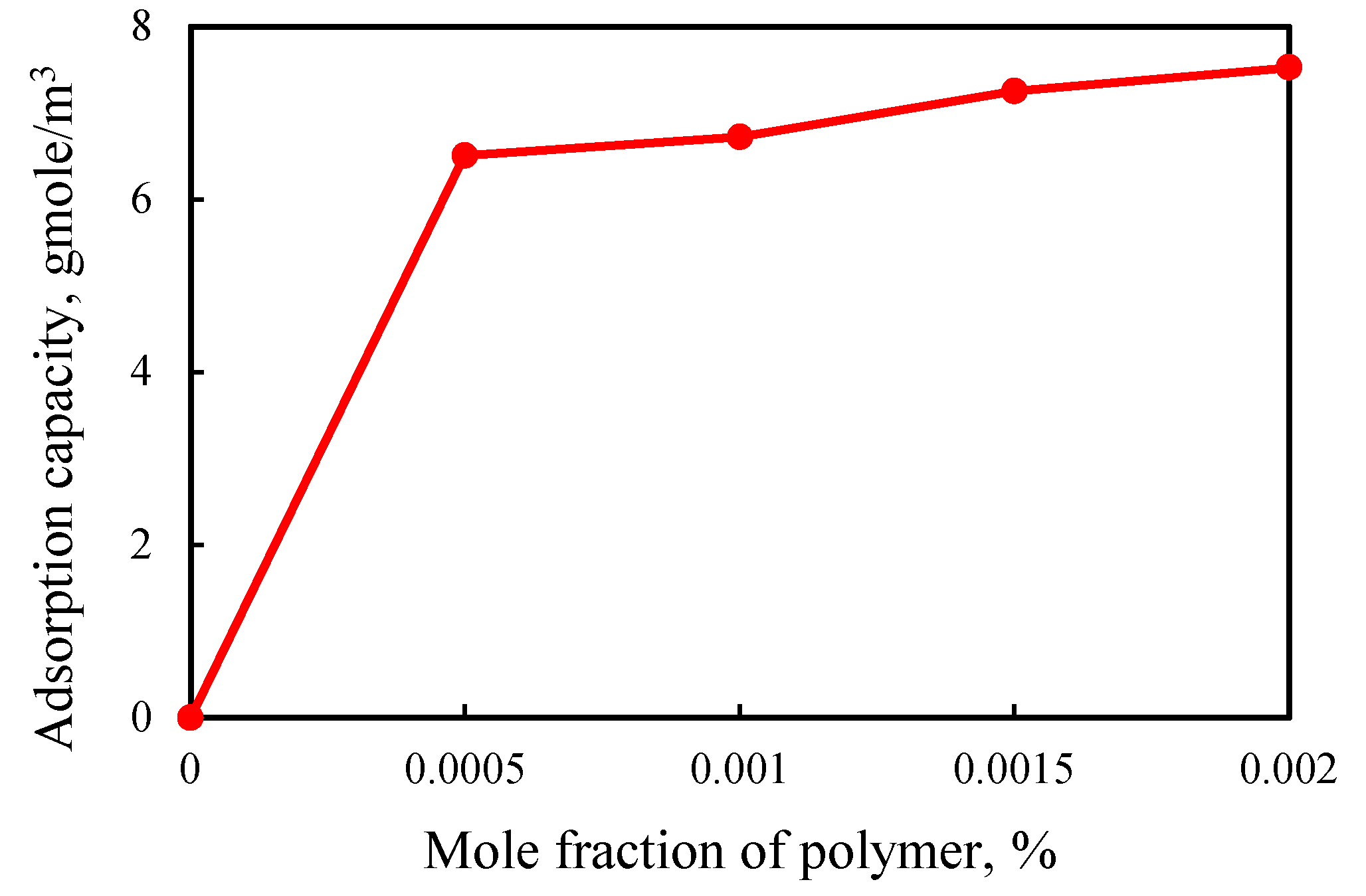
(2): Polymer adsorption

During polymer flooding processes, the polymer is easily attracted to the rock surface under the action of physical forces. The polymer adsorption as the most important mechanism should be considered in the model because the polymer concentration in the solution decreases when polymer adsorption is obvious. The Langmuir isotherm was used to calculate the polymer adsorption as follows [37]:

A d = \frac{a + (b \times x_{s}) \times x_{p}}{1 + c \times x_{p}}

(18)

where Ad is the polymer adsorption capacity, gmol/m³; x_s denotes the salinity, ppm; a, b, and c are the parameters of Langmuir isotherm, which can be obtained by matching polymer adsorption data.

(3): Permeability reduction

The aqueous phase’s permeability decreases due to the polymer adsorption. The extent of permeability reduction depends on many factors such as the polymer concentration, salinity, and rock properties. For CMG-STARS, the polymer adsorption which may result in the reduction of effective permeability is given by:

k_{e} = \frac{k \times k_{r w}}{R_{k}}

(19)

R_{k} = 1 + (R R F - 1) \times \frac{A D}{A D_{MAX}}

(20)

where k is the standard block permeability, μm²; k_e is the standard block effective water permeability, μm²; k_rw is the water’s relative permeability; R_k means the water’s permeability reduction factor; AD_MAX stands for the maximum adsorption capacity of the rock, gmole/m³; AD denotes the adsorption isotherm; RRF denotes the residual resistance factor which is determined by the experiments.

(4): Inaccessible pore volume (IPV)

The IPV refers to the small pores that remain inaccessible to the polymer solution [38]. The IPV commonly ranges between 10% to 30% of the total pore volume, which depends on the type of rock and polymer [39].

(5): Polymer degradation

Polymer degradation commonly occurs in oil reservoirs due to the rock shear action or other chemical reactions. The equation describing the polymer degradation phenomena is given as follows:

a Polymer \to b Water

(21)

r r f = \frac{\ln 2}{T_{1 / 2}}

(22)

where a and b are the reaction constants; T_1/2 is the polymer solution’s half-life, days; rrf is the reaction rate, 1/ day.

Table 2, Figure 3 and Figure 4 show the values of fluid properties, polymer adsorption data, and relative permeability curves used in the fluid model.

Table 2. The parameter values used in the reservoir simulation model.

Reservoirparameters	Values
Reservoir middle depth (m)	1195
Average porosity (%)	31
Average permeability (mD)	1083
Average oil saturation (%)	63
Initial pressure (MPa)	10.99
Temperature (°C)	58
Fluid parameters	Values
Oil density (kg/m³)	850
Oil viscosity (mPa·s)	2.1478
Water density (kg/m³)	900
Water viscosity (mPa·s)	1
Polymer density (kg/m³)	1000
Polymer molecular weight (kg/mole)	9.5
T_1/2 (day)	750
Rock and fluid interaction parameters	Values
Rock compressibility (1/kPa)	10 e⁻⁴
RRF	1.25
IPV	0.25
AD_MAX (gmole/m³)	7.53

For the offshore oil reservoir, there were 5 production wells and 3 injection wells. All the production wells operated under a bottom-hole pressure of 3.45 MPa and the maximum injection rates for the injection wells were 150 STBD. The cumulative oil production of the 5 production wells was 8.1 × 10⁵ m³ and the cumulative volume of injected water of 3 injection wells was 2.54 × 10⁶ m³ after 8 years of waterflooding. The oil production and water injection data of all the production and injection wells were inputted into the model to restore the production and injection history of the reservoir. A history-matching process was conducted to ensure the reliability of the parameters in the developed model, which provided a reliable platform for subsequent infill well placement optimization processes.

In this study, the HS-AOA was used to optimize simultaneously the numbers of infill production and injection wells and their placements (i, j, and k coordinates) for polymer flooding processes. In addition, two types of infill wells (vertical and horizontal wells) were considered in the optimization processes. The offshore oil reservoir was assumed to drill a maximum of 5 production wells and 5 injection wells, respectively. In addition, all the infill vertical wells were assumed to have perforations in all three layers and the length of all the infill horizontal wells was assumed to be 250 m.

3.2. Results and Discussion

The HS–AOA and AOA were used to find the optimal infill well placement for polymer flooding and their performance were compared. Table 3 presents the parameters utilized in the HS–AOA and AOA.

Figure 5 demonstrates the changes in the NPV values of the polymer flooding with infill wells determined by the HS–AOA and AOA. As illustrated in Figure 5, the NPV values increase as the iteration numbers increase. The NPV values of the polymer flooding with infill wells determined by HS-AOA (the infill well case (HS-AOA)) are larger than those of the polymer flooding with infill wells determined by the basic AOA (the infill well case (AOA)). After 10 iterations, the infill well case (HS-AOA) achieved the highest NPV (3.5 × 10⁸ $).

Figure 5 also indicates that the infill well case (AOA) achieved the highest NPV when the iteration number is 6. However, the infill well case (HS-AOA) achieves the highest NPV when the iteration number is 8. The aforementioned results showed that basic AOA was easily trapped into the local optimal solution while the HS-AOA avoided trapping into local optimal solution and effectively found the globally optimal solution.

Table 4 gives detailed information on the optimal infill well case (HS-AOA). As shown in Table 4, the optimal numbers of infill wells for the polymer flooding are four (1 injection well and 3 production wells), which provides the theoretical basis for practical implementation

Figure 6 illustrates the optimization process for the placement of the infill injection well 1 and the infill production well 1.

As displayed in Figure 6a, the infill injection well 1 gradually moves to the edge area of the reservoir where the water did not displace during the water flooding process. In this case, the infill injection well 1 could improve the sweep range of the polymer flooding. Simultaneously, as the increase of iteration number, the infill production well 1 gradually moves to the placement with high residual oil saturations (Figure 6b), which was beneficial for improving its oil production performance. All the aforementioned results indicated that the HS-AOA is an effective method for determining the optimal infill well placement for polymer flooding, maximizing the NPV values.

Figure 7 presents the performances of the polymer flooding case with the optimal infill well case (HS–AOA), and the optimal infill well case (AOA). As shown in Figure 7b, the oil recovery factors (ORF) of the two optimal infill well cases are higher than that of the polymer flooding case. This observation could be attributed to the better performance of the infill wells. The infill injection well had a significant effect on the flow direction of the polymer, leading to an improved sweep efficiency (Figure 6c). Simultaneously, the 3 infill production wells were located in areas with high residual oil saturations, leading to a high oil production rate, which resulted in the decrease of water cut (Figure 6b) and residual oil saturation (Figure 6d). Therefore, the NPV values of the optimal infill well case (HS–AOA) and the optimal infill well case (AOA) are higher than that of the polymer flooding case (Figure 7a). Specially, the NPV value of the optimal infill well case (HS–AOA) reached 3.5 × 10⁸ $, which was an increase of 7% over that of the polymer flooding case. Therefore, infill drilling is an economical method for improving polymer flooding performance.

Figure 7 also demonstrates that the NPV value of the optimal infill well case (HS–AOA) increases by 0.1 × 10⁸ $ compared to the NPV value of the optimal infill well case (AOA). With regards to the water cut, it was found that the water cut of the optimal infill well case (HS–AOA) was lower than that of the optimal infill well case (AOA). The better performance of the optimal infill well case (HS–AOA) indicated the rationality of infill well placements which resulted in a larger sweep area and lower residual oil saturations shown in Figure 7c,d. The aforementioned results proved the developed HS–AOA’s superiority compared to the basic AOA, which could be attributed to the introduction of the Halton sequence into the AOA, which effectively increased the diversity of the initial objects in the AOA and avoided the HS-AOA trapping into the local optimal solutions.

5. Conclusions

In this study, an improved archimedes optimization algorithm with Halton sequence (HS–AOA) was proposed to optimize the infill well placement for polymer flooding. The codes were developed in MATLAB and connected to a commercial reservoir simulator CMG STARS to carry out the infill well placement optimization. The HS-AOA was compared to the basic AOA to confirm its reliability and then used to optimize the infill well placements for polymer flooding in a typical offshore oil reservoir. The results showed that the introduction of the Halton sequence into AOA effectively increased the diversity of the initial objects in the AOA and avoided the HS-AOA trapping into the local optimal solutions. The HS–AOA outperformed the AOA. It was an effective approach to optimize the infill well placement for polymer flooding processes. In addition, infill drilling could effectively and economically improve the polymer flooding performance in offshore oil reservoirs. The NPV of the polymer flooding case with infill wells determined by HS-AOA reached 3.5 × 10⁸ $, which was an increase of 7% over that of the polymer flooding case. This study presents an effective method for optimizing infill well placement for polymer flooding processes. It also can serve as a valuable reference for other optimization problems in the petroleum industry, such as joint optimization of well control and placement.

Author Contributions

Conceptualization, J.Z.; Methodology, E.T.; Validation, L.L.; Investigation, J.C. and B.H.; Resources, Y.J.; Writing—original draft, A.X.; Writing—review & editing, X.S.; Supervision, X.S. All authors have read and agreed to the published version of the manuscript.

Funding

This research was funded by the Key Technologies R&D Program of CNOOC (KJGG2021-0504) and CNOOC Research Institute Limited’s research and development project (No. CCL2022RCPS0553RSN).

Data Availability Statement

The original contributions presented in the study are included in the article, further inquiries can be directed to the corresponding authors.

Conflicts of Interest

Authors Engao Tang, Jian Zhang, Yi Jin and Lezhong Li were employed by the company CNOOC Research Institute Limited. The remaining authors declare that the research was conducted in the absence of any commercial or financial relationships that could be construed as a potential conflict of interest.

References

Pope, G.A. Recent developments and remaining challenges of enhanced oil recovery. J. Pet. Technol. 2011, 63, 65–68. [Google Scholar] [CrossRef]
Sheng, J.J.; Leonhardt, B.; Azri, N. Status of polymer-flooding technology. J. Can. Pet. Technol. 2015, 54, 116–126. [Google Scholar] [CrossRef]
Wang, D.; Cheng, J.; Xia, H.; Li, Q.; Shi, J.P. Viscous-elastic fluids can mobilize oil remaining after water-flood by force parallel to the Oil-Water interface. In Proceedings of the SPE Asia Pacific Improved Oil Recovery Conference, Kuala Lumpur, Malaysia, 8–9 October 2001. [Google Scholar]
Wei, B.; Romero-Zerón, L.; Rodrigue, D. Oil displacement mechanisms of viscoelastic polymers in enhanced oil recovery (EOR): A review. J. Pet. Explor. Prod. Te. 2014, 4, 113–121. [Google Scholar] [CrossRef]
Morel, D.C.; Vert, M.; Jouenne, S.; Gauchet, R.; Bouger, Y. First polymer injection in deep offshore field Angola: recent advances in the Dalia/Camelia field case. Oil Gas Facil. 2012, 1, 43–52. [Google Scholar] [CrossRef]
Morel, D.; Jouenne, S.; Zaugg, E.; Bouger, Y. EOR polymer in deep offshore field Angola: development strategy and polymer performance surveillance. In Proceedings of the20th World Petroleum Congress, Doha, Qatar, 4 December 2011. [Google Scholar]
Seright, R.S. How much polymer should be injected during a polymer flood? Review of previous and current practices. SPE J. 2017, 22, 1–18. [Google Scholar]
Rathinasamy, M.; Chandramouli, S.; Phanindra, K.B.V.N. Estimation of reservoir storage using artificial neural network. In Proceedings of theWater Resources and Environmental Engineering, Springer, SG, 2 September 2018. [Google Scholar]
Dovan, H.T.; Hutchins, R.D.; Terzian, G.A. Dos cuadras offshore polymer flood. In Proceedings of the SPE California Regional Meeting, Ventura, CA, USA, 4–6 April 1990. [Google Scholar]
Pan, G.M.; Zhang, L.; Huang, J.; Li, H.; Qu, J.F. Twelve years field applications of offshore heavy oil polymer flooding from continuous injection to alternate injection of polymer-water. In Proceedings of the Offshore Technology Conference Asia, Kuala Lumpur, Malaysia, 2–6 November 2020. [Google Scholar]
Wang, J.; Song, L.; Song, K.; Dong, C.; Tian, L.; Chen, G. A Study on the Water/Polymer Co-Flooding Seepage Law and Reasonable Polymer Injection Volume in Offshore Oilfields. Processes. 2020, 8, 515. [Google Scholar] [CrossRef]
Wang, X.; Haynes, R.; Feng, Q. A multilevel coordinate search algorithm for well placement, control and joint optimization. Comput. Chem. Eng. 2016, 95, 75–96. [Google Scholar] [CrossRef]
Yeten, B.; Durlofsky, L.J.; Aziz, K. Optimization of nonconventional well type. SPE J. 2008, 03, 200–210. [Google Scholar]
Güyagüler, B.; Horne, R.N.; Rogers, L.; Rosenzweig, J.J. Optimization of well placement in a gulf of mexico waterflooding project. SPE Reserv. Eval. Eng. 2002, 05, 229–236. [Google Scholar] [CrossRef]
Bouzarefrkounas, Z.; Didier, Y.D.; Auger, A. Well placement optimization with the covariance matrix adaptation evolution strategy and meta-models. Comput. Geosci. 2012, 16, 75–92. [Google Scholar] [CrossRef]
Carosio, G.L.C.; Humphries, T.D.; Haynes, R.D.; Farquharson, C.G. A closer look at differential evolution for the optimal well placement problem. In Proceedings of the 2015 Annual Conference on Genetic and Evolutionary Computation, New York, USA, 11-15 July 2015. [Google Scholar]
Yu, W.; Sepehrnoori, K. An efficient reservoir-simulation approach to design and optimize unconventional gas production. J. Can. Pet. Technol. 2014, 53, 109–121. [Google Scholar] [CrossRef]
Singh, H.; Srinivasan, S. Uncertainty analysis by model selection technique and its application in economic valuation of a large field. In Proceedings of theNorth Africa Technical Conference and Exhibition, Cairo, EGY, 15 April 2013. [Google Scholar]
Singh, H.; Srinivasan, S. Scale up of reactive processes in heterogeneous media-numerical experiments and semi-analytical modeling. In Proceedings of the Improved Oil Recovery Conference, Oklahoma, USA, 12 April 2014. [Google Scholar]
Atashnezhad, A.; Wood, D.A.; Fereidounpour, A.; Khosravanian, R. Designing and optimizing deviated wellbore trajectories using novel particle swarm algorithms. J. Nat. Gas. Sci. Eng. 2014, 21, 1184–1204. [Google Scholar] [CrossRef]
Humphries, T.D.; Haynes, R.D. Joint optimization of well placement and control for nonconventional well types. J. Pet. Sci. Eng. 2015, 12, 242–253. [Google Scholar] [CrossRef]
Emerick, A.; Almeida, L.; Szwarcman, D.; Pacheco, M.A.; Vellasco, M. Well placement optimization using a genetic algorithm with nonlinear constraints. In Proceedings of the Reservoir Simulation Conference, Texas, USA, 2 February 2009. [Google Scholar]
Montes, G.; Bartolome, P.; Udias, A.L. The use of genetic algorithms in well placement optimization. In Proceedings of the SPE Latin American and Caribbean Petroleum Engineering Conference, Buenos Aires, ARG, 25 March 2001. [Google Scholar]
Awotunde, A.A. On the joint optimization of well placement and control. In Proceedings of theSPE Saudi Arabia section technical symposium and exhibition, Al-Khobar, SAU, 21 April 2014. [Google Scholar]
Onwunalu, J.; Durlofsky, L. Application of a particle swarm optimization algorithm for determining optimum well location and type. Comput. Geosci. 2010, 14, 183–198. [Google Scholar] [CrossRef]
Dossary, M.A.A.; Nasrabadi, H. Well placement optimization using imperialist competitive algorithm. J. Pet. Sci. Eng. 2016, 147, 237–248. [Google Scholar] [CrossRef]
Hamida, Z.; Azizi, F.; Saad, G. An efficient geometry-based optimization approach for well placement in oil fields. J. Petrol. Sci. Eng. 2017, 149, 383–392. [Google Scholar] [CrossRef]
Khoshneshin, R.; Sadeghnejad, S. Integrated well placement and completion optimization using heuristic algorithms: A case study of an Iranian carbonate formation. J. Chem. Pet. Eng. 2018, 52, 35–47. [Google Scholar]
Janiga, D.; Czarnota, R.; Stopa, J.; Wojnarowski, P. Self-adapt reservoir clusterization method to enhance robustness of well placement optimization. J. Pet. Sci. Eng. 2019, 173, 37–52. [Google Scholar] [CrossRef]
Hashim, F.A.; Hussain, K.; Houssein, E.H.; Mabrouk, M.S.; Al-Atabany, W. Archimedes optimization algorithm: a new metaheuristic algorithm for solving optimization problems. Appl. Intell. 2021, 51, 1531–1551. [Google Scholar] [CrossRef]
Abualigah, L.; Diabat, A.; Mirjalili, S.; Abd Elaziz, M.; Gandomi, A.H. The arithmetic optimization algorithm. comput. methods, Appl Mech Eng, 2021, 376, 113609. [Google Scholar] [CrossRef]
Khan, R.A.; Farooqui, S.A.; Sarwar, M.I.; Ahmad, S.; Tariq, M.; Sarwar, A.; Zaid, M.; Ahmad, S.; Shah Noor Mohamed, A. Archimedes optimization algorithm based selective harmonic elimination in a cascaded h-bridge multilevel inverter. Sustainability. 2021, 14, 310. [Google Scholar] [CrossRef]
Bouzarkouna, Z.; Ding, D.; Auger, A. Well placement optimization with the covariance matrix adaptation evolution strategy and meta-models. Comput. Geosci. 2012, 16, 75–92. [Google Scholar] [CrossRef]
Jesmani, M.; Bellout, M.C.; Hanea, R. Foss, B. Well placement optimization subject to realistic field development constraints. Comput. Geosci. 2016, 20, 1185–1209. [Google Scholar] [CrossRef]
Michalewicz, Z. A survey of constraint handling techniques in evolutionary computation methods. Evol. Program. 1995, 4, 135–155. [Google Scholar]
Zhang, P.; Tan, X.; Yang, R.; Yang, R.F.; Zheng, W.; Zhang, X.L.; Xie, H.J.; Sun, X.F. Numerical simulations of nitrogen foam and gel-assisted steam flooding for offshore heavy oil reservoirs. J. Porous Media. 2023, 26, 17–32. [Google Scholar] [CrossRef]
Gao, S.L.; Chen, Y.; Wang, X.; Li, S.Q.; Yan, S.G.; Hou, B.F. Research on dynamic performance of anti-polymer adsorbent in Henan oilfield. Dangdai Huagong 2021, 50, 2170–2175. (In Chinese) [Google Scholar]
Al-Shalabi, E.W.; Alameri, W.; Hassan, A.M. Mechanistic modeling of hybrid low salinity polymer flooding: Role of geochemistry. J. Pet. Sci. Eng. 2022, 210, 110013. [Google Scholar] [CrossRef]
Tellez Arellano, A.G.; Hassan, A.M.; Al-Shalabi, E.W.; AlAmeri, W.; Kamal, M.S.; Patil, S. An extensive evaluation of different reservoir simulators used for polymer flooding modeling. In Proceedings of the Gas & Oil Technology Showcase and Conference, Dubai, UAE, 13 March 2023. [Google Scholar]

Figure 1. Flowchart of HS-AOA.

Figure 2. The geologic model of the typical offshore oil reservoir: (a) the oil saturation distributions, (b) the reservoir porosity distributions, and (c) the reservoir permeability distributions.

Figure 3. The polymer adsorption data used in the fluid model.

Figure 4. (a) The water and oil’s relative permeability curves and (b) fluid and gas’s relative permeability curves.

Figure 5. Comparisons of the change of NPV between HS–AOA and AOA.

Figure 6. The optimization processes of the placements of (a) the infill injection well 1 and (b) the infill production well 1 (The background figure is residual oil saturation distributions at the end of the waterflooding process).

Figure 7. The performance of the polymer flooding case, the optimal infill well case (HS–AOA), and the optimal infill well case (AOA): (a) NPV, (b) ORF and water cut, (c) polymer streamline distributions, and (d) the residual oil saturation distributions at the end of the polymer flooding processes.

Table 3. Parameters utilized in the HS-AOA and AOA.

Parameters	Values
N	10
t_max	10
C₁	2
C₂ and C₃	3
C₄	5

Table 4. Detailed information on the optimal infill well case (HS-AOA).

Well name	Well type	Perforation		i	j	z
Well name	Well type	Form (m)	To (m)	i	j	z
Infill injection well 1	Vertical	1181	1191	20	33	1
				20	33	2
				20	33	3
	Horizontal	1189	1196	37	33	1
				38	34	1
Infill production well 1				39	35	1
				40	36	2
				41	37	2
	Horizontal	1209	1212	43	28	2
				44	29	1
Infill production well 2				45	30	2
				46	31	2
				47	32	2
	Horizontal	1193	1195	27	28	1
				28	29	1
Infill production well 3				29	30	1
				30	31	2
				31	32	2

Disclaimer/Publisher’s Note: The statements, opinions and data contained in all publications are solely those of the individual author(s) and contributor(s) and not of MDPI and/or the editor(s). MDPI and/or the editor(s) disclaim responsibility for any injury to people or property resulting from any ideas, methods, instructions or products referred to in the content

© 2024 by the authors. Licensee MDPI, Basel, Switzerland. This article is an open access article distributed under the terms and conditions of the Creative Commons Attribution (CC BY) license (http://creativecommons.org/licenses/by/4.0/).

Copyright: This open access article is published under a Creative Commons CC BY 4.0 license, which permit the free download, distribution, and reuse, provided that the author and preprint are cited in any reuse.

MDPI Initiatives

Important Links

Choose an area of interest and we will send you notifications of new preprints at your preferred frequency.

Disclaimer

Infill Well Placement Optimization for Polymer Flooding in Offshore Oil Reservoirs Using an Improved Archimedes Opti-Mization Algorithm with Halton Sequence

Abstract

1. Introduction

2. Methodology

2.1. Improved AOA with Halton Sequence

2.2. Objective Function

2.3. Handling Infeasible Solutions

3. Applications and Results

3.1. Reservoir Simulation Model

3.2. Results and Discussion

5. Conclusions

Author Contributions

Funding

Data Availability Statement

Conflicts of Interest

References

MDPI Initiatives

Important Links

Subscribe