1. Introduction
In contemporary society, Global Navigation
Satellite Systems (such as GPS, GLONASS, Galileo, and BeiDou) have become
indispensable tools in people's daily lives. These systems play a crucial role
in various fields including navigation, positioning, the internet of vehicles,
earthquake early warning, and resource management. The precision of satellite
navigation significantly influences the development level of these related
fields. Satellite clock bias (SCB) is a highly significant parameter within
satellite navigation systems, directly impacting the accuracy of navigation
positioning. Therefore, the precise prediction of SCB holds great significance
for enhancing the precision and reliability of satellite navigation systems.
Various methods can be employed for SCB prediction,
which can generally be categorized as follows: the physical modeling (e.g., Quadratic
Polynomial, QP (Wang et al. 2020)), the statistical modeling (e.g., Grey Model -
GM (Cui & Jiao, 2005; Liang et al., 2016), Autoregressive Integrated Moving
Average Model – ARIMA (Xu & Zeng, 2009; Li, 2013; Xi et al., 2014; Zhang et
al., 2022), Kalman Filter Model (Zhu et al., 2008; Davis et al., 2012),
Exponential Smoothing (Wang et al., 2017; Yu et al., 2020), etc.), the machine
learning modeling (e.g., Support Vector Machine - SVM (He et al., 2019), Back
Propagation (BP) Neural Network (Lv et al., 2022), Elman Recurrent Neural
Network (Liang et al. 2022), Wavelet Neural Network - WNN (Ai et al., 2016;
Wang et al., 2016), Radial Basis Function - RBF (Li, 2013; Wang et al., 2014),
Long Short-term Memory Network - LSTM (Huang et al., 2021; He et al., 2023),
etc.), the combined prediction models that integrate multiple single models
(e.g., GM and WNN (Wang et al., 2014), wavelet transform and SVM (Lei et al.,
2014), etc.), as well as some improved models within their own categories (Lu
et al., 2008; Zheng et al., 2008; Wang et al., 2017; Huang et al., 2018; Wang
et al., 2021; Bai et al., 2023; Cai et al., 2024). Each prediction method has
specific characteristics suitable for certain applications but may also exhibit
limitations due to the complex time-frequency characteristics of spaceborne
atomic clocks and susceptibility to external environmental factors. For
instance, as a quadratic polynomial model forecasts clock bias, its predictive
errors escalate notably over longer forecasting horizons rendering it
unsuitable for long-term predictions. The predictive precision of GM is heavily
influenced by its exponential coefficient. ARIMA necessitate stable clock bias
data and are thus ill-suited for long-term forecasting. Kalman filters'
efficacy hinges upon understanding atomic clock operational traits and
stochastic prior knowledge. Exponential Smoothing methods are typically suited
only for short- to medium-term projections, and may underperform with data
exhibiting long-term trends or complex nonlinear relationships. The selection
of kernel function parameters in the SVM prediction model exerts significant
impact on predictive performance, yet determining the optimal parameters poses
challenges. WNN models' network topology is cumbersome to determine. RBF models
prediction suffer from a lack of theoretical foundation regarding determining
sample length, sample size, and intervals between samples. Optimizing
combinatorial weights in combinatorial forecasting models poses difficulties.
The current state of clock bias prediction is characterized by the
diversification of SCB models, but they do not have strong universal
adaptability. Therefore, exploring a combination model with strong adaptability
and high prediction accuracy is a hot direction for future clock bias
forecasting models.
The research on satellite clock prediction
increasingly focuses on deep learning methods based on neural networks (Lu et
al., 2023). This paper introduces a novel SCB prediction model based on
BWO-CNN-BiGRU-Attention for the first time. CNN-BiGRU-Attention is a deep
learning model comprising CNN and BiGRU with an attention mechanism. The model
utilizes a CNN to capture local correlations between different time steps and
share local features across various time points. The BiGRU can effectively
model the time series data in both directions, thereby enabling the model to
capture more comprehensive information. Additionally, the attention mechanism
assigns a corresponding weight to each time step, facilitating automatic
selection of the most crucial time points and features, thus enhancing the
performance and effectiveness of the model. The performance of deep learning
models heavily relies on hyperparameter selection and adjustment. To optimize
model parameter selection, this paper employs the optimization algorithm BWO
for parameter optimization, further enhancing accuracy and robustness.
To validate the effectiveness and applicability of
this new predictive model, 300s precision clock bias data from September 6th to
November 9th in 2023 provided by IGMAS are used for experimentation. The
experimental results demonstrate that for BDS satellite-borne hydrogen atomic clock,
the predicted bias at intervals of 6 hours, 3 days and 15 days are 0.078 ns ,0
.475 ns, and 2 .130 ns, respectively. These values were found to be higher improvement
than CNN-BiGRU-Attention by 31%, 45%, and 66%; higher than CNN-BiGRU by 6%,51%,
and 56%; and higher than BiGRU by32%, 35% and 73% for the respective time
intervals.
The structure of this paper is as follows: Section 2 briefly reviews the basic knowledge
of CNN, BiGRU, Attention mechanism and BWO algorithm. Section 3 constructs a SCB prediction model
based on BWO-CNN-BiGRU-Attention, and Section 4
provides an case analysis.Section 5
summarizes the full text.
2. Basic Knowledge
2.1. Convolutional Neural Network
Convolutional Neural Network (CNN), proposed by
Yann Lecun in 1989, are essentially a multi-layer perceptron and one of the
representative algorithms of deep learning (LeCun et al., 2015). CNN model is
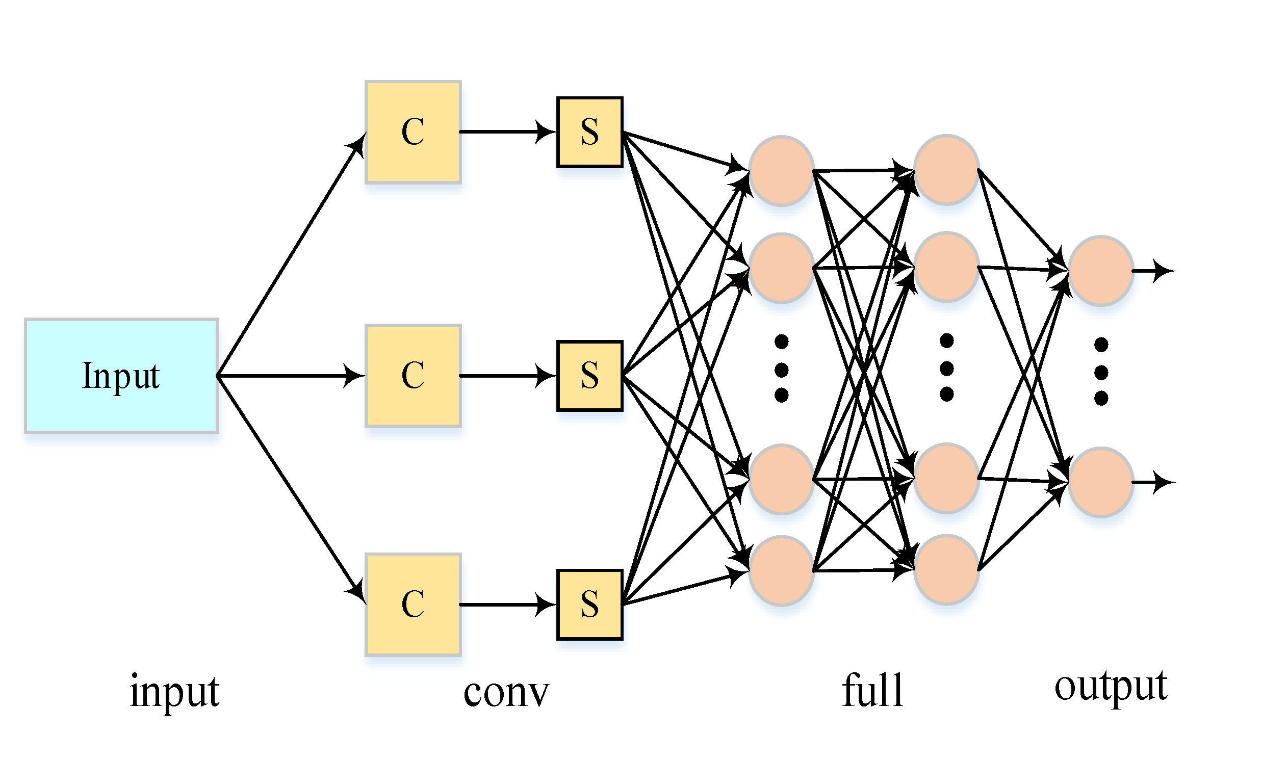
usually composed of input layer, convolution layer, pooling layer, fully
connected layer and output layer, the specific structure is shown in
Figure 1:
Input layer: The input layer serves as the entry
point for the entire network and typically requires preprocessing of the raw
data (the data preprocessing will be covered in Section
3 of this article).
Convolution layer: This layer comprises the
convolution computation and activation layers. The convolution computation
involves matrix operations between the convolution kernel matrix and
corresponding position data matrices, with inputs denoted as , the convolution kernel as , and defined by
, where * represents the convolution operator. The
formula is as follows:
The activation layer functions to nonlinearly transform the output from the convolution computation through an activation function:
Here, denotes a nonlinear activation function, with commonly used options including Sigmoid, tanh, ReLU and their variations.
Pooling layer: The primary purpose of this layer is to compress data, reduce neural network parameters and computations while preventing overfitting. A common pooling method is Max Pooling which utilizes maximum values within pooled areas to highlight key features in data. Other pooling methods include average pooling, overlapping pooling, spatial pyramid pooling , and random pooling (DataCamp, 2024), etc.
Fully connected layer: Neurons in this fully connected layer establish connections with all neurons in preceding layers; its role is to integrate distributed feature representations learned by the network and map them into sample label space.
2.2. Bidirectional Gated Recurrent Unit
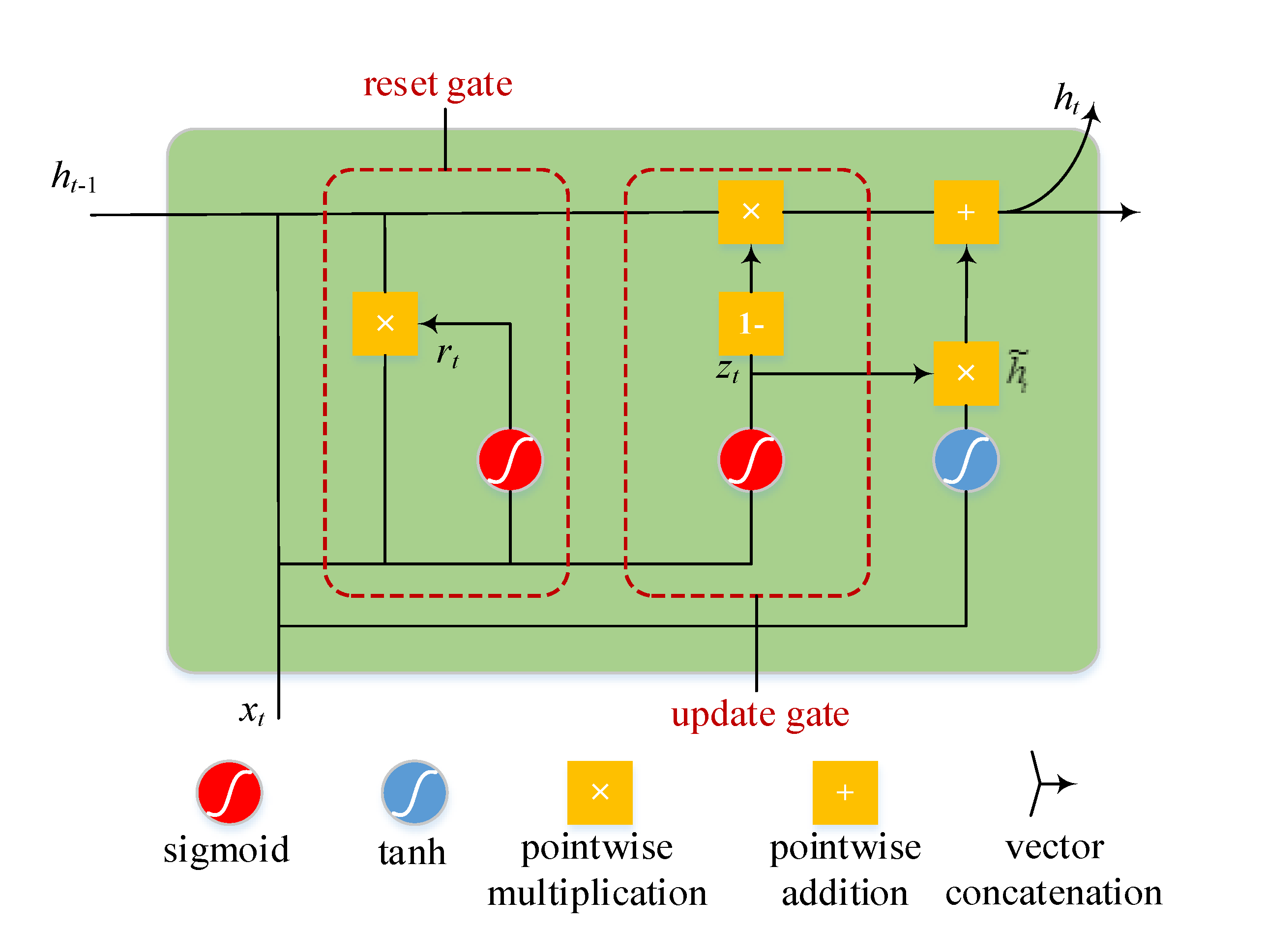
Gated Recurrent Unit (GRU) networks represent an optimization of LSTM networks characterized by simpler model structures that incur lower computational costs while exhibiting improved convergence rates (Cho et al., 2014). The GRU structure is depicted in
Figure 2.
The gated update formula for GRU is as follows:
Where, represents the input vector at time t, and denote the update gate and reset gate. represents the hidden layer state, while signifies the candidate hidden layer state. , , and represent the weight matrix, and , and are bias vector.
However, GRU networks are limited to processing data in a single direction, relying solely on past data for making predictions. In contrast, the Bidirectional Gated Recurrent Unit (BiGRU) network consists of both forward and backward neural networks, enabling it to leverage information from both preceding and subsequent time steps. This allows for more accurate predictions closer to the actual values.
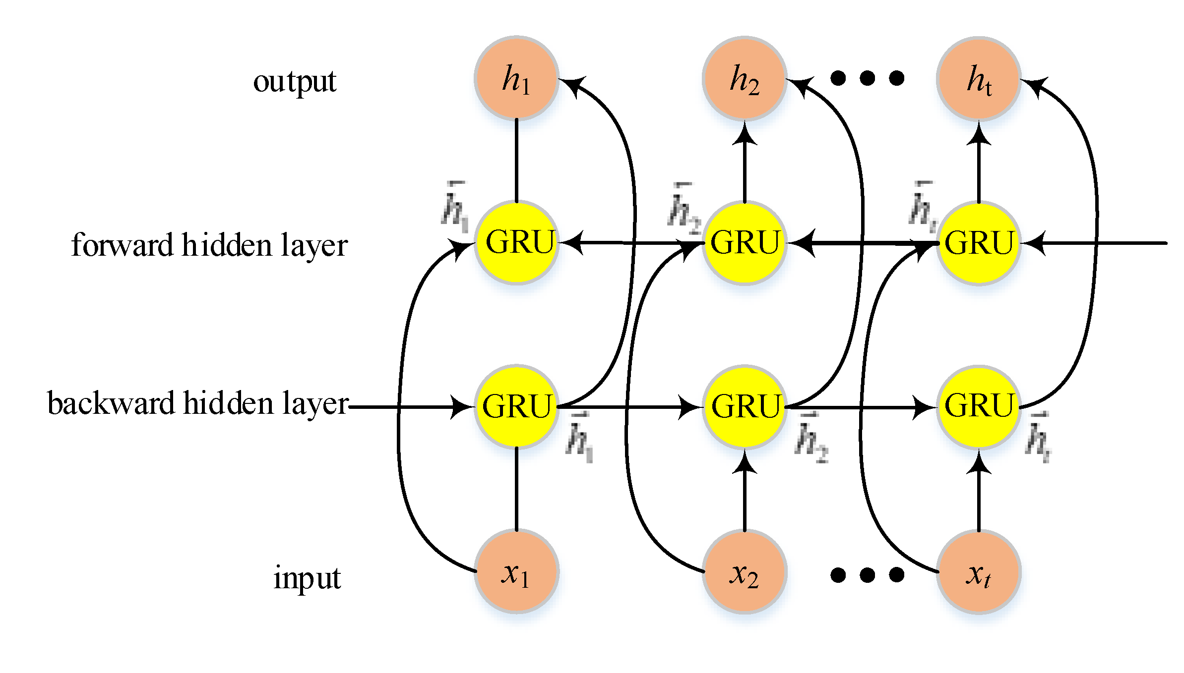
The structure of the BiGRU model is illustrated in
Figure 3 and comprises an input layer, forward hidden layer, backward hidden layer, and output layer. The input layer simultaneously feeds input data into both the forward and backward hidden layers at each time step, facilitating bidirectional flow of data through the GRU network.
At time
t, BiGRU's hidden output is determined by two independent GRUs:
Whereas and represent the output state of the forward GRU and backward GRU at time t, respectively, and represent the weight matrix, and represents the bias vector.
2.3. Attention Mechanism
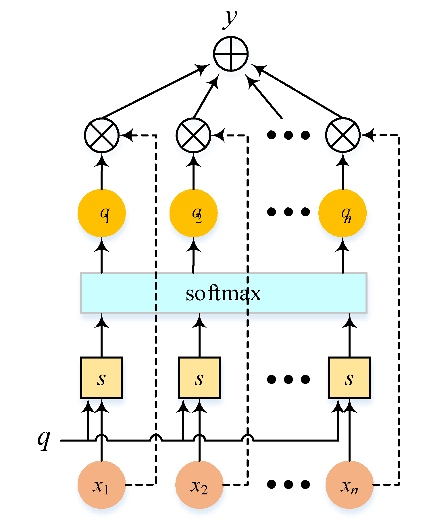
The attention mechanism (Vaswani et al., 2017) simulates human brain resource allocation by focusing attention on specific areas while reducing or ignoring others to obtain relevant information effectively without interference from irrelevant data. The core idea involves assigning different weights based on input data importance for comprehensive focus on crucial parts leading to improved model performance and prediction ability. The Attention structure shown in
Figure 4:
Let
be the input information vector, given a task-related query vector
q, and calculate the attention distribution (weight coefficient)
of the input information:
Where
is the attention score function and softmax is the normalized exponential function.Through softmax processing, the original calculated score is converted into a probability distribution with the sum of ownership weight as 1, which highlights the weight of important elements. The Attention score function s employs various models such as addition model, dot product model, scaled dot product model and bilinear model, etc. In this paper, the addition model is selected:
Where,
,
and
are learnable parameters within neural network. Finally, the Attention layer output y comprises weighted summation of input information using weight coefficients from attention distribution:
2.4. Beluga Whale Optimization
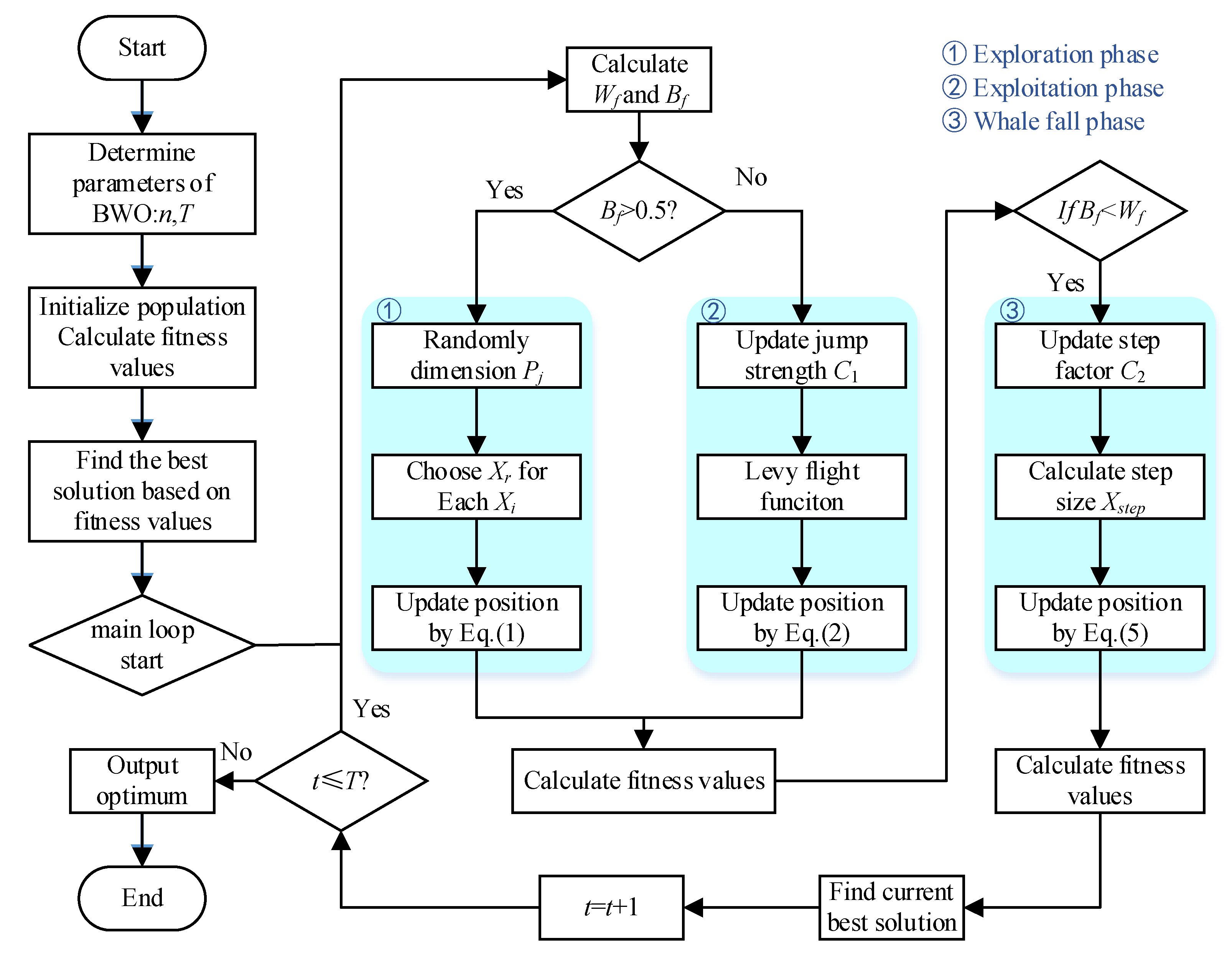
The Beluga Whale Optimization (BWO) algorithm was introduced by Changting Zhong et al in 2022 (Zhong et al., 2022) as a population-based meta-heuristic algorithm designed for numerical optimization and engineering. The algorithm emulates the swimming (Global Exploration), foraging (Local Development), and "whale fall" behaviors of beluga whales, demonstrating strong capabilities in both global and local search. The algorithm flowchart of BWO is shown in Figure5:
The transition from exploration to development is determined based on balance factors:
Where t represents the current iteration, T denotes
the maximum number of iterations, and B0 varies randomly
between (0,1) at each iteration. The equilibrium factor governs the exploration
phase while the
development phase occurs within .
(1) Exploration Phase (Global Exploration)
This stage simulates the swimming behavior of beluga whales through different position updates based on odd-even positions. Its mathematical model is as follows:
Where
t signifies the current number of iterations,
represents the new position of Beluga whale
i on dimension
j,
is randomly selected from dimension
d,
denotes the position of Beluga whale
i on dimension
j, and
and
are respectively current positions of Beluga whales
i and
r (where
r stands for a randomly selected Beluga whale).
r1 and
r2 are random numbers in the range (0,1) that are used to enhance the stochastic operators in the exploration phase.
and
are used to balance the random numbers between the fins.
(2) Development Phase (Local Development)
This stage simulates predatory behavior where belugas move cooperatively to forage based on their surrounding locations. They share location information with each other during hunting to introduce optimal locations along with others. The mathematical model is as follows:
Where
t indicates the current number of iterations;
and
represent current positions of Beluga whale i and a random Beluga whale;
signifies new position for Beluga whale
i;
denotes best position among whales;
r3 and
r4 are random numbers within range (0,1); and
is used to measure the random jump intensity of Levy's flight intensity.
is Levy flight function, which is calculated as follows:
Where and are normally distributed random numbers, and is default constant equaling 1.5.
(3) Whale Fall Phase
During migration or foraging activities, Belugas face threats from killer whales, polar bears, and humans. Most Belugas can escape these threats by sharing information, but some may not survive, falling to deep ocean floors - a phenomenon known as "whale fall." To maintain population size, the updated location is established using Belugas' location combined with length of falling steps. The mathematical model is expressed as:
Where
,
and
represent random numbers between (0,1), and
signifies step length of the whale fall determined as:
Where
is step factor related to probability of whale descent and population size (
),
and
represent upper and lower bounds of variables, respectively. It can be observed that step size is affected by the involved variable, number of iterations, and boundary for maximum number of iterations. In this model, the probability
of whale falling is calculated as a linear function:
3. Development of SCB Prediction Model Based on BWO-CNN-BiGRU-Attention
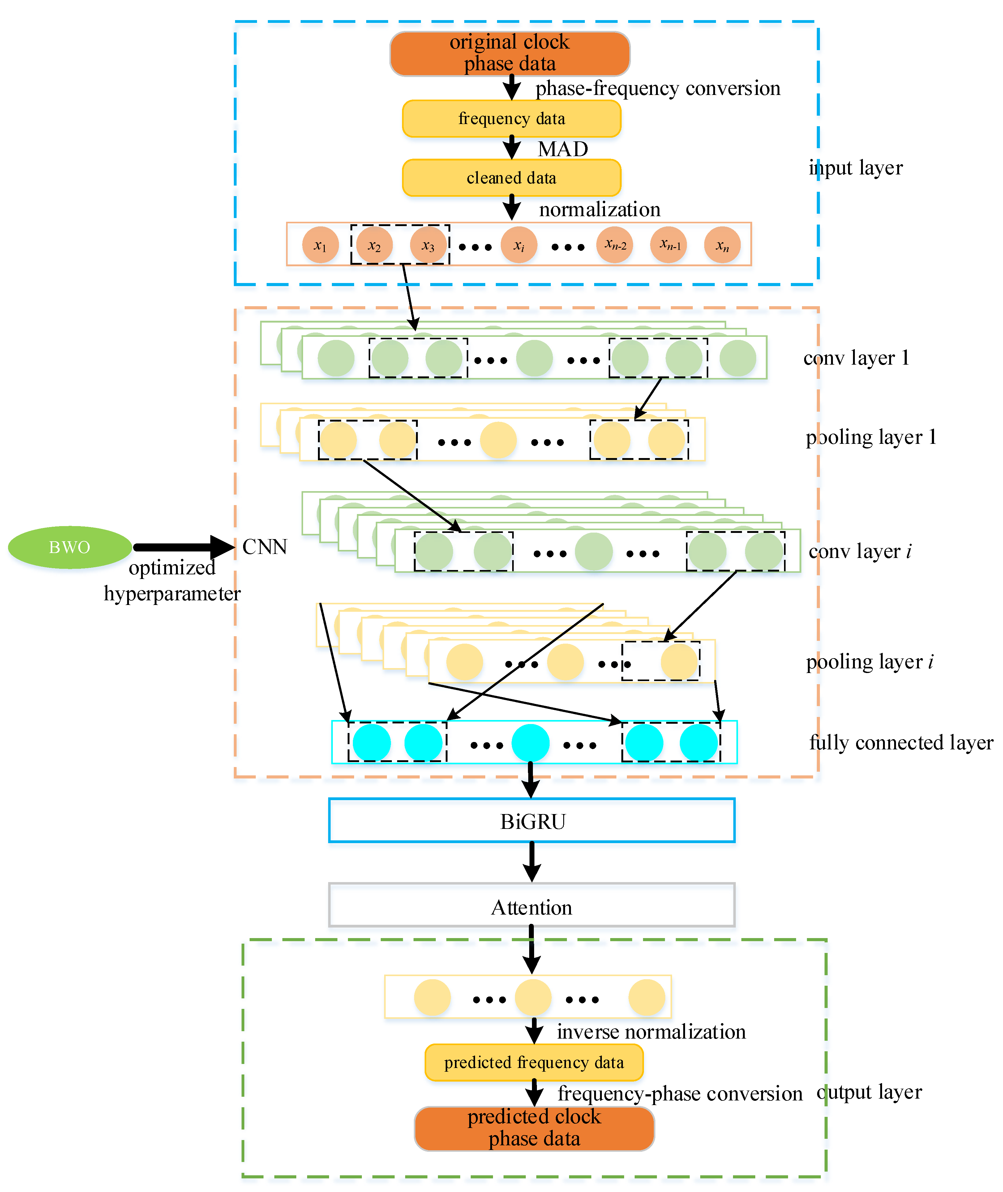
Figure 6 illustrates the construction of a satellite clock bias prediction model based on BWO-CNN-BiGRU-Attention:
(1) Model Input
(a) Data Preprocessing
Addressing outliers in the atomic clock data is crucial. The original phase data may suffer from issues such as missing, jumping, and gross errors, which could significantly impact the accuracy of the clock bias prediction model and its predictive performance. Therefore, preprocessing of the original clock data is essential. Additionally, due to their typically large values on the order of E-4 to E-5, identifying outliers directly from these phase data can be challenging. In this study, we transform the phase data into frequency data and then apply outlier processing techniques (specifically using MAD method) to handle outliers in the frequency data (Huang et al. 2022). Following preprocessing of the frequency data, instead of converting it back into phase data for input into our model, we utilize the frequency data directly for training and predicting purposes. Finally, we convert the predicted frequency data back into phase data.
(b) Data Set Partitioning
The satellite clock bias data set is divided into a training set and a test set. The training set is utilized for model parameter learning, while the test set is employed to assess the predictive accuracy of the model.
(c) Data normalization
The satellite clock bias data undergoes normalization. In the context of machine learning models, data normalization represents a crucial preprocessing step. In this paper, MinMaxScaler is used to carry out data normalization processing, and the input and output features of sample data are mapped to the space of [-1,1], which can remove the impact of data dimension and improve the convergence speed of the model.
Following these operations, the data is fed into the model for training and prediction. CNN is utilized to extract local features, while BiGRU captures long-term dependencies in time series both forward and backward. The attention mechanism preserves essential features to a significant extent, with hyperparameter optimization in the CNN model being performed using the BWO algorithm.
(2) BWO Optimization
The performance of deep learning models heavily relies on hyperparameter selection and adjustment. During model training, the BWO algorithm is employed to optimize and update model hyperparameters such as convolution kernel weight, convolution kernel channel, and fully connected layer.
(3) CNN Layer
Upon obtaining model hyperparameters through the BWO optimization algorithm, these parameters are then returned to train and predict within the CNN model.
(4) BiGUR Layer
The output feature vector from the CNN layer is fed into the BiGRU network, where the BiGRU network, through its forward and backward propagation, stacks the feature information to fully explore the correlations within the clock bias data.
(5) Attention Layer
The feature vectors derived from the BiGRU network's training process are fed into the Attention layer. This layer computes the distribution of attention weights and selectively aggregates the feature vectors based on these weights, thereby accentuating the retention of the most salient features.
(6) Model Output
The Attention layer yields the predicted frequency data of the satellite clock biases. Subsequent frequency-to-phase conversion processes are applied to derive the anticipated phase data of the atomic clocks.
(7) Model Evaluation
The performance of the satellite clock bias prediction model, which integrates BWO-CNN-BiGRU-Attention, is assessed using five key metrics: Root Mean Square Error (RMSE), Mean Absolute Error (MAE), Mean Squared Error (MSE), Mean Absolute Percentage Error (MAPE), and the coefficient of determination R2.
In this context, represents the predicted value of the clock bias, while denotes the actual value of the clock bias, and n is the number of samples. The smaller the values of the model's parameters such as RMSE, MAE, MSE, and MAPE, the better the model's predictive performance. A coefficient of determination, denoted as R2, closer to 1 signifies a higher degree of fit of the model to the sample data, thereby indicative of superior predictive capabilities.
Table 1.
The Evaluation Indicators of SCB Prediction Model.
Table 1.
The Evaluation Indicators of SCB Prediction Model.
| Evaluation Indicators |
Calculation Formula |
How to Evaluate |
RMSE
(Root Mean Square Error) |
|
the lower the value,
the better the model |
MAE
(Mean Absolute Error) |
|
MSE
(Mean Square Error) |
|
MAPE
(Mean Absolute Percentage Error) |
|
R2
(R-Square) |
|
The higher the value,
The better the model |
4. Case Analysis
This paper utilizes the precise 300-second clock bias data of the BeiDou Navigation Satellite System (BDS) provided by the International GNSS Monitoring and Assessment System (IGMAS) (IGS, 2024), spanning from September 6, 2023, to November 9, 2023 - a total of 65 days (denoted as 20230906-20231220) - for experimental validation of the effectiveness and universality of the satellite clock bias forecasting model based on BWO-CNN-BiGRU-Attention.
To fully leverage the aforementioned data, the 65-day dataset is segmented into five intervals of 5 days each, denoted as Segment 1 (20230906-20231020), Segment 2 (20230911-20231025), Segment 3 (20230916-20231030), Segment 4 (20230921-20231104), and Segment 5 (20230926-20231109). For each segment, the first 30 days of clock bias data are employed as the training set to conduct short-term (6 hours), medium-term (3 days), and long-term (15 days) forecasts.
The primary focus of this paper is to evaluate the performance of the BDS satellite clock bias forecasting model using the BWO-CNN-BiGRU-Attention approach. Statistics indicate that the BDS satellites in orbit primarily operate Rb (rubidium) and H (hydrogen) atomic clocks.
Table 2 provides the PRN (Pseudo-Random Noise) codes corresponding to different types of BDS satellite-borne atomic clocks.
Upon analysis, it is found that the GEO (Geostationary Earth Orbit) data from the 65-day BDS clock bias data provided by IGMAS is insufficient, while the IGSO (Inclined Geosynchronous Satellite Orbit) and MEO (Medium Earth Orbit) satellite clock bias data are complete without any missing instances. Consequently, one satellite-borne atomic clock is randomly selected from both the IGSO and MEO for experimentation (PRN27 and PRN40).
Below, taking the clock bias data of PRN27 for the Segment 1 period as an example, the process of using the BWO-CNN-BiGRU-Attention model to forecast 15 days ahead based on 30 days of clock bias data is illustrated.
4.1. Data Preprocessing
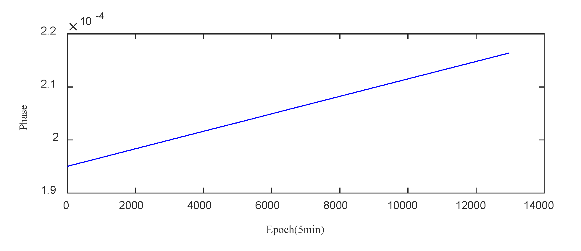
During the period from September 6, 2023, to October 20, 2023, the raw phase data of the PRN27 satellite-borne atomic clock is presented in
Figure 7.
Examination of
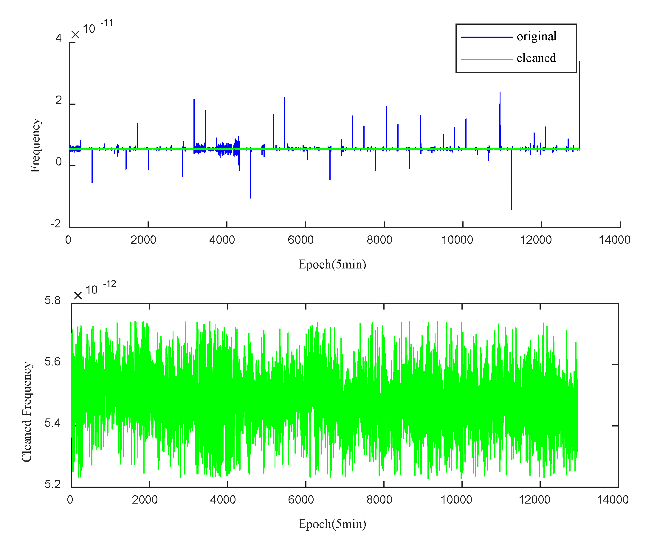
Figure 7 reveals that anomalies are not readily discernible from the raw phase data. To overcome this, a phase-to-frequency transformation is applied to obtain the clock bias frequency data. As shown in
Figure 8 (above), certain outliers within the clock bias data become clearly identifiable. Utilizing the Median Absolute Deviation (MAD) method, outliers in the PRN27 clock bias frequency data are removed, with a threshold factor set to 3. The outliers are then interpolated using a linear interpolation method, as depicted in
Figure 8 (below).
4.2. Training and Prediction with the BWO-CNN-BiGRU-Attention Model
This study employs two 2
×2 convolutional layers and max pooling layers to extract features from satellite clock bias data, with the ReLU function chosen as the activation function for the convolutional layers and max pooling selected for the pooling layers. After processing by the convolutional and pooling layers, the feature vectors are passed through a fully connected layer structure and activated by the Sigmoid function to obtain the final output vector of the CNN layer. Considering the training time, the initial population size of the BWO algorithm is set to
n = 5, with a maximum number of iterations
T = 3, and the model prediction step is set to 10, meaning that the frequency value of the 11th moment is predicted using the frequency values of the preceding 10 moments. The main hyperparameters are set as shown in
Table 3 below:
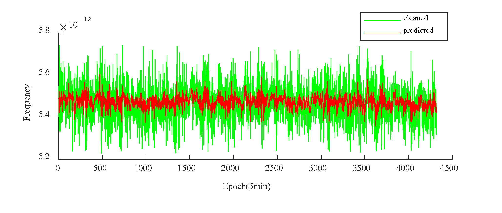
For PRN27, the 15-day frequency prediction results are depicted in
Figure 9:
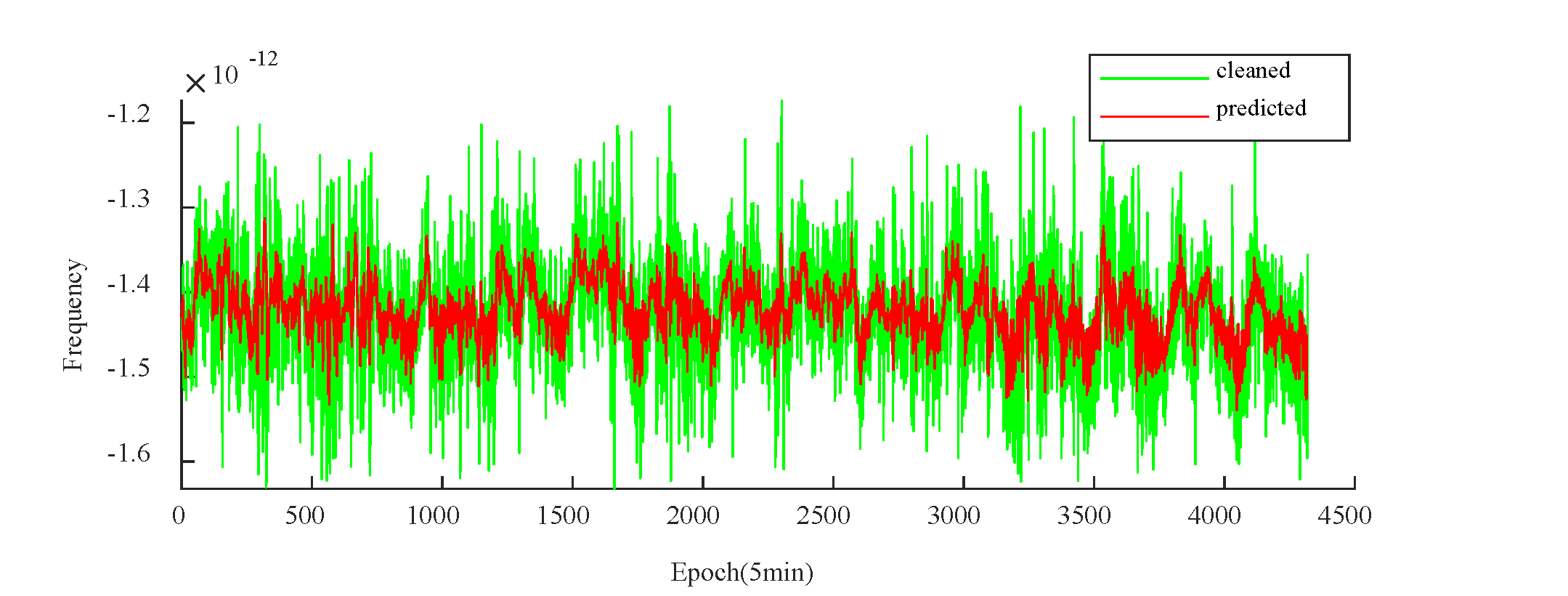
For PRN40, the corresponding 15-day frequency prediction outcomes are illustrated in
Figure 10:
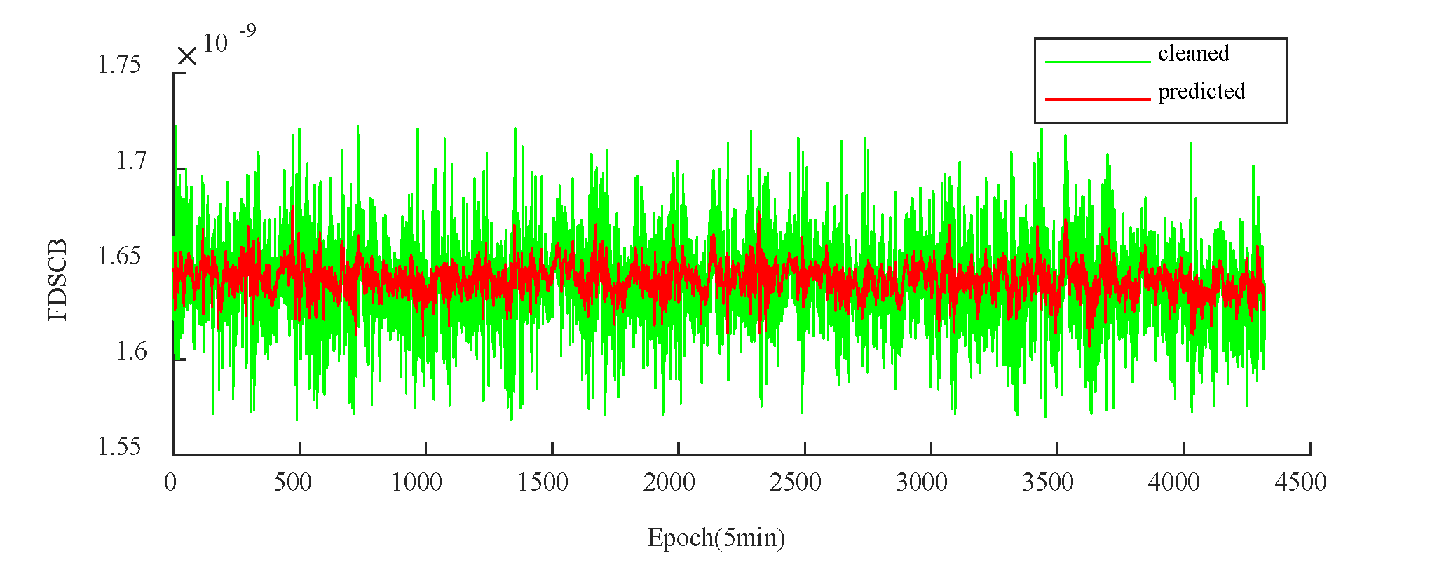
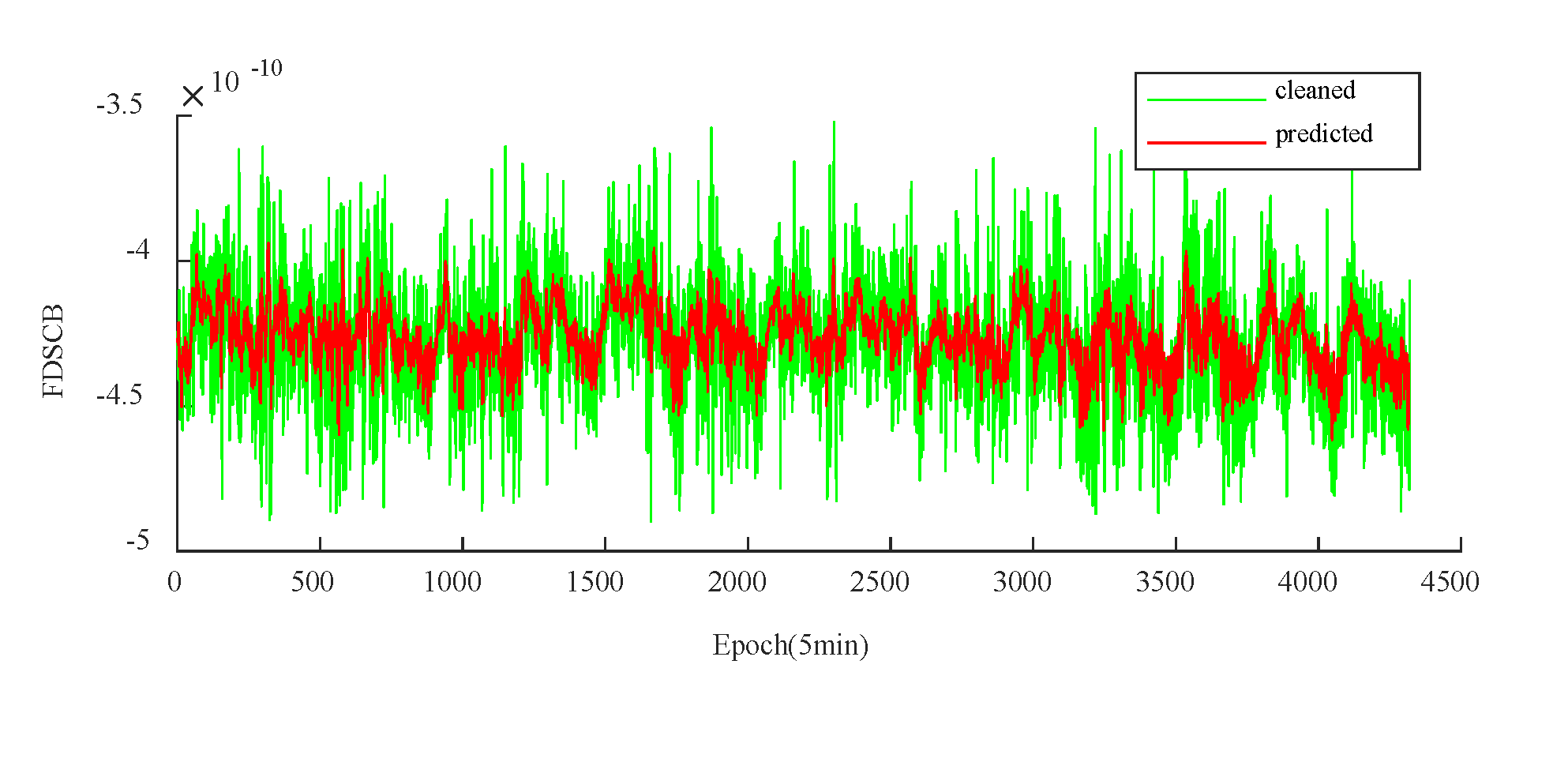
Following the completion of the frequency predictions, the forecasted frequency information is transformed into predicted phase information, with the accuracy of the clock bias predictions determined by RMSE between the actual and predicted phase data.
Figure 11 and
Figure 12 present the first-order differences between the actual and predicted phases for PRN27 and PRN40 over a 15-day period, respectively, where the green line represents the actual first-order phase difference, and the red line indicates the predicted first-order phase difference.
Table 4 presents the clock bias prediction results for two BDS satellites, PRN27 (Hydrogen) and PRN40 (Hydrogen), based on the BWO-CNN-BiGRU-Attention model.
4.3. Results Comparison
To validate the effectiveness of the satellite clock bias prediction using the BWO-CNN-BiGRU-Attention model, this paper compares its performance with that of the CNN-BiGRU-Attention, CNN-BiGRU, and BiGRU models on the same dataset. The average values from five different time segments are used to represent the clock bias prediction results of the models, with the RMSE results detailed in the following
Table 5:
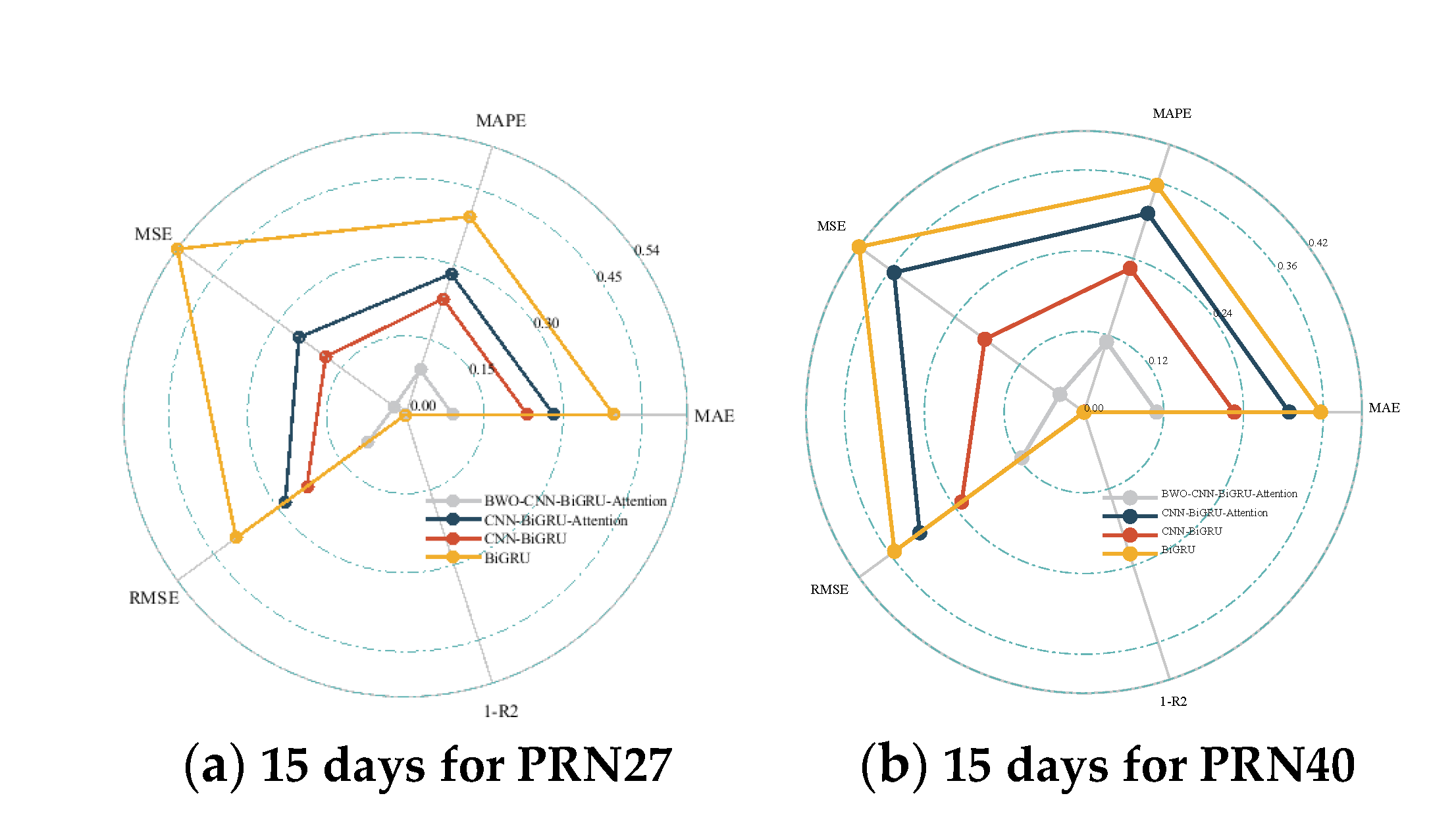
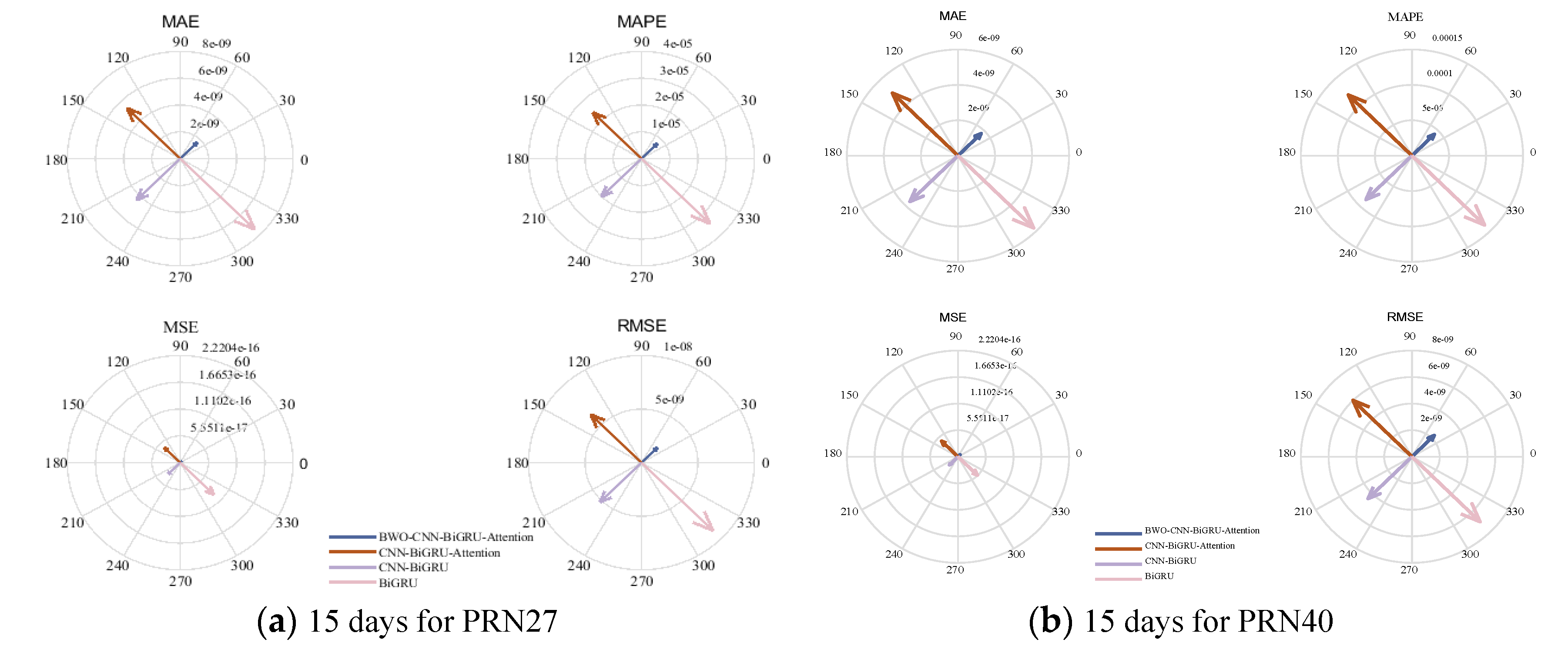
For ease of comparison, each evaluation metric has been normalized to the same dimension. A detailed comparison of the prediction evaluation metrics for the BWO-CNN-BiGRU-Attention, CNN-BiGRU-Attention, CNN-BiGRU, and BiGRU models can be found in
Figure 13 and
Figure 14. Due to space constraints, only the results for the 15-day forecast are presented in the comparative figures. It is evident that the satellite clock bias prediction model based on BWO-CNN-BiGRU-Attention outperforms the others across all metrics.
Additionally, the navigation satellite clock bias prediction model based on the BWO-CNN-BiGRU-Attention framework has also demonstrated optimal performance for 6-hour and 3-day forecasts.
This paper utilizes the average prediction results of PRN27(H) and PRN40(H), two satellites, to represent the predictive outcomes for BDS satellite clock bias across various models. According to the aforementioned calculations, the RMSE results for the 6-hour, 3-day, and 15-day predictions of the satellite clock bias based on the BWO-CNN-BiGRU-Attention model are 0.078 ns, 0.476 ns, and 2.13 ns, respectively. In contrast, the RMSE for the 6-hour, 3-day, and 15-day predictions based on the CNN-BiGRU-Attention model are 0.113 ns, 0.856 ns, and 6.18 ns, respectively. For the CNN-BiGRU model, the RMSE for the same prediction periods are 0.083 ns, 0.981 ns, and 4.84 ns, respectively. Lastly, the BiGRU model yields an RMSE of 0.115 ns, 0.734 ns, and 7.94 ns for the 6-hour, 3-day, and 15-day predictions, respectively.
In summary, the computational outcomes indicate that the satellite clock bias predictions yielded by the BWO-CNN-BiGRU-Attention model are markedly superior to those of the CNN-BiGRU-Attention, CNN-BiGRU, and BiGRU models. Specifically, the model's predictions for the 6-hour, 3-day, and 15-day intervals have demonstrated improvements of 30%, 44%, and 66%, respectively, over the CNN-BiGRU-Attention model. Furthermore, the predictions have shown enhancements of 6%, 51%, and 56%, respectively, when compared to the CNN-BiGRU model. Lastly, in comparison to the BiGRU model, the improvements are 32%, 35%, and 73% for the same prediction intervals. These results underscore the efficacy of the BWO-CNN-BiGRU-Attention model in providing more accurate predictions for satellite clock biases over various time horizons.
5. Conclusions
Satellite clock bias is one of the primary sources of error in satellite navigation and positioning, particularly for real-time applications. The significance of predicting satellite clock bias lies in enhancing the accuracy and timeliness of satellite navigation and positioning systems, thereby providing users with more precise and up-to-date location services. By conducting assessments and forecasting research on satellite clock bias, the precision and reliability of satellite navigation and positioning can be significantly improved.
This paper introduces a novel method for predicting satellite clock bias based on the Beluga Whale Optimization algorithm optimized CNN-BiGRU-Attention model. Experimental results demonstrate that this method offers high predictive accuracy and efficiency. The RMSE for short-term (6-hour), medium-term (3-day), and long-term (15-day) predictions are 0.078 ns, 0.476 ns, and 2.13 ns, respectively. These results are notably superior to those of the CNN-BiGRU-Attention, CNN-BiGRU, and BiGRU models. Future research can further explore the application and refinement of this method to meet the practical demands of navigation systems.
Author Contributions
SWL and CJP proposed the method used in this paper and complete the experiment; HCB, LYX, WML, and ZH discussed and analyzed the experimental results and the manuscript, and proposed suggestions for improvements; ZR, FGT, and ZT discussed and analyzed the data preprocessing of the experimental process and the experimental results. All authors read and approved the final manuscript.
Funding
There is no any funding or project support for this manuscript.
Acknowledgments
Thanks Senior Engineer Shi Fengfeng, Lin Yuting, Xu Jinfeng and Guo Hairong from Beijing Satellite Navigation Center for their discussion and guidance. Thanks to International GNSS Monitoring & Assessment System (
http://www.igmas.org) for providing data support.
Competing Interests: The authors declare that they have no competing interests.
References
- Ai QS, Xu TH, Li JJ, Xiong HW (2016) The short-term forecast of BeiDou satellite clock bias based on wavelet neural network. In: 2016 China Satellite Navigation Conference, pp.145-154. [CrossRef]
- Bai HW, Cao QQ, An SB (2023) Mind evolutionary algorithm optimization in the prediction of satellite clock bias using the back propagation neural network. Scientific Reports 13:2095. [CrossRef]
- Cai CL, Liu MY, Li PC, Li ZX, Lv KH (2024) Enhancing satellite clock bias prediction in BDS with LSTM-attention model. GPS Solutions 28:92. [CrossRef]
- Cho K, Merriënboer BV, Gulcehre C,, Bahdanau D, Bougares F, Schwenk H, Bengio Y (2014) Learning Phrase Representations using RNN Encoder-Decoder for Statistical Machine Translation. In Proceedings of the 2014 Conference on Empirical Methods in Natural Language Processing (EMNLP), pages 1724–1734, Doha, Qatar.
- Cui XQ, Jiao WH (2005) Grey system model for the satellite clock error predicting. Geomatics and Information Science of Wuhan University 30(5):447-450.
- DataCamp (n.d.) An Introduction to Convolutional Neural Networks (CNNs). https://www.datacamp.com/tutorial/introduction-to-convolutional-neural-networks-cnns. Accessed 21st, August, 2024.
- Davis J, Bhattarai S, Ziebart M (2012) Development of a Kalman filter based GPS satellite clock time-offset prediction algorithm. In: 2012 IEEE European Frequency and Time Forum, pp,152-156. [CrossRef]
- He LN, Zhou HR, Liu ZQ, Wen YL, H XF (2019) Improving clock prediction algorithm for BDS-2/3 satellites based on LS-SVM method. Remote Sensing 11(21):2554. [CrossRef]
- He SF, Liu JL, Zhu XW, Dai ZQ, Li D (2023) Research on modeling and predictions of BDS-3 satellite clock bias using the LSTM neural network model. GPS Solutions 27(3):108. [CrossRef]
- Huang BH, Ji ZX, Zhai RJ, Xiao CF, Yang F, Yang BH, Wang YP (2021) Clock bias prediction algorithm for navigation satellites based on a supervised learning long short-term memory neural network. GPS Solutions 25(2):80. [CrossRef]
- Huang BH, Yang BH, Li MG, Guo ZK, Mao JY, Wang H (2022) An improved method for MAD gross error detection of clock error. Geomatics and information science of Wuhan University 47(5):747-752. [CrossRef]
- Huang GW, Cui BB, Zhang Q, Fu WJ, Li PL (2018) An improved predicted model for BDS ultra-rapid satellite clock offsets. Remote Sensing 10(1):60. [CrossRef]
- IGS (2024). Products. http://www.igs.org/products, accessed 14th, May, 2024.
- LeCun Y, Bengio Y, Hinto G (2015) Deep Learning. Nature 521:436-444. [CrossRef]
- Lei Y, Zhao DN, Li B, Gao YP (2014) Prediction of satellite clock bias based on wavelet transform and least square support vector machines. Geomatics and Information Science of Wuhan University 39(7):815-819.
- Li XY, Dong XR, Zheng K, Liu YT (2013) Research of satellite clock error prediction based on RBF neural network and ARMA model. In: 2013 China Satellite Navigation Conference, pp. 325-334. [CrossRef]
- Liang Y, Xu J, Wu M (2022) Elman Neural Network Based on Particle Swarm Optimization for Prediction of GPS Rapid Clock Bias. In: Yang, C., Xie, J. (eds) China Satellite Navigation Conference (CSNC 2022) Proceedings. Lecture Notes in Electrical Engineering, vol 910. Springer, Singapore. [CrossRef]
- Liang YJ, Ren C, Yang XF, Pang GF, Lan L (2016) A Grey model based on first difference in the application of the satellite clock bias prediction. Acta Astronom Sinica 56(3):264-277. [CrossRef]
- Lu XF, Yang ZQ, Jia XL, Cui XQ (2008) Parameter optimization method of gray system theory for the satellite clock error predicting. Geomatics and Information Science of Wuhan University 33(5):492-495.
- Lu YW, Zheng LQ, Hu C (2023) Analysis and comparison of satellite clock error prediction based on various deep learning algorithms. GNSS World of China 48(5):46-55, 91. [CrossRef]
- Lv D, Liu GY, Ou JK, Wang SL, Gao M (2022) Prediction of GPS Satellite Clock Offset Based on an Improved Particle Swarm Algorithm Optimized BP Neural Network. Remoet Sensing 14(10), 2407. [CrossRef]
- Vaswani A, Shazeer N, Parmar N, Uszkoreit J, Jones L, Gomez AN, Kaiser L, Polosukhin I (2017) Attention is all you need. In Proceedings of the 31st International Conference on Neural Information Processing Systems:6000-6010.
- Wang GC, Liu LT, Xu AG, Su XQ, Liang XH (2014) The application of radial basis function neural network in the GPS satellite clock bias prediction. Acta Geodaetica Et Cartographica Sinica 43(8):803-807.
- Wang L, Zhang Q, Huang GW, Tian J (2017) GPS satellite colck bias prediction based on exponential smoothing method. Geomatics and Information Science of Wuhan University 42(7):995-1001. [CrossRef]
- Wang X, Chai HZ & Wang C (2020) A high-precision short-term prediction method with stable performance for satellite clock bias. GPS Solutions 24, 105. [CrossRef]
- Wang X, Chai HZ, Wang C, Xiao GR, Chong Y, Guan XG (2021) Improved wavelet neural network based on change rate to predict satellite clock bias. Survey Review 53(379):325-334. [CrossRef]
- Wang YP, Lv ZP, Chen ZS, Huang LY (2014) A method of satellite clock bias prediction based on grey model and wavelet neural network. Journal of Geodesy and Geodynamics 34(3):155-159.
- Wang YP, Lv ZP, Chen ZS, Huang LY, Li LY, Gong XC (2016) A new data preprocessing method of satellite clock bias and its application in WNN to predict medium-term and long-term clock bias. Geomatics and Information Science of Wuhan University 41(3):373-379. [CrossRef]
- Wang YP, Lu ZP, Qu YY, Li LY, Wang N (2017) Improving prediction performance of GPS satellite clock bias based on wavelet neural network. GPS Solutions 21(2):523-534.
- Xi C, Cai CL, Li SM, Li XH, Li ZB, Deng KQ (2014) Long-term clock bias prediction based on an ARMA model. Chinese Astronomy and Astrophysics 38(3):342-354. [CrossRef]
- Xu JY, Zeng AM (2009) Application of ARIMA (0,2,q) model to prediction of satellite clock error. Journal of Geodesy and Geodynamics 29(5):116-120.
- Yu Y, Huang M, Wang CY, Hu R, Duan T (2020) A new BDS-2 satellite clock bias prediction algorithm with an improved exponential smoothing method. Applied Sciences 10(21):7456. [CrossRef]
- Zhang GC, Han SH, Ye J, Hao RZ, Zhang JC, Li X, Jia K (2022) A method for precisely predicting satellite clock bias based on robust fitting of ARMA models. GPS Solutions 26:3. [CrossRef]
- Zheng ZY, Lu XS, Chen YQ (2008) Improved grey model and application in Real-Time GPS satellite clock bias prediction. In: 2008 Fourth International Conference on Natural Computation, pp. 419-423. [CrossRef]
- Zhong CT, Li G, Meng Z (2022) Beluga whale optimization: A novel nature-inspired metaheuristic algorithm. Knowledge - Based Systems, 5 (251). [CrossRef]
- Zhu XW, Xiao H, Yong SW, Zhuang ZW (2008) The Kalman algorithm used for satellite clock offset prediction and its performance analysis. Journal of Astronautics 29(3):966-970.
|
Disclaimer/Publisher’s Note: The statements, opinions and data contained in all publications are solely those of the individual author(s) and contributor(s) and not of MDPI and/or the editor(s). MDPI and/or the editor(s) disclaim responsibility for any injury to people or property resulting from any ideas, methods, instructions or products referred to in the content. |
© 2024 by the authors. Licensee MDPI, Basel, Switzerland. This article is an open access article distributed under the terms and conditions of the Creative Commons Attribution (CC BY) license (http://creativecommons.org/licenses/by/4.0/).
