1. Introduction
The phenomenon of phase transitions is prevalent both in nature and in everyday life, making it a topic of great interest [
1,
2,
3]. Particularly for lattice models defined on cubic lattices, this subject has captivated many scientists, showing an ever-growing trend in research [
4,
5]. Significant attention has been given to phase transitions in fields such as statistical mechanics and condensed matter physics. Due to the inherent structure of Cayley trees (CTs) and Bethe lattices (BLs), determining the phase transition behavior in lattice models (such as Ising, Potts, and SOS) on these lattices is more straightforward [
6]. This research can provide valuable insights and potentially inspire further studies on cubic lattices. The Potts model is a generalization of the Ising model [
7] used in statistical mechanics to study phase transitions, magnetism, and critical phenomena [
8]. It is particularly useful in understanding systems with more than two possible states at each site, making it applicable to a wide range of physical, chemical, and even biological systems [
9].
The solid-on-solid (SOS) model, a statistical mechanics model, is used to study the behavior of interfaces in materials [
10]. The SOS model on the CT was introduced by Rozikov and Suhov [
11]. In [
10], the scenario of arbitrary conditions is addressed, and a vector-valued functional equation is derived to describe potential boundary laws of the model. Recently, in [
12], Rahmatullaev and Abraev have provided the phase transition problem of the SOS model on the CT and the corresponding classification of Gibbs measures.
As discussed in our previous studies [
13,
14,
15], we employed three primary methods to analyze the thermodynamic properties and phase transition phenomena of lattice models defined on the CTs:
- (1)
Kolmogorov consistency condition,
- (2)
Cavity method (utilizing the self-similarity of the Cayley tree),
- (3)
Transition matrix method.
Recently, structures known as mixed-lattice models have become the focus of extensive research. Consequently, the Potts-SOS model can be viewed as a type of mixed-lattice model. Rahmetullaev et al. [
16] studied the phase transition problem of the Potts-SOS model with the spin set
on the CT using the Kolmogorov consistency condition. In [
13], we demonstrated that there is no phase transition in the 1-D Potts-SOS model with the spin set
and calculated various thermodynamic quantities using the transition matrix method. In this study, we aim to explore the uniqueness and construction of Gibbs measures associated with a mixed-type lattice model, characterized by Potts and SOS Hamiltonians with two distinct coupling constants, using the self-similarity of the second-order semi-infinite CT. To achieve this, we will first define the partial partition functions and then derive the Gibbs measures using the cavity method. To determine the number of these Gibbs measures, we will identify the fixed points of the two-dimensional dynamical system that we construct.
As is well known, the phase transition problem of lattice models on the CT has been a subject of study for a long time [
2,
17]. For a phase transition to occur, the number of Gibbs measures for the given model must exceed one. Generally, determining the exact number of Gibbs measures directly is a challenging problem [
15]. Instead, researchers investigate the fixed points of the dynamical system formed by the iterative equations, as there is a one-to-one correspondence between these fixed points and the Gibbs measures [
6]. Consequently, the existence and uniqueness of fixed points are analyzed to determine the presence of a phase transition for given lattice model. However, identifying all fixed points analytically, especially for high-dimensional dynamical systems, can be difficult [
18,
19].
The presence of repelling fixed points suggests the existence of additional fixed points [
20,
21]. There are several methods to determine whether a fixed point is repelling. One approach is to check if the derivative of the function at the fixed point is greater than one [
22]. Another method involves identifying regions where the largest eigenvalue of the Jacobian matrix associated with the
n-dimensional dynamical system exceeds one [
22,
23].
In our recent investigation, we have analyzed the stability of fixed points to address the phase transition problem for lattice models on CTs [
24,
25]. In this paper, we will employ both methods—examining the derivative and analyzing the eigenvalues of the Jacobian matrix—to determine the regions where phase transitions occur as a function of the coupling constants.
In our previous research, we employed both the boundary field condition [
26,
27] and the self-similarity property [
14,
15,
28,
29] of the CT to derive the partial partition functions for the Potts-SOS model on a uniform one-order CT. Our findings indicated that the partial partition functions obtained through both methods are equivalent, with the self-similarity method proving to be a more straightforward approach compared to the boundary field condition. In the current paper, we will build on this investigation by examining the thermodynamic properties of the Potts-SOS model using the self-similarity approach of the CT. Previous work [
13] established that no phase transition occurs for the Potts-SOS model on a one-order CT, and therefore, on the
lattice. In this study, our goal is to demonstrate the existence of a phase transition by analyzing the partial partition functions associated with the spin set
.
2. Preliminaries and Construction of the Partial Partition Functions
In this section, we introduce key concepts and results that are fundamental to our findings. To avoid redundancy, we will not go into detailed information about CT in this article. Instead, we suggest readers consult relevant literature for more information [
6,
26,
30]. Here, we will briefly outline a few characteristics of the CT. In a CT of order
k, each node is connected to
neighbors, except for the nodes at the boundary (outermost level), which have only one neighbor. The tree is organized into levels, starting with a single root node at the top (level 0), with each subsequent level branching out with
k branches per node. Unlike square or cubic lattices, the CT contains no closed loops or cycles.
Since the vertices of the CT are loopless [
26,
27,
30], the distance between any two vertices
is defined by the number of edges along the path connecting them. If
is the root of the CT, then
represents the distance from the root to the vertex
x, measured by the number of levels separating them. Therefore, if we denote the set of vertices from the root up to the
n-th level (or shell) as
, this set can be briefly expressed as
.
We analyze the Potts-SOS model on the second-order CT, defined by the Hamiltonian:
where
represents the energy associated with nearest-neighbor bonds and the third term is the energy of each site.
Let
V denote the set of vertices of the semi-infinite CT, and
U be a finite subset of
V. We denote the restriction of
to
U as
. Given a fixed boundary configuration
, the total energy of
is given by:
Given
, the partition function
in volume
U is defined as:
where
is the inverse temperature.
For simplicity,
and the configuration
in volume
are referred to as
and
, respectively. The total partition function
can be expressed as:
where:
2.1. Self-Similarity Approach to Determine the Partial Partition Functions
Consider a CT of order two with the root vertex
(refer to
Figure 1a). From the root vertex
, two edges extend to vertices
and
. When viewing the lattice
G as infinite, we obtain two infinite subgraphs
and
that are equivalent. Therefore, the tree exhibits self-similarity such that
(see [
30] for more details).
In this section, we will set the external field variable
h to zero. For a finite configuration
, the Hamiltonian in Equation (
1) can be rewritten as follows:
where
represents the Kronecker delta function.
For convenience, we use the following equation to compute partial partition functions, as illustrated in
Figure 1(b):
After performing elementary algebraic operations, for
, the partial partition functions are obtained from Equation (
4) using the following formulas:
Let
represent the probability that the spin at the root vertex
of the semi-infinite CT has the value
. For
, we obtain:
Note that
is a probability vector. After substitution, we have:
From the definition, we get the following system of recurrent equations:
Thus, we have obtained a two-dimensional recursive dynamical system with
If we assume
and
, then we get the following two-dimensional dynamical system;
where
and
.
Let us change the variables
and
. From the equations (
10) and (11), we have
1. For the first equation: Since
and
, taking the square root of both sides of the equation (
12), we have
After some algebraic manipulation, we arrange to group like terms:
2. Similarly, for the second equation: Since
and
, taking the square root of both sides of the equation (
13), we have
Similarly, after some algebraic manipulation, we arrange to group like terms:
From the two simplified equations, we have:
Since and , we need to find t and s such that both equations are satisfied.
We can set or as before to check for consistency:
Case 1:
Substitute
into the simplified equations:
Both equations simplify to:
Since the equations are symmetric, this case is consistent.
Case 2:
Substitute
into the simplified equations (
15) and check for consistency:
Let us start by simplifying and solving the system of equations (
17) with the assumption
. Substitute
in both equations:
Equation 1:
Expand and simplify each term:
Combine like terms:
Equation 2:
Expand and simplify each term:
Combine like terms:
So, we have two simplified equations to solve for
t:
Let us isolate terms involving
t:
- 2.
We can solve these equations numerically to find the values of t. This substitution will lead to a more complex equation, which may have solutions depending on specific values of and . In conclusion, the solutions to the system of equations can be either or . These solutions ensure the consistency of the given equations after substituting and .
Consequently, from the system of equations (
12) and (
13), we derive the following dynamical system:
In
Section 4, we will discuss the stability analysis of the fixed points of the system of Equations (
18) and (19).
3. Phase Transition for the Potts-SOS Model
In this section we will find the fixed points satisfying the Equations (
10) and (). Let us investigate the existence and multiplicity of fixed points of the given equation system by examining
Case 1. Assuming
, from the Equation (
14), we obtain:
Now, let us find the roots that satisfy this equation. First, multiply both sides by
to clear the denominator:
Next, we obtain a cubic equation in
s as
To find the roots of Equation (
21), we can apply various methods such as factoring (if possible), using the Rational Root Theorem, or numerical methods. The given equation can be solved numerically with Mathematica [
31] or other computing tools.
For a cubic polynomial
, the roots can be found using the cubic formula, but it is often simpler to use numerical methods or software tools for specific values of
and
. From the Cardano’s formula, the discriminant of a cubic equation
is given by:
Substituting
,
,
, and
into the discriminant formula, we can compute
as
Depending on the value of
:
If , the cubic equation has three distinct real roots.
If , the cubic equation has a multiple root and all its roots are real.
If , the cubic equation has one real root and two nonreal complex conjugate roots.
Analyzing the discriminant will help us determine the nature and multiplicity of the fixed points for the given equation. Alternatively, solving the cubic equation numerically for specific and will provide explicit values for the roots s.
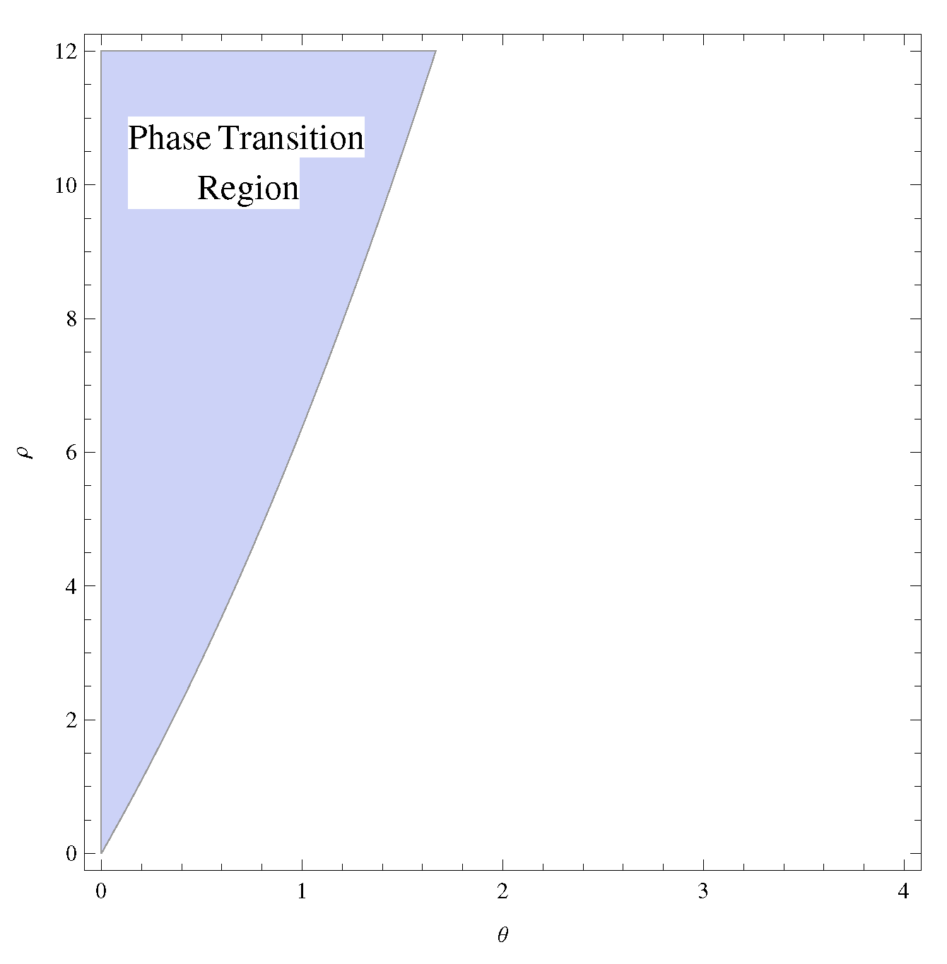
Figure 2 illustrates the blue region where
. This indicates that the cubic polynomial
has real or multiple roots within this area. Consequently, this region signifies the occurrence of a phase transition. By choosing values of
and
from this region, we can numerically demonstrate that the function
given in (
20) has three distinct fixed points.
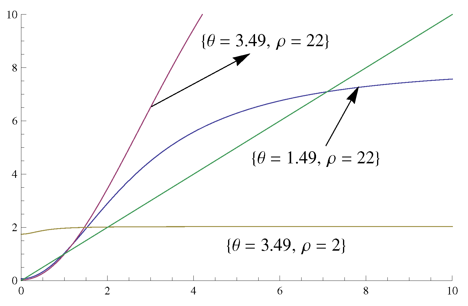
Figure 3 shows various graphs of the
function to verify the presence of a phase transition. For
and
, there are three distinct fixed points. In contrast, for
, there is only one fixed point. We know there is a one-to-one correspondence between Gibbs measures and the solutions of Equations (
10) and (11) (see [
6] for details). Thus, a phase transition is observed in the first two cases but not in the third. Therefore, we have examined the non-uniqueness of the solutions to these equations to determine if there is a phase transition in the Potts-SOS model on the second-order CT.
4. Stability Analysis of the Two-Dimensional Dynamical system
In this section, we will perform the stability analysis of the fixed points of the two-variable equation system (
18) and (19). It is known that the presence of other fixed points in the region where a fixed point is repelling (unstable) indicates the existence of multiple Gibbs measures for the corresponding Potts-SOS model, signifying a phase transition.
In stability analysis, the eigenvectors of the Jacobian matrix are crucial for assessing the stability of a fixed point [
32]. To compute the Jacobian matrix of the dynamical system given in (
18) and (19) at the point
, we first need to find the partial derivatives of
and
with respect to
t and
s. So, we compute the Jacobian matrix
J of the dynamical system given in (
18) and () as follows:
Let us calculate each partial derivative. For
, we have
Similarly, for
, we have
So, we obtain the Jacobian matrix as:
Using vector calculus of a vector-valued function of several variables, we obtain the Jacobian matrix
J given in (
22) associated with the dynamical system given in (
18) and (19) at the fixed point
as
After elementary linear algebra operations, we compute the eigenvalues of the Jacobian matrix (
23) as
These eigenvalues help determine the stability and behavior of the system near the point . As is known, in the region where the condition is satisfied, the fixed point becomes repelling (unstable). Therefore, the presence of additional fixed points in this region indicates that a phase transition occurs. Let us determine the region to which the pair that satisfies the inequality belongs.
We consider the inequality
Therefore, we analyze the following inequality:
This inequality can be broken down into two separate inequalities:
Case I:
Multiplying both sides by
, which is always positive, yields
Expanding and rearranging the terms, we obtain:
which simplifies to
Case II:
Again, multiplying both sides by
results in
Expanding and simplifying gives:
which simplifies to
Therefore, the regions in which the absolute value of the given expression is greater than 1 are characterized by the following inequalities:
These inequalities delineate the areas of interest in the
-
plane where the absolute value of the expression exceeds 1. Since inequality (
25) is a quadratic equation in
, we will solve the corresponding quadratic equation
to find the critical values of
. This will help us understand the regions where the inequality holds. So, we have
Regarding the solution set of the inequality in (), given that both and are positive, the solution set for this inequality is empty.
Now, let us proceed with the analysis of the inequality in (
25) once more. We consider the inequality:
To analyze this inequality, we perform the following steps:
Let us consider the function by
The term inside the square root is
. To ensure that the square root is real and non-negative, we require
Rewriting this quadratic expression, we get:
Solving the quadratic equation
, yields complex roots, indicating that the quadratic expression
is always positive for all real
. Hence, the square root term
is always real and non-negative.
As
: For small values of
, the expression simplifies approximately to:
As
: For large values of
, the dominant term in the expression is:
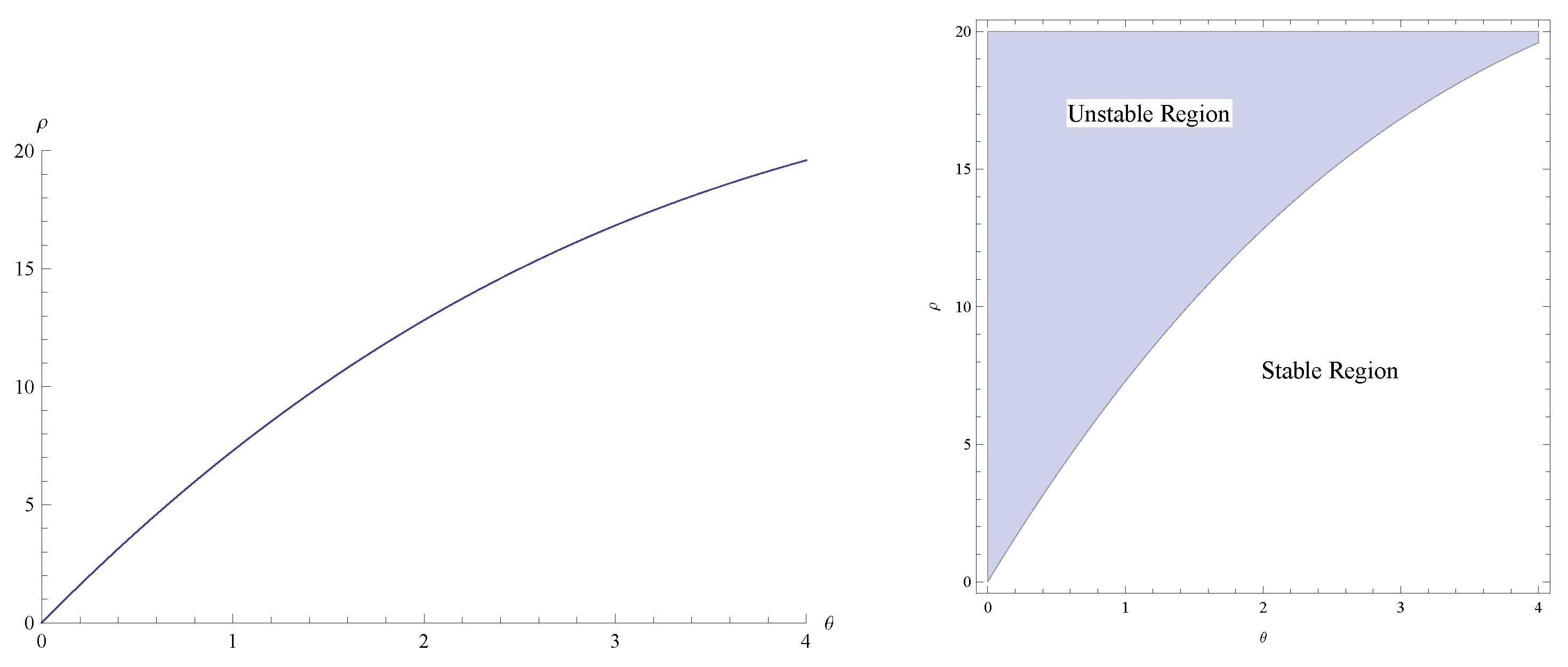
To gain a deeper understanding of the function
, we plot:
This plot illustrates how the function
varies with
and helps determine the feasible range for
(see
Figure 4(Left)). The blue area in
Figure 4(Right) illustrates the region where the inequality
is satisfied. This blue region corresponds to the domain in which the model experiences a phase transition.


