A Contrast Tree Based Approach to Two-Population Models

Preprint

Article

A Contrast Tree Based Approach to Two-Population Models

Altmetrics

Downloads

Views

Comments

A peer-reviewed article of this preprint also exists.

Matteo Lizzi^*

This version is not peer-reviewed

Submitted:

23 August 2024

Posted:

27 August 2024

You are already at the latest version

Alerts

Abstract

Building small populations mortality tables has great practical importance in actuarial applications. In recent years, several works in literature explored different methodologies to quantify and assess longevity and mortality risk, especially within the context of small populations: many models dealing with this problem usually use a two-population approach, modelling a mortality spread between a larger reference population and the population of interest, via likelihood-based techniques. To broaden the tools at actuaries’ disposal to build small population mortality tables, a general structure for a two-step two-populations model is proposed, its main element of novelty residing in a machine-learning based approach to mortality spread estimation. In order to obtain this, Contrast Trees and related Estimation Contrast Boosting techniques have been applied. A quite general machine learning-based model has then been adapted in order to generalize Italian actuarial practice in company tables estimation and implemented using data from Human Mortality Database. Finally, results from the ML-based model have been compared to those obtained from the traditional model.

Keywords:

Subject: Business, Economics and Management - Econometrics and Statistics

1. Introduction

Producing accurate mortality projections is often of great importance in an actuarial context, in order to predict death rates for pricing or reserving purposes, to construct policyholders’ death tables for an insurance company, or, more generally, to accurately assess the mortality of a population of interest such as the participants of a pension fund. While mortality projection has received a considerable amount of attention in actuarial literature, the main focus usually involves national or similarly-sized populations: small populations, such as those of regions within a country or groups of annuitants, are far less studied.

Quantifying and projecting mortality for such small populations is non-trivial, because their mortality rates tend to be characterized by high variability and irregular behaviour, scarce availability of data in temporal terms and missing records. Furthermore, due to the usually short-period availability of data, mortality projections are quite uncertain and sensitive to the choice of fitting time period: plain extrapolation of historic trends could produce questionable results and biologically implausible death tables. In such cases, standard mortality models may not be relevant and the resulting mortality rates could be unreliable. Consequently, using established models, such as the Lee-Carter model ([1]), to project mortality for small populations is not advisable ([2,3]), as it could lead to unrealistic results. Furthermore, population size can have a noticeable effect on the variation of parameters’ estimates, as in the case of Cairns-Blake-Dowd model ([4,5]). Moreover, as observed by [6], the aim of mortality projection models should be twofold: on one hand the predictions produced by the models have to be accurate, as usual in actuarial literature; on the other hand the models’ output should be stable in respect to annual updates of the data. This is to ensure that decision makers, such as annuity providers or pension authorities, do not suffer consequences (respectively, significant shifts in liabilities and capital requirements or fluctuations in statutory retirement age) from result volatility or systematic errors. Stability requirements are particularly difficult to meet for smaller populations. Nonetheless, small populations’ mortality models have great practical interest, for example in evaluating undertaking-specific mortality tables relative to a portfolio of contracts or in tackling issues pertaining to longevity swaps in the context of pension scheme de-risking.

To overcome such difficulties in modelling mortality for small populations, the mortality parameter estimation is performed in reference to the mortality profile of some larger group, economically and socially similar to the population of interest: borrowing information in such a way could lead to more stable results, as noted by [7]. This approach to the problem is known as two-population modeling and can lead used to the definition of several callses of models, from extensions of Lee-Carter model (see, e.g., [8,9]) and Cairns-Blake-Dowd (as in [10]) model to Bayesian approaches ([11]) and frailty-based methods ([3]). More extensive reviews are available in [12,13].

Borrowing terminology and model specification from [13], the larger population will be denoted as reference population and the smaller population of interest as book population. Two-population models can be written using a general formulation in terms of central mortality rates

m_{x t}

, respectively for reference and book populations, as:

\begin{matrix} D_{x t}^{R} \sim Pois (E_{x t}^{R} m_{x t}^{R}); & log m_{x t}^{R} = α_{x}^{R} + \sum_{j = 1}^{N} β_{x}^{(j, R)} κ_{t}^{(j, R)} + γ_{t - x}^{R} \end{matrix}

(1)

\begin{matrix} D_{x t}^{B} \sim Pois (E_{x t}^{B} m_{x t}^{B}); & log m_{x t}^{B} - log m_{x t}^{R} = α_{x}^{B} + \sum_{j = 1}^{M} β_{x}^{(j, B)} κ_{t}^{(j, B)} + γ_{t - x}^{B} \end{matrix}

(2)

Note that, in Equation (2), book population modeling is expressed in terms of the difference between reference and book population mortality: the mortality of book population is not directly modelled: rather the mortality spread between reference and book population is. Therefore, quantities in Equation (2) refer to mortality trend differences, so that book population average mortality level is

α_{x}^{R} + α_{x}^{B}

and cohort effect is

γ_{t - x}^{R} + γ_{t - x}^{B}

. Depending on how the models are specified, additional constraints may be needed in order to ensure uniqueness of parameter estimation for Equations (1) and (2). The parameter estimation is performed using maximum likelihood in two steps: firstly relative to the reference population and then, conditional on the first-stage estimation, the parameters describing mortality spread between the two populations are estimated in a second stage. Such approach, widespread in actuarial literature for small population models (see, e.g., [3,10,12,14]), is based on the assumption that mortality rate differences can be modeled in the same way as mortality rates are, using the same functional form as in [15].

Mortality projection is then performed by specifying the dynamics of period indexes, which are modelled using a multivariate random walk with drift. As for the book populations, it is assumed that in the long run the two populations will experience similar mortality improvements, thus the spread in time indexes and cohorts effects are modelled as stationary processes (see [13] for more details). Two-step estimation for two population models then relies on the distributional assumptions for number of deaths in reference and book populations and on likelihood based estimation for modelling mortality spread.

The purpose of this paper is to present a two-population model where mortality spread is estimated using machine learning techniques, namely Contrast Trees and Estimation Contrast Boosting proposed by [16]. The model is first described in general terms and then adapted do generalize Italian actuarial practices for company table estimation. Using data from Human Mortality Database, this new model is evaluated for some book populations and then compared to traditional methodology.

The remainder of this work is organized as follows: in Section 2, Contrast Trees terminology and algorithms are briefly recalled (Section 2.1), then the Italian actuarial practice for company table estimation is described and extended making use of Contrast-Tree related techniques (Section 2.2). Some preliminary consideration about the data are reported in Section 2.3. Section 3 presents and discusses the results from the extended model, firstly by addressing some issues about model calibration (Section 3.1) then assessing the performance of the extended model using the traditional one as a benchmark (Section 3.2); finally, in Section 4, some conclusions are drawn.

2. Materials and Methods

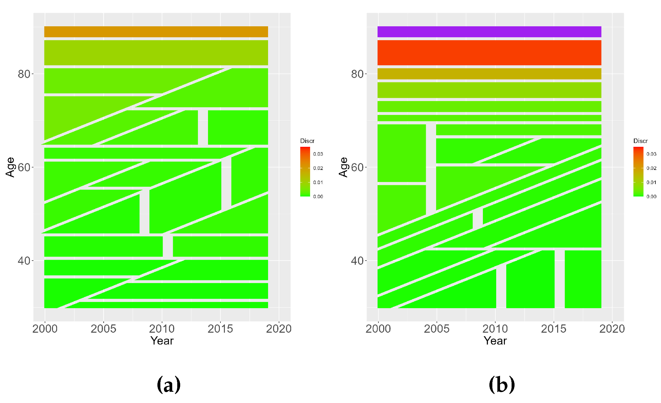
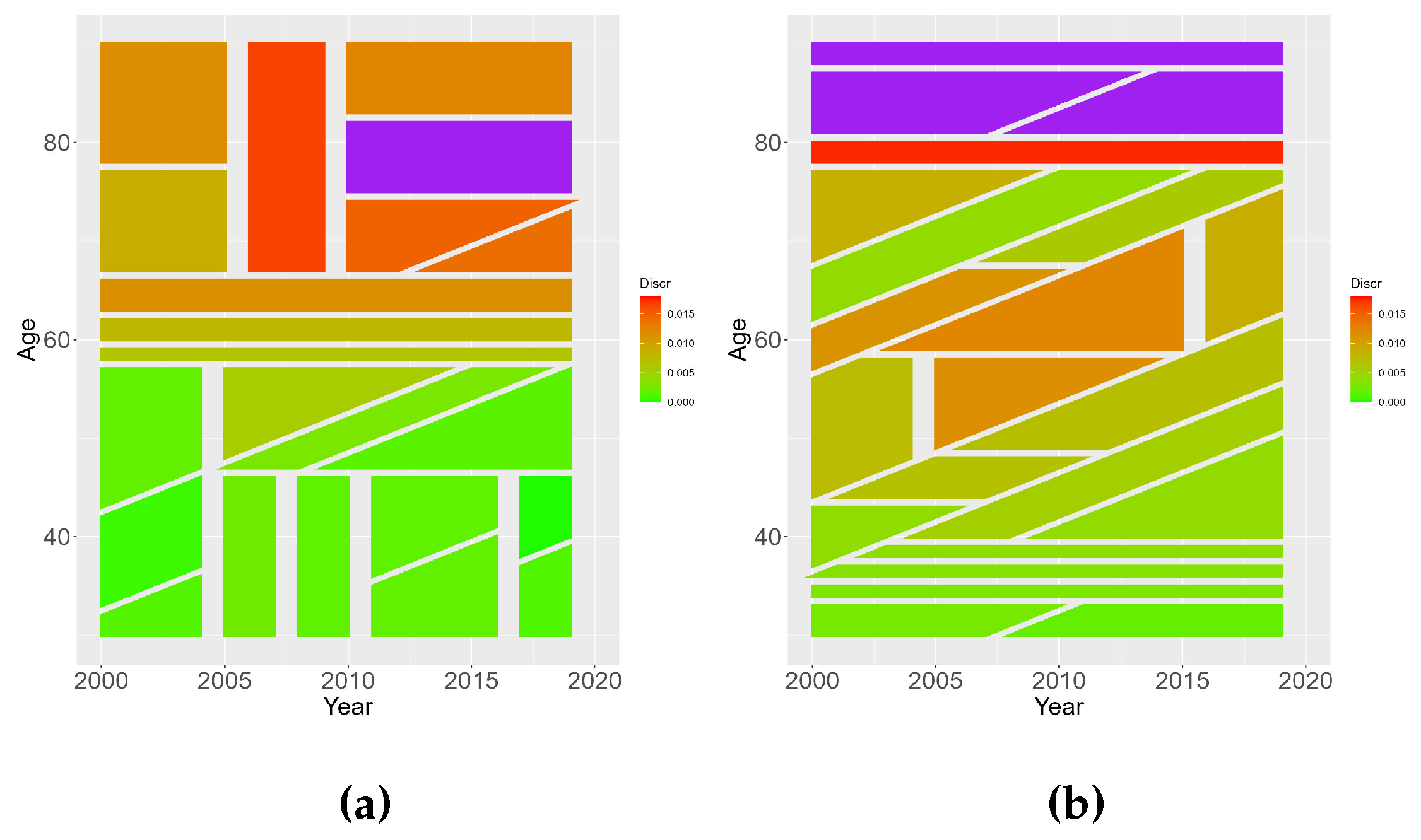
2.1. Contrast Trees and Estimation Boosting

Contrast Trees (CT) are a general methodology that, leveraging tree-based machine learning techniques, allows for assessing differences between two output variables defined on the same input space, be them predictions resulting from different models models or observed outcome data. Specifically, the goal of the Contrast Trees method is to partition the input space to uncover regions presenting higher values of some difference-related quantity between two arbitrary outcome variables ([16]). Moreover, a boosting procedure making use of CTs can be constructed, in order to reduce differences between the two target variables once differences have been uncovered.

Available data consist of N observations of the form

{x_{i}, y_{i}, z_{i}}_{i = 1}^{N}

, where

x_{i}

is a P-dimensional vector of observed numerical predictor variables and

y_{i}

and

z_{i}

are the corresponding values of two outcome variables. These can be estimates for a given quantity from different models, or the observed values of a certain quantity of interest. Given a certain sub-region

X^{*}

of the input space, a discrepancy measure, describing the difference between the outcome variables, is defined as a function of the data points in the sub-region as follows:

d = D ({y_{i}}_{x_{i} \in X^{*}}, {z_{i}}_{x_{i} \in X^{*}})

(3)

The particular choice of discrepancy function depends on the problem at hand. While discrepancies are conceptually similar to loss functions, it must be noted that in the context of Contrast Trees, they are not required to be convex, differentiable nor expressible as sum of terms, each involving a single observation. In the following, we’ll make use of the mean absolute difference discrepancy :

d_{m}^{[1]} = \frac{1}{N_{m}} \sum_{x_{i} \in R_{m}} | y_{i} - z_{i} |

(4)

where

N_{m}

is the number of data points (or, alternatively the sum of weights) relative to region

R_{m}

. A quick review of possible choices for discrepancy functions, and their relation to different estimation problems, can be found in [16].

Contrast Trees produce a partition of the input space into M components, each one with an associated value for discrepancy. Such partition can be analyzed to assess discrepancy patterns, bearing some similarities to residuals analysis in Generalized Linear Models framework. A brief overview of the iterative splitting procedure of the input space is given in Algorithm 1.

Algorithm 1 Iterative splitting procedure - Construction of a Contrast Tree
Require: ${x_{i}, y_{i}, z_{i}}_{i = 1}^{N}$
⋄ Choose $M^{*} \in N$	▹ Maximum number of regions
⋄ Choose $n^{*} \in N$	▹ Minimum number of data points in a region
for $1 \leq M \leq M^{*}$ do	▹ Loop over successive trees
⋄ The input space is partitioned into M disjoint regions ${R_{m}}_{m = 1}^{M}$ ;
for $1 \leq m \leq M$ do	▹ Loop over regions in a tree
for $1 \leq j \leq P$ do	▹ Loop over predictors
for all $x_{j}$ do	▹ Loop over values of a predictor
⋄ Define two provisional sub-regions $R_{m}^{(l)}$ and $R_{m}^{(r)}$ , with corresponding discrepancies $d_{m}^{(l)}$ and $d_{r}^{(l)}$ : $x \in R_{m} x_{j} \leq s \to R_{m}^{(l)}; x \in R_{m} x_{j} \geq s \to R_{m}^{(r)}$ This rule is the same as for ordinary regression trees for numeric variables (see [17] for further details);
⋄ Calculate the quality of the split $Q_{m} (l, r)$ : $Q_{m} (l, r) = (f_{m}^{(l)} \cdot f_{m}^{(r)}) max {(d_{m}^{(l)} d_{m}^{(r)})}^{β}$ where $f_{m}^{(l)}$ and $f_{m}^{(r)}$ are the quota of observations in region $R_{m}$ falling within each provisional sub-region and $β$ is a regulation parameters: as found by [16], results are insensitive to its value;
end for
end for
⋄ The split point $s^{}$ for variable $x_{j^{}}$ , whose value maximizes $Q_{m} (l, r)$ , with associated discrepancies $d_{m}^{* (l)}$ and $d_{m}^{* (r)}$ is associated to the m-th region;
⋄ Calculate discrepancy improvement for the m-th region: $I_{m} = max (d_{m}^{* (l)}; d_{m}^{* (r)}) - d_{m}$
if $I_{m} < 0 \forall m$ then
	▹ Stopping condition (1)
⋄ STOP
end if
end for
⋄ The region $R_{m}^{*}$ , whose associated split maximizes $I_{m}$ , is replaced by its associated sub-regions, s.t. the input space is now partitioned into $M + 1$ regions
if $# (R_{m}) \leq n^{} \forall m$ then*	▹ Stopping condition (2)
⋄ STOP
end if
end for

Results from the CT procedure can be summarized in a so-called lack-of-fit (LOF) curve, which associates to the m-th region the following coordinates:

{[\frac{1}{N} \sum_{d_{j} \geq d_{m}} N_{j}; \frac{\sum_{d_{j} \geq d_{m}} d_{j} N_{j}}{\sum_{d_{j} \geq d_{m}} N_{j}}]}_{m = 1}^{M}

(5)

Where the abscissa is the quota of data points having discrepancy grater or equal to that of the m-th region and the ordinate is the average weighted discrepancy in those same regions. Contrast Trees can be applied to assess the goodness-of-fit of a certain model, by choosing as output variables (i.e., "contrasting") predicted values from the model and observed ones. High-discrepancy regions resulting from the procedure can be easily detected and interpreted, without having to formulate distributional hypotheses to define a likelihood: multiple models, of any nature, can be compared estimating a Contrast Tree for each one, contrasting predicted values with out-of-sample observed outcomes. An application of CTs to model diagnostics in the context of mortality models can be found in [18] .

Contrast Trees may also be employed to improve model accuracy, by means of an iterative procedure that reduces uncovered errors and calculates an additive correction to produce more accurate predictions. Estimation Contrast Boosting (ECB) gradually modifies a starting value of z using an additive term, reducing its discrepancy with y, producing, at each step k, a partition of the input space where every element m has an associated update

δ_{m}^{(k)}

. The resulting prediction for z is then adjusted accordingly, so that an updated estimate

\hat{z} (x)

is produced.

Please note that in Estimation Contrast Boosting, the two response variables are no longer equivalent: response y is taken as the reference, while response z is adjusted. A quick presentation of the boosting procedure is given in Algorithm 2. Since any point

x

in the input space lies within a single region

R_{m}^{(k)}

of each of the trees resulting from the ECB procedure, each with associated updates

δ_{m}^{(k)}

, and given an initial value

z (x)

, the boosted estimate

\hat{z} (x)

is computed as:

\hat{z} (x) = z (x) + \sum_{k = 1}^{K} δ_{m}^{(k)}

(6)

More detail about the iterative splitting procedure to produce Contrast Trees or about ECB algorithm can be found in [16,18].

Algorithm 2 Estimation Contrast Boosting

Require:

{x_{i}, y_{i}, z_{i}}_{i = 1}^{N}

⋄ Choose maximum number of iterations K;

⋄ Choose maximum number of regions M for each iteration;

for

1 \leq k \leq K

⋄ Build a Contrast Tree of

z^{(k - 1)}

versus y using discrepancy in Equation (4), with

z^{(0)} = z

, thus partitioning input space in M regions

R_{m}^{(k)}

;

⋄ Update

z^{(k - 1)}

as follows:

z^{(k)} \leftarrow z^{(k - 1)} + α δ_{m}^{(k)} x \in R_{m}^{(k)}

Where

0 < α \leq 1

is a learning parameter and the update

δ_{m}^{(k)}

is found by imposing

D ({y_{i}}_{x_{i} \in R_{m}^{(k)}}, {z_{i}^{(k)}}_{x_{i} \in R_{m}^{(k)}}) = 0

;

end for

2.2. Small Population Tables in Relation to Italian Actuarial Practice

In Italian actuarial practice, the assessment of mortality in life insurance companies is heavily influenced from ISVAP Regulation N.22 of 4th April 2008 and its successive modifications1. Article 23-bis, comma 9 of the regulation states that "The Insurance company conducting life business presents to IVASS the comparison between technical bases, different from interest rates, used for the calculation of technical provisions, and the results of direct experience". This happens trough the filling of table 1/1 of Module 41 contained in the Additional Informations to Financial Statements ("Informazioni aggiuntive al bilancio d’esercizio").

The module is organized separately by risk type (longevity or mortality), product type, age range and sex: these features define the risk classes to be considered. The underlying idea, common in actuarial mathematics, is to analyze the portfolio separately for groups defined by known risk factors, so that individuals composing these groups can be considered homogeneous from the point of view of probabilistic evaluation. The comparison between direct experience and technical bases consists in reporting the expected number of deaths in the company portfolio, the expected sum of benefit to be paid, the actual number of deaths and the actual paid sum of benefits. Expected number of deaths

{\tilde{d}}_{x}^{C}

and expected sum of benefit to be paid

{\tilde{B}}_{x}^{C}

are defined as follows:

{\tilde{d}}_{x}^{C} = q_{x}^{(1)} * n_{x}^{C} {\tilde{B}}_{x}^{C} = q_{x}^{(1)} * S_{x}^{C}

where

n_{x}^{C}

is the number of insureds of age x in risk cluster C at the beginning of the year,

S_{x}^{C}

is the total insured sum for insureds of age x in cluster C at the beginning of the year and

q_{x}^{(1)}

is the probability of death between ages x and

x + 1

, usually dependent on sex. The table

{q_{x}^{(1)}}_{0}^{ω}

constitutes part of the prudential technical basis used for pricing purposes. The time period to which all quantities refer is the solar year of the Financial Statements in consideration.

While not required by Solvency II directive, in Italian actuarial practice a very similar approach is adopted in order to produce the mortality hypotheses to be used in the calculation of best estimate liabilities and, more generally, to estimate company mortality tables, especially in the case of products subject to mortality risks. In this case, given a certain risk cluster C usually described by sex, risk type (mortality, longevity) and product type (e.g., endowment or term life insurance), an adaptation coefficient

α^{C}

is calculated as:

α_{d}^{C} = \frac{\sum_{x} d_{x}^{C}}{\sum_{x} q_{x}^{(2)} n_{x}^{C}}

(7)

or, using the sum of benefits as a reference:

α_{B}^{C} = \frac{\sum_{x} B_{x}^{C}}{\sum_{x} q_{x}^{(2)} S_{x}^{C}}

(8)

where

d_{x}^{C}

is the observed number of deaths for age x in cluster C,

B_{x}^{C}

is the sum of benefits paid for insureds dead at age x in cluster C and

q_{x}^{(2)}

is the probability of death, distinct by sex, from some reference mortality table, usually a national table of some sort (e.g., SIM2011 table or ISTAT table for people residing in Italy). The table

{q_{x}^{(2)}}_{0}^{ω}

is a demographic realistic technical base that can be updated over time.

The adapted death rates

q_{d, x}^{C}

q_{B, x}^{C}

which will constitute the company death tables are then calculated as follows:

q_{d, x}^{C} = α_{d}^{C} q_{x}^{(2)} q_{B, x}^{C} = α_{B}^{C} q_{x}^{(2)}

(9)

Essentially, this method scales one-year death probabilities in order to reproduce the total number of deaths or the total benefits paid. Data used for the calculation include observations from the last available calendar years. Usually, ten calendar years of data are used: this ensures a sufficiently stable output without having to resort to data from much earlier calendar years, which is often not available and could not reflect the actual, more recent, trends in mortality dynamics. This methodology features ease of implementation, but applies the same adaptation coefficient to all age classes, thus creating a mortality profile which has the same shape as the reference one, while the company underwriting process may affect each age group differently. In the remainder of this work, we will refer to this technique as "table scaling".

To overcome the limitations of table scaling, the ECB algorithm briefly described in Section 2.1 can be utilized to build mortality tables for small populations, using a machine learning approach for mortality spread calculation and generalising the Italian actuarial practice. At the best of the author’s knowledge, this is the first attempt in applying a machine learning approach to compute mortality spread in a two-population model.

Let

Q_{X, t}^{R}

and

Q_{X, t}^{B}

be some quantity describing mortality in terms of predictor matrix X and calendar year t respectively for reference and book populations, available for observation years

1, \dots, T

. These can be one-year death probabilities, central mortality rates, mortality odds or, more generally, any quantity describing mortality in a population. The Estimation Boosting algorithm can then be applied to variables

Q_{X, t}^{R}

and

Q_{X, t}^{B}

, using the quantity relative to reference population as the z input of Algorithm 2. The ECB procedure then estimates updates

δ_{X, (1, \dots, T)}^{(k)}

, that can be used to transform the quantity

Q_{X, t}^{R}

relative to reference population into the corresponding quantity relative to book population, as per Equation (6):

{\hat{Q}}_{X, t}^{B} = Q_{X, t}^{R} + \sum_{k = 1}^{K} δ_{X, (1, \dots, T)}^{(k)}, t = 1, \dots, T

A shift in the target of the estimation boosting procedure must be emphasized : while in [16] the goal was to reduce differences between outcomes y and z by producing an updated estimate

\hat{z}

and calculate the updates

δ_{m}^{(k)}

only as a consequence, now the objective is to obtain the updates themselves, in order to transform the quantity of interest of the reference population into that of the book population. Also note, on the terminological side, that the word "reference" is used in two different meanings in the context, respectively, of two-population models and Estimation Contrast Boosting: in the first case it indicates to the larger population, whose mortality is used as a baseline for mortality spread modelling. In the second case, it designates the y output variable of the ECB algorithm, in this case

Q_{X, t}^{B}

, which in the present application is relative to the book population.

Now, the quantity

Q_{X, t}^{R}

can be projected to calendar years

T + 1, \dots

using some standard mortality projection model, which is feasible for the reference population, thus obtaining estimates

{\tilde{Q}}_{X, t}^{R}

for the quantity of interest in future calendar years. Some assumptions on the updates

δ_{X, (1, \dots, T)}^{(k)}

must then be made, to extend their range of application from calendar years

1, \dots, T

, on which they have been estimated, to projection calendar years

T + 1, \dots

. The extended updates

δ_{X, (T + 1, \dots)}^{(k)}

can then be applied to projected estimates in order to obtain boosted estimates

{\hat{Q}}_{X, t}^{B}

for the book population relative to projection calendar years:

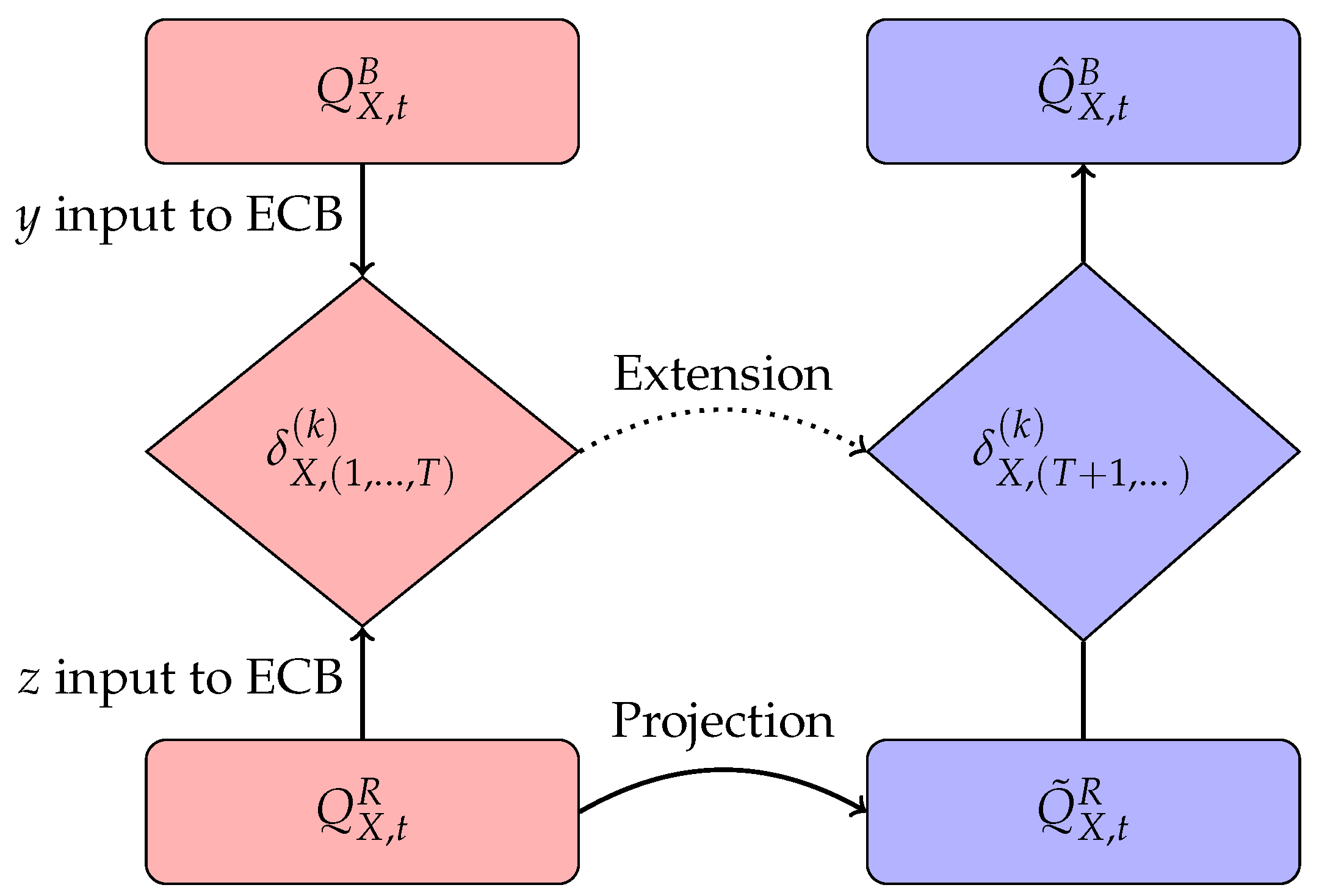
{\hat{Q}}_{X, t}^{B} = {\tilde{Q}}_{X, t}^{R} + \sum_{k = 1}^{K} δ_{X, (T + 1, \dots)}^{(k)}, t = T + 1, \dots

This methodology pertains to two-step models for small population, with the main difference residing in the quantification of mortality spread, which now relies on a machine-learning technique. It must be emphasized that the book population is not requested to be similar to the reference population in terms of geographical, historical or socio-economical features. In such cases, however, a faster estimation boosting convergence and, more generally, a better model performance can be expected. The procedure just described is summarized in Figure 1, and, in the remainder of this work, we will be referred to as "ECB adaptation".

Before model implementation, some critical issues must be pointed out. First of all, no mechanism for the extension of updates to projection calendar years is straightforwardly provided. So, not having at disposal a tool for update projection, a reduced form of the input design matrix for Estimation Contrast Boosting could be used, adopting as predictors just variables age, cohort, or a combination of the two: this issue will be further addressed in Section 3.1. Also note that using data from the same calendar years for reference population mortality projection and ECB calibration is not strictly necessary: it could be possible to use a longer time series of data for mortality projection, while making use a shorter time series to calibrate the ECB updates. In fact, not using a mechanism to project the ECB updates means to implicitly assume the the updates themselves, i.e., the transformation function from reference population to book population mortality, do not change with time. This means assuming that relative mortality levels are stable during both ECB calibration and projection time periods, thus suggesting the use of data relative to most recent years.

Aside from these points of attention, this model is quite flexible, leaving considerable freedom in the choice of the quantity of interest, the projection model and the structure of the design matrix used as input in the ECB updates’ estimation.

2.3. Data

HMDHMD

Data used for numerical evaluation have been provided by the Human Mortality Database [19]. Due to lack of company-specific data, Italian male population has been considered as reference population, while Austria, Slovenia and Lithuania males are considered as book populations. The time period taken into consideration is 1950-2019, for ages comprised between 30 and 90. Calendar years from 2000 to 2019 will be used for mortality projection purposes. Data relative to Slovenia and Lithuania are available, respectively, starting from 1983 and 1959. The first two populations can be considered close, at least in geographical terms, to the reference population. On the contrary, the Lithuanian population has been selected in order to investigate the ECB adaptation procedure behaviour when book and reference populations differ substantially.

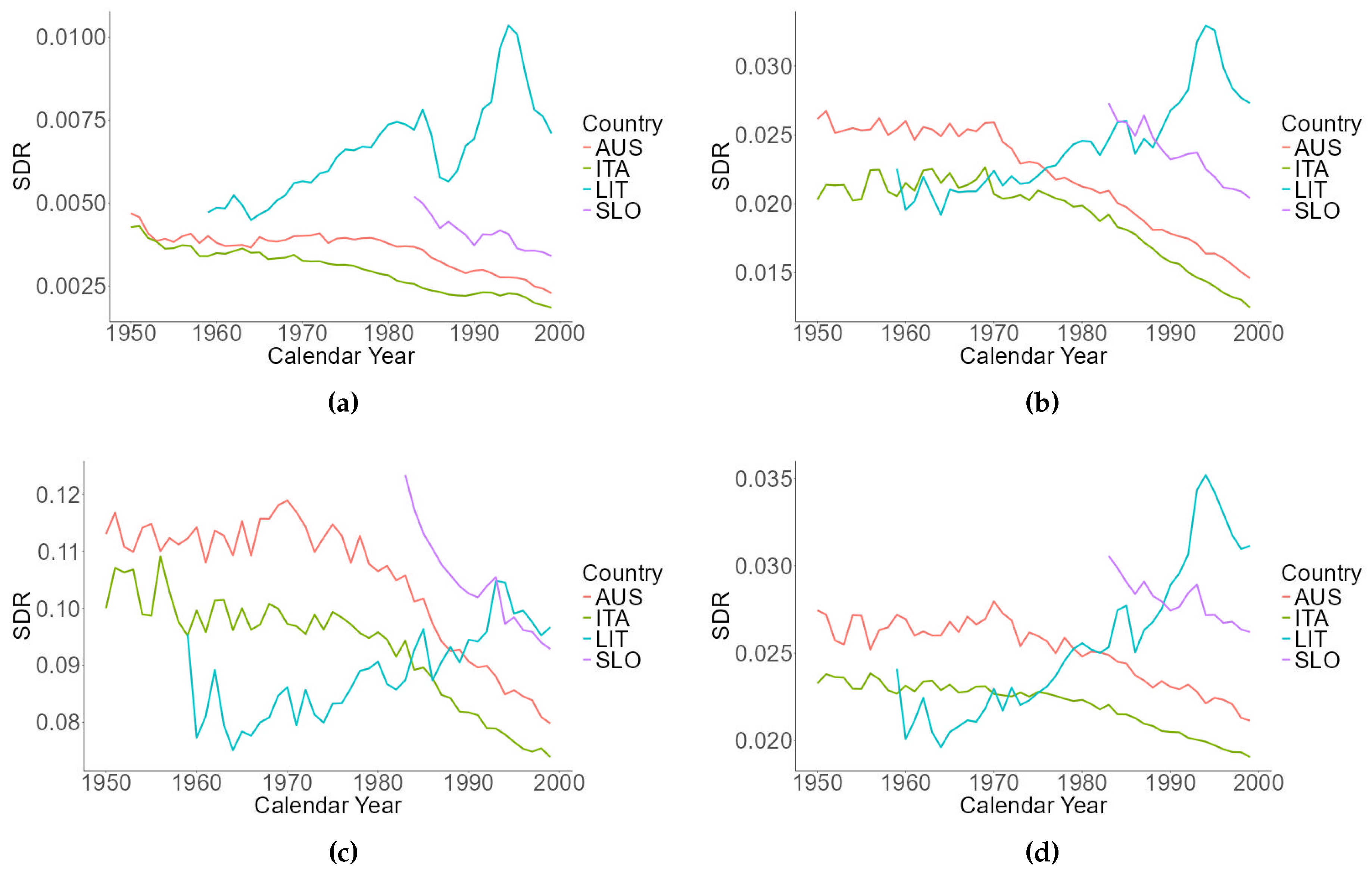
Using the approach proposed by [20], to have a first qualitative evaluation of similarity between two reference and book populations, Standardized Death Rates (SDR) relative to period 1950-1999 are calculated, separately for age groups 30-50, 50-70, 70-90, and then for the whole age range in consideration. Relative to country I, ages ranging from

a_{s}

a_{e}

, using reference population R, SDRs are computed as:

{SDR}_{t, a_{s}, a_{e}}^{I} = \frac{\sum_{x = a_{s}}^{a_{e}} E_{x, t}^{R} m_{x, t}^{I}}{\sum_{x = a_{s}}^{a_{e}} E_{x, t}^{R}}

where m denotes the central death rate and E the central exposure-to-risk. Results are reported in Figure 2.

Italian and Austrian mortality present a similar trend, with quite a regular behaviour, both on separate and joint age groups. Slovenian mortality data, while available only since 1983, displays a similar, albeit more irregular, pattern. This is expected since Slovenian population is the least numerous of the three countries. On the other hand, Lithuanian mortality exhibits a completely different pattern, being smaller than the Italian one until year 1975, then steadily increasing until year 1995 and eventually decreasing again.

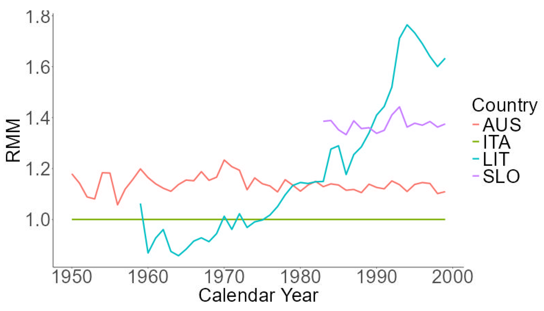
Following [12], a relative Measure of Mortality (RMM) il aslo computed as:

{RMM}_{t, a_{s}, a_{e}}^{I} = \frac{\sum_{x = a_{s}}^{a_{e}} E_{x, t}^{R} m_{x, t}^{I}}{\sum_{x = a_{s}}^{a_{e}} E_{x, t}^{R} m_{x, t}^{R}}

The nearer RRM value is to 1, the closer the book and reference population are on average in terms of mortality. As it can be seen from Figure 3, the mortality of reference population tends to be the lowest, in contrast to what would presumably happen using, say, a group of annuitants as book population.

Again, we can clearly see that Italian, Austrian and Slovenian mortality evolve similarly. Lithuanian relative mortality dynamics behaves differently: while initially lower in respect to reference population, it gets higher and higher from the mid-sixties to the mid-nineties, then decreases. This suggests caution in the choice of the time frame per ECB mortality boosting calibration.

3. Results

3.1. Model Calibration

Since the focus of this paper is not the choice of the best mortality model for the reference population, but rather studying the implementation of a machine learning-based mortality spread estimation technique, the choice of the mortality model for reference population mortality projection has not been investigated in detail. Projection has been performed using a simple Lee-Carter mortality model, with temporal indexes dynamics described by a random walk with drift, as suggested by [21]. Lee-Carter dynamic mortality model has been implemented using the R package "StMoMo" [15]. The time period for calibrating mortality projection for the reference population is chosen to be from 1950 to 1999, using ages from 30 to 90. Central mortality rates, with corresponding death rates, have been projected to period 2000-2019. Central mortality rates resulting from Lee-Carter projection can be transformed into one-year death probabilities using the constant force of mortality hypothesis (see, e.g., [22]):

q_{x, t} = 1 - e^{m_{x, t}}

Contrast Trees and Estimation Contrast Boosting have been evaluated using the R package "ConTree" developed by [23], using as response variable one-year death probabilities.

As stated before, the time frame used for ECB adaptation calibration does not have to coincide with the one used for reference population mortality projection. To investigate which time period should be used to estimate ECB updates, different Contrast Estimation Boosting adaptations are performed for different starting years, from 1965 and every fifth year until 1999. For Slovenia, data allows for year 1983 as minimum starting date. Each ECB procedure was performed, for the sake of simplicity, using only Age as predictor (more on that in the following) and adopting central death rates as quantity of interest, s.t.

Q_{X, t}^{P} = m_{x, t}^{P}

: the updates resulting from each procedure were applied to Italian projected mortality rates, obtaining an estimate for book population mortality rates. A Contrast Tree has been estimated using discrepancy 4 for each ECB output. Data relative to the 2000-2019 time frame is split in half into training and test set for Contrast-Tree estimation and evaluation purposes, respectively, using maximum dissimilarity approach ([24]): corresponding lack-of-fit curves are reported in Figure 4.

Very different behaviours are apparent from the first and third panel: while for Austrian book population using a longer data series leads to more accurate estimation of future book population mortality rates, for Lithuanian population the situation is reversed. Moreover, relative variation in average discrepancy for Lithuanian book population (as can be seen in the far right of the graph) is quite impacted from the choice of starting year. Such behaviour can be explained in terms of Relative Mortality Measures reported in Figure 3: Austrian mortality dynamics is quite aligned with the Italian one, so using a longer data series allows for a more robust estimation of ECB updates, which do not presumably change too much in the period 1965-1999 (please note that calendar years 1950-1964, where Austrian mortality exhibits greater volatility in relative mortality, were not used in ECB estimation). On the other hand, Lithuanian relative mortality evolves significantly in the 1959-1999 time period and the assumption of time independent ECB updates should be called into question. Results for Slovenian book population constitute a middle ground: ECB updates produced using data from just 1990 onwards yield worse results in comparison to 1980, across all input space. This suggests that, due to the irregularity of Slovenian mortality pattern, using only the more recent calendar years to estimate the updates could lead to unreliable results.

In order to assess the most sensible choice for ECB predictors and given the absence of an obvious choice for a projection mechanism for the updates

δ

, it should be observed that using only variables age and cohort from ECB modelling does not require any form of time series extrapolation, as already stated by [25]. Therefore, for each book population, three ECB adaptations were performed, using as predictors variables Age, Cohort, or both. As before, the quantity of interest is the central mortality rate. The updates have been calibrated, for each book population, on the minimum discrepancy time interval identified previously. The resulting mortality rates for book populations have been compared to the observed ones using lack-of-fit curves, average discrepancy, Root Mean Square Error (RMSE) and Mean Absolute Percentage Error (MAPE). Data for Contrast Tree estimation have been split into training and test set using maximum dissimilarity approach, while RMSE and MAPE have been calculated on the whole projection period. Results are shown in Figure 5 and in Table 1.

For all three book populations similar conclusions can be drawn: cohort ECB features the highest discrepancy across all input space. For Slovenian and Austrian population, Age-Cohort ECB produces the best performances in high discrepancy regions, but when considering the entirety of the input space, Age-based ECB seems to perform slightly better. As for Lithuanian book population, Age ECB seems to consistently produce more accurate outputs. Note the different scale on ordinate axis for Lithuanian discrepancy. Performance statistics reported in Table 1 are consistent with conclusions from the LOF curves: with the exception of RMSE for Cohort ECB for Slovenian and Lithuanian book populations, Age-based Estimation Contrast Boosting seems to consistently yield better performances.

3.2. Generalization of Italian Actuarial Practice Using ECB Adaptation

The procedure presented in Section 2.2 has been further specified and adapted, in order to build a generalized machine-learning version of the table scaling technique. To mimic the procedure, one-year death probabilities

q_{x, t}

have been adopted as quantity of interest. Because of the additive nature of the updates and to replicate the multiplicative scaling used to adapt national mortality tables, Estimation Contrast Boosting has been applied to the natural logarithm of such probabilities. The updates

δ_{X, (1, \dots, T)}^{(k)}

have been estimated using data relative to time period 1990-1999, notwithstanding the results in Section 3.1, to reproduce the length of the time series usually available to an insurance company. The ECB updates have been extended to calendar years 2000-2019 using Age-based Estimation Contrast Boosting.

Performances have been assessed comparing adapted death probabilities for the book population, observed death probabilities and rescaled death probabilities, by means of Contrast Trees with discrepancy 4, RMSE and MAPE. Data used to estimate and evaluate Contrast Trees are split in half using maximum dissimilarity approach, while RMSE and MAPE have been calculated on the whole projection period.

Lack-of-fit curves relative to the three book populations are reported in Figure 6. In all three cases, the discrepancy resulting for the ECB boosting procedure is lower than the one resulting from mortality scaling across the whole input space. However, the scale of discrepancy is quite different across the book populations. LOF curve for ECB procedure presents a flatter profile, while, for mortality scaling LOF, curve presents very high values of discrepancy in the left regions: this means that accuracy issues relative to mortality scaling occur especially in high discrepancy regions. There, the flexibility of ECB procedure allows for separate updates for different age classes. While it is possible to extend mortality adaptation by estimating different coefficients on different age classes, in the case of ECB such classes are determined directly from the procedure and do not require further input, nor expert judgement. It should also be recalled that the assumption of relative mortality stability between reference and book population is not verified for Lithuania: so results relative to Lithuanian book population must be taken with caution.

Numerical indicators in Table 2 indications are coherent with LOF curves, although they provide less detail: ECB adaptation features lower average discrepancy and RMSE in all three cases, while MAPE is comparable for Austrian and Slovenian book population. It can be noted, in line with Figure 6, that Austrian book population is characterized by the lowest values of the inaccuracy indexes, followed by Slovenia and then Lithuania.

As already observed, model performances differ most in high-discrepancy regions. Since the input space used in Contrast Tree estimation is quite simple, consisting only of age, calendar year and cohort predictors, we can represent the pattern of discrepancy on the input space for ages 30-90 and calendar years 2000-2019, easily identifying such regions. Results are presented in Figure 7, Figure 8 and Figure 9 for Austrian, Slovenian and Lithuanian book populations, respectively: regions filled in green have lower discrepancy values, while red ones have higher discrepancies. For the sake of image readability, regions whose associated discrepancy value exceeds the maximum on right-side scale are filled in purple.

For Austrian males, both models are quite well-behaved (i.e., produce relatively low values for discrepancy) until age 65. For older ages, the accuracy of both models starts to deteriorate, but this effect is much more noticeable for table scaling and particularly sizeable at very old ages, regardless of calendar year. For Lithuanian book population this pattern is much less evident, and discrepancy is more evenly distributed in the input space. The better performances for ECB adaptation are apparent across all input space.

Similar considerations can be applied to Slovenian male population. Please note that the almost constant value of discrepancy on input space corresponds directly with the flat profiles of LOF curves reported in panel (b) of Figure 6.

For Lithuanian book population the pattern described for Austria and Slovenia is less evident. Although high discrepancy tends to be more evenly distributed in input space, older age regions still tend to be associated with worse model performances.

4. Discussion

In this paper, using the tools provided by Contrast Trees, a Machine Learning approach to mortality spread estimation in the context of two-population models has been constructed. The proposed model computes mortality spread using Estimation Contrast Boosting (ECB), and produces book population mortality table by applying ECB updates to the mortality-related quantities of a reference, much larger, population, whose mortality can be projected using well-attested models. This ECB-based model provides a good degree of flexibility, allowing for a variety of mortality-related quantities of interest, dynamic mortality models for reference population projection and predictor structure for ECB updates estimation. While some caution is advised when assessing the relative mortality structure of the two populations taken into account and when extending the ECB updates to mortality projection time frame, the model can be quite easily implemented.

Finally, taking into account Italian actuarial practice, ECB mortality adaptation has been used to generalize the mortality scaling usually used within insurance companies for estimating a realistic demographic technical basis. The new procedure leads to more accurate estimation results compared to those obtained with the traditional technique and also allows to overcome its main limitation of applying the same adaptation coefficient to all ages. While these results seems promising, further investigation is needed since the ECB methodology has not been tested on company data, whose Relative Mortality Measure could behave differently in respect to the results in Section 2.3.

Funding

This research received no external funding.

Data Availability Statement

Data used in this study are available at www.mortality.org.

Acknowledgments

This work is based on part of the author’s Ph.D. thesis, defended at Department of Statistical Sciences, Sapienza University of Rome, Italy. The author would like to thank Prof. Susanna Levantesi, under whose supervision the thesis was developed and written.

Conflicts of Interest

The author declares no conflicts of interest.

Note

1	Provvedimento ISVAP of 29 January 2010 N. 2771, Provvedimento ISVAP of 17 November 2010 N. 28452, Provvedimento IVASS of 6 December 2016 N. 53, Provvedimento IVASS of 14 February 2018 N. 68.

References

Lee, R.D.; Carter, L.R. Modeling and Forecasting U.S. Mortality. Journal of the American Statistical Association 1992, 87, 659–671. [Google Scholar] [CrossRef]
Booth, H.; Hyndman, R.J.; Tickle, L.; de Jong, P. Lee-Carter Mortality Forecasting: A Multi-Country Comparison of Variants and Extensions. Demographic Research 2006, 15, 289–310. [Google Scholar] [CrossRef]
Jarner, S.F.; Kryger, E.M. Modelling Adult Mortality in Small Populations: The SAINT Model. ASTIN Bulletin: The Journal of the IAA 2011, 41, 377–418. [Google Scholar]
Cairns, A.J.G.; Blake, D.; Dowd, K. A Two-Factor Model for Stochastic Mortality with Parameter Uncertainty: Theory and Calibration. Journal of Risk and Insurance 2006, 73, 687–718. [Google Scholar] [CrossRef]
Chen, L.; Cairns, A.J.G.; Kleinow, T. Small Population Bias and Sampling Effects in Stochastic Mortality Modelling. European Actuarial Journal 2017, 7, 193–230. [Google Scholar] [CrossRef] [PubMed]
Jarner, S.F.; Jallbjørn, S. The SAINT model: A decade later. ASTIN Bulletin: The Journal of the IAA 2022, 52, 483–517. [Google Scholar] [CrossRef]
Ahcan, A.; Medved, D.; Olivieri, A.; Pitacco, E. Forecasting Mortality for Small Populations by Mixing Mortality Data. Insurance: Mathematics and Economics 2014, 54, 12–27. [Google Scholar] [CrossRef]
Russolillo, M.; Giordano, G.; Haberman, S. Extending the Lee–Carter Model: A Three-Way Decomposition. Scandinavian Actuarial Journal 2011, 2011, 96–117. [Google Scholar] [CrossRef]
Butt, Z.; Haberman, S. Llc: A Collection of R Functions for Fitting a Class of Lee-Carter Mortality Models Using Iterative Fitting Algorithms. http://www.cass.city.ac.uk/research-and-faculty/faculties/faculty-of-actuarial-science-and-insurance/publications, 2009.
Li, J.S.H.; Zhou, R.; Hardy, M. A Step-by-Step Guide to Building Two-Population Stochastic Mortality Models. Insurance: Mathematics and Economics 2015, 63, 121–134. [Google Scholar] [CrossRef]
Cairns, A.J.G.; Blake, D.; Dowd, K.; Coughlan, G.D.; Khalaf-Allah, M. Bayesian Stochastic Mortality Modelling for Two Populations. ASTIN Bulletin: The Journal of the IAA 2011, 41, 29–59. [Google Scholar]
Menzietti, M.; Morabito, M.F.; Stranges, M. Mortality Projections for Small Populations: An Application to the Maltese Elderly. Risks 2019, 7, 35. [Google Scholar] [CrossRef]
Villegas, A.M.; Haberman, S.; Kaishev, V.K.; Millossovich, P. A comparative study of two population models for the assessment of basis risk in longvity hedges. ASTIN Bulletin: The Journal of the IAA 2017, 47, 631–679. [Google Scholar] [CrossRef]
Wan, C.; Bertschi, L. Swiss Coherent Mortality Model as a Basis for Developing Longevity De-Risking Solutions for Swiss Pension Funds: A Practical Approach. Insurance: Mathematics and Economics 2015, 63, 66–75. [Google Scholar] [CrossRef]
Villegas, A.M.; Kaishev, V.K.; Millossovich, P. StMoMo : An R Package for Stochastic Mortality Modeling. Journal of Statistical Software 2018, 84. [Google Scholar] [CrossRef]
Friedman, J.H. Contrast Trees and Distribution Boosting. Proceedings of the National Academy of Sciences 2020, 117, 21175–21184. [Google Scholar] [CrossRef] [PubMed]
Breiman, L.; Friedman, J.; Olshen, R.A.; Stone, C.J. Classification and Regression Trees; Chapman and Hall/CRC: New York, 2017. [Google Scholar]
Levantesi, S.; Lizzi, M.; Nigri, A. Enhancing Diagnostic of Stochastic Mortality Models Leveraging Contrast Trees: An Application on Italian Data. Quality & Quantity 2024, 58, 1565–1581. [Google Scholar]
Human Mortality Database. University of California, Berkeley (USA); Max Planck Institute for Demographic Research (Germany); French Institute for Demographic Studies (France), 2024.
Keyfitz, N.; Caswell, H. Applied Mathematical Demography; Statistics for Biology and Health, Springer-Verlag: New York, 2005. [Google Scholar]
Tuljapurkar, S.; Li, N.; Boe, C. A Universal Pattern of Mortality Decline in the G7 Countries. Nature 2000, 405, 789–792. [Google Scholar] [CrossRef] [PubMed]
Pitacco, E. Modelling Longevity Dynamics for Pensions and Annuity Business; OUP Oxford, 2009.
Friedman, J.; Narasimhan, B. conTree: Contrast Trees and Boosting, 2023.
Willett, P. Dissimilarity-Based Algorithms for Selecting Structurally Diverse Sets of Compounds. Journal of Computational Biology 1999, 6, 447–457. [Google Scholar] [CrossRef] [PubMed]
Alai, D.H.; Sherris, M. Rethinking Age-Period-Cohort Mortality Trend Models. Scandinavian Actuarial Journal 2014, 2014, 208–227. [Google Scholar] [CrossRef]

Figure 1. The ECB adaptation process for small population mortality tables. Cells in red refer to calendar years

1, \dots, T

, while those in blue refer to calendar years

T + 1, \dots

Figure 1. The ECB adaptation process for small population mortality tables. Cells in red refer to calendar years

1, \dots, T

, while those in blue refer to calendar years

T + 1, \dots

Figure 2. Standardized Death Rates (SDR) by age group. Panel (a), ages 30-50; panel (b), ages 50-70; panel (c), ages 70-90; panel (d), ages 30-90.

Figure 3. Relative Mortality Measure (RMM) relative to ages 30-90.

Figure 4. Lack-of-fit curves for Estimation Contrast Boosting calibration period assessment. Panels refer respectively to Austrian (a), Slovenian (b) and Lithuanian (c) book population.

Figure 5. Lack-of-fit curves for Estimation Contrast Boosting predictor assessment, relative to the three different design matrices taken into consideration. Panels refer respectively to Austrian (a), Slovenian (b) and Lithuanian (c) book population.

Figure 6. LOF curves comparing mortality scaling and ECB mortality boosting. Panels refer respectively to Austrian (a), Slovenian (b) and Lithuanian (c) book population.

Figure 7. Regions uncovered by the Contrast Tree on the input space relative to Austrian book population. Panel (a) reports discrepancy for ECB mortality adaptation, while panel (b) reports discrepancy for mortality scaling.

Figure 8. Regions uncovered by the Contrast Tree on the input space relative to Slovenian book population. Panel (a) reports discrepancy for ECB mortality adaptation, while panel (b) reports discrepancy for mortality scaling.

Figure 9. Regions uncovered by the Contrast Tree on the input space relative to Lithuanian book population. Panel (a) reports discrepancy for ECB mortality adaptation, while panel (b) reports discrepancy for mortality scaling.

Table 1. Performance statistics for the different structure of design matrix for ECB adaptation.

	Boosting approach	Average discrepancy	RMSE	MAPE
Austria	A	0.0080	0.0117	0.4392
	C	0.0100	0.0142	1.8599
	AC	0.0085	0.0110	2.8458
Slovenia	A	0.0051	0.0104	0.3567
	C	0.0114	0.0154	3.8724
	AC	0.0065	0.0100	1.8303
Lithuania	A	0.0105	0.0169	0.2631
	C	0.0169	0.0217	0.8234
	AC	0.0124	0.0180	0.6845

Table 2. Performance statistics for mortality scaling and ECB adaptation.

	Model	Average discr.	RMSE	MAPE
Austria	Adapt	0.0011	0.0018	0.1175
Austria	Scale	0.0019	0.0032	0.1043
Slovenia	Adapt	0.0013	0.0027	0.1731
Slovenia	Scale	0.0025	0.0066	0.1733
Lithuania	Adapt	0.0058	0.0077	0.2492
Lithuania	Scale	0.0090	0.0134	0.4855

Disclaimer/Publisher’s Note: The statements, opinions and data contained in all publications are solely those of the individual author(s) and contributor(s) and not of MDPI and/or the editor(s). MDPI and/or the editor(s) disclaim responsibility for any injury to people or property resulting from any ideas, methods, instructions or products referred to in the content.

© 2024 by the authors. Licensee MDPI, Basel, Switzerland. This article is an open access article distributed under the terms and conditions of the Creative Commons Attribution (CC BY) license (http://creativecommons.org/licenses/by/4.0/).

Copyright: This open access article is published under a Creative Commons CC BY 4.0 license, which permit the free download, distribution, and reuse, provided that the author and preprint are cited in any reuse.

MDPI Initiatives

Important Links

Choose an area of interest and we will send you notifications of new preprints at your preferred frequency.

Disclaimer

A Contrast Tree Based Approach to Two-Population Models

Abstract

1. Introduction

2. Materials and Methods

2.1. Contrast Trees and Estimation Boosting

2.2. Small Population Tables in Relation to Italian Actuarial Practice

2.3. Data

3. Results

3.1. Model Calibration

3.2. Generalization of Italian Actuarial Practice Using ECB Adaptation

4. Discussion

Funding

Data Availability Statement

Acknowledgments

Conflicts of Interest

Note

References

MDPI Initiatives

Important Links

Subscribe