Preprint
Article

Deep Learning Approaches for Enhanced Kidney Segmentation: Evaluating U-Net and Attention U-Net with Cross-Entropy and Focal Loss Functions

Altmetrics

Downloads

84

Views

38

Comments

0

This version is not peer-reviewed

Submitted:

23 August 2024

Posted:

26 August 2024

You are already at the latest version

Alerts
Abstract
The rising occurrence of chronic kidney disease represents a significant health concern, impacting over 10% of individuals. Magnetic Resonance Imaging (MRI) biomarkers identify pathological alterations, are non-invasive, and can help lessen biopsy requirements and complications in chronic kidney disease patients. Total volume is the most assessed metric in autosomal dominant polycystic kidney disease patients, assisting in tracking chronic kidney disease progression. Kidney segmentation is essential for evaluating renal volume. Nevertheless, it often relies on manual segmentation, which is time-consuming and highly subjective. However, Deep Learning (DL) techniques have led to creating algorithms that provide accurate, cost-effective, and user-independent outcomes. Therefore, this study explores DL-based strategies for kidney segmentation, particularly U-Net and Attention U-Net. Both architectures were assessed with the standard cross-entropy loss function and a focal cross-entropy loss function. Ultimately, the proposed methods were used for both 2-class and 3-class segmentation to improve the segmentation of border regions. The highest Dice coefficient achieved on the testing set was 0.966.
Keywords: 
Subject: Computer Science and Mathematics  -   Artificial Intelligence and Machine Learning

I. Introduction

Chronic Kidney Disease (CKD) presents a burgeoning public health challenge. Magnetic Resonance Imaging (MRI) biomarkers afford non-invasive evaluations of characteristic CKD pathophysiological changes linked with inflammation, fibrosis, oxygenation, and microstructure. They furnish invaluable insights for disease surveillance and mitigate the necessity for invasive procedures such as biopsies. The parenchima cost action endeavors to broaden their clinical acceptance by standardizing and enhancing the accessibility of kidney MRI biomarkers, providing the dataset utilized in this investigation. Total Kidney Volume (TKV) measurement stands as the paramount parameter assessed in Autosomal Dominant Polycystic Kidney Disease (ADPKD) [1] patients, aiding in CKD progression monitoring, among other aspects. Precise kidney segmentation facilitates renal volumetry. While manual segmentation persists as the prevalent method, it proves time-intensive and heavily reliant on operator proficiency. Thus, a pressing need arises for dependable automated methodologies. Renal image segmentation confronts various challenges, including the resemblance of renal tissue intensity to neighboring organs, rendering intensity threshold-based approaches often inadequate.
However, Deep Learning (DL) methodologies have seen escalating application in medical imaging endeavors, emerging as the forefront strategy for tackling segmentation tasks in medical images. These approaches possess the potential to analyze images comprehensively, furnishing reproducible and robust segmentation alongside volumetric measurements by discerning crucial image features for pixel-wise classification. While volumetric measurements may be conducted using either 2D or 3D images, the superior width resolution over spatial resolution in 3D images does not warrant kidney segmentation, entailing additional time and computational resources. Within the domain of computer-aided diagnosis and the automated segmentation of medical images, Convolutional Neural Networks (CNN) have emerged as indispensable tools. These networks, characterized by their convolution layers, possess the remarkable ability to distill crucial information from intricate images. A prominent exemplar in this realm is the U-Net, celebrated for its efficacy in deciphering medical images and delineating structures of interest [2]. A primary hurdle in implementing these cutting-edge methodologies lies in the availability of substantial datasets. However, what distinguishes architectures like U-Net is their capacity to operate effectively even with modest datasets, a feature that sets them apart from their counterparts. Nonetheless, challenges persist, notably in scenarios of class imbalance, a problem exacerbated in kidney segmentation tasks due to the organ's relatively diminutive presence within the image, often occupying less than 3% of the frame. To mitigate this imbalance, the integration of attention mechanisms into the learning process proves invaluable, directing the model's focus towards the salient regions. Furthermore, the adoption of Coarse-to-Fine (CF) segmentation strategies is advocated to refine boundaries between classes, thereby enhancing the accuracy of segmentation. Therefore, this research endeavor embarks on the utilization of DL techniques for kidney segmentation in abdominal MRI images. Leveraging a meticulously annotated dataset comprising 21 images as the ground truth. The study proposes an automated methodology utilizing a modified U-Net and Attention U-Net models tailored specifically for kidney localization. Such methodologies hold significant promise in advancing the diagnosis and evaluation of kidney diseases.
The study is as follows; similar papers are shown in the following section. The materials and methods are provided in Section III. The experimental analysis is carried out in Section IV. The outcome analysis is given in Section V, and we wrap up the investigation with some conclusions and ideas for future work in Section VI.

II. State of the Art

In recent times, DL models have revolutionized the field of medical image segmentation by significantly enhancing segmentation accuracy and performance such as [3]. Convolutional operations have long been recognized for their efficacy in various computer vision tasks owing to their robust representational capabilities. CNNs, comprising convolutional layers, have emerged as the predominant choice across diverse computer vision applications such as [4], particularly in advancing the state-of-the-art in medical image segmentation such as [5]. Among the notable architectures, U-Net stands out as a cornerstone in medical image segmentation such as [6]. Its distinctive U-shaped design employs descending convolutions to extract spatial information and compose a feature map representing low-level features. Subsequently, ascending convolutions are employed to upscale the feature map to the original image size while preserving detailed object boundaries.
However, image segmentation involves partitioning an image into distinct, non-overlapping regions based on specific criteria. By segmenting the image into these regions or pixel sets, the area for analysis is reduced, streamlining the search for pertinent features based on predefined criteria according to [7]. Consequently, this process yields a collection of image segments that collectively represent the original image. The emphasis lies in highlighting relevant image attributes to enhance the interpretability and utility of image analysis. Segmentation algorithms aim to achieve pixel-wise prediction such as [8]. Within the realm of DL, medical imaging segmentation confronts numerous challenges, necessitating the formulation of multiple hypotheses. A prominent issue in medical imaging is the scarcity of annotated training data according to [9]. Therefore, MRI provides comprehensive information regarding kidney function and structure. It allows for precise visualization of the kidney's condition and its various components, such as the cortex, medulla, and pelvis. This imaging modality facilitates the detection of renal lesions, tumors, and small masses, although it is not suitable for identifying calcifications, including stones according to [10]. To capture a MRI, a magnetic field is utilized to align the free water protons within the individual along the axis of the magnetic field. An Radio Frequency (RF) antenna is positioned over the targeted area for image capture, emitting energy pulses. These pulses align the protons to the magnetic field's angle, inducing them to spin in synchronization, thereby creating resonance. Following the RF pulse burst, the nuclei gradually return to their resting alignment through various relaxation processes, releasing RF energy. MRI captures this released energy to generate an image according to [11]. The Fourier transform processes the frequency data provided by the signal from each point on the image plane into corresponding intensity levels, depicted as various shades of gray within a pixel matrix. Various images can be generated by altering RF pulse sequences applied or gathered. These alterations are influenced by the Repetition Time (TR), referring to the duration between successive pulse sequences on the same slice, and the Echo Time (TE), indicating the interval between the emission of the RF pulse and the detection of the echo signal according to [12]. Different MRI sequences are available, with the most common being T1-weighted and T2-weighted, distinguished by variations in TR and TE. T1-weighted images are produced with short TE and TR durations, while T2-weighted images utilize longer TE and TR durations. T1, representing longitudinal relaxation time, determines the rate at which excited protons return to their original state and align with the external magnetic field. T2, or transverse relaxation time, dictates the speed at which excited protons either return to equilibrium or lose coherence with each other, leading to a loss of phase alignment perpendicular to the primary magnetic field. T1 images typically emphasize adipose tissue, whereas T2 images highlight both adipose tissue and water within the body.

III. Materials and Methods

A. Data Analysis

MRI scans were sourced from a database provided within the framework of the COST action CA16103–“PARENCHIMA – Magnetic Resonance Imaging Biomarkers for Chronic Kidney Disease1”. This initiative aimed to derive renal volumetric data from 2D MRI scans. The decision to abstain from assessing volumetry in 3D images was informed by the lower longitudinal resolution of kidneys compared to spatial resolution. Moreover, the complexities associated with the training process of 3D image segmentation, due to a higher number of parameters, necessitate more time and computational resources. The dataset comprises 21 abdominal MRI scans in .dcm format, each accompanied by corresponding ground truths in .tif format, obtained through manual kidney segmentation. Notably, all images originate from a single patient. Acquisition of MRI images utilized the T1 VIBE methodology, wherein magnetization aligns with the static magnetic field. Employing a Volumetric Interpolated Breath-hold Examination (VIBE) sequence facilitates dynamic, high-resolution images within a 30-second apnea period, minimizing motion artifacts attributed to respiratory movements while ensuring superior contrast resolution for soft tissues. This technique enhances the resolution along the Z-axis, enabling high-quality multiplanar imaging and 3D reconstruction. The VIBE methodology entails rapid 3D gradient-echo sequences, with a consistent slice thickness of 3.5 mm, repetition times ranging from 4.92 ms to 7.29 ms, and an echo time of 2.38 ms. Clinical specialists conducted the image captures, subsequently verified by the COST action for quality assurance. Among the 21 images, 11 possess an original size of 320 x 260, while the remaining 10 measure 320 x 240. Acknowledging the dataset's size limitations, data augmentation techniques were employed to enhance the scientific relevance of training outcomes, thereby bolstering robustness. Ground truth annotations encompassed two classes: the kidney, manually delineated, and the background. For a CF approach, the ground truth expanded to three classes: the kidney class manually delineated; the contour class, derived from manual kidney annotations; and the background class, characterized by an imbalanced distribution.
1)
Dataset Preprocessing
Data augmentation methodologies, as advocated in the existing body of literature concerning medical image segmentation challenges, are recurrently endorsed. Techniques such as inversions, rotations, translations, and grayscale variations were implemented on the source images, aligning with the recommendations provided in previous studies [13,14,15,16,17,18,19]. The original set of 20 images earmarked for the training phase underwent a transformation process resulting in an expanded dataset comprising 1020 images. The specific transformations and their corresponding parameterizations applied to the initial images are detailed in Table 1.

B. Evaluation Metrics

The confusion matrix serves as a pivotal tool in classification analysis, offering a comprehensive overview of prediction outcomes and supplying essential parameters for evaluating model performance. It presents a structured table delineating the accuracy of predictions across different classes, facilitating the identification of any inter-class confusion. Each column signifies instances belonging to the actual class, while each row represents instances attributed to the predicted class, or vice versa. In binary classification scenarios, the confusion matrix takes the form of a 2 × 2 matrix, wherein True Positives (TP) signifies accurately predicted positive instances, True Negatives (TN) denotes correctly predicted negative instances, False Positives (FP) indicates misclassified positive instances, and False Negatives (FN) represents misclassified negative instances. Here, predicted values are classified as either positive or negative, while actual values are characterized as true or false. Similarly, accuracy, a pivotal metric in image segmentation, quantifies the proportion of correctly classified pixels in comparison to the corresponding ground truth. The efficacy of kidney segmentation using this metric is limited due to the issue of class imbalance. Nevertheless, assessing the model's performance remains crucial given the anticipation of high values. Recall, a crucial metric, gauges the accuracy of identifying pixels pertinent to the object of interest against the total pixels belonging to it, thus revealing FPs. It serves as a yardstick for the algorithm's proficiency in explicitly pinpointing the Region of Interest (ROI). Particularly in medical settings, this metric carries significance in preventing unwarranted treatments. Precision, in essence, is a measure indicating the proportion of TPs among all positives. It serves the purpose of gauging the algorithm's accuracy in identifying pixels associated with the target object, particularly crucial in medical scenarios where the segmented object's assessment aids in diagnosis and medical evaluation.
The Jaccard index, also known as Intersection over Union (IoU), emphasizes the need for a measure that quantifies spatial similarity. It evaluates how accurately the algorithm identifies the true ROI by measuring the overlap between the segmented image and the ground truth. IoU is widely utilized to compare the similarity between arbitrary shapes. By encoding shape properties within the same region of two images and calculating a normalized measure of their similarities, it provides valuable insights. Notably, this metric gains further significance in multi-classification scenarios. However, there isn't a strong correlation between minimizing losses and improving IoU. The Dice coefficient (DSC) gauges the extent of overlap between the segmented image and the ground truth, thereby considering spatial arrangement. This metric shares similarities with the Jaccard index. Notably, DSC tends to penalize errors closer to the mean, whereas IoU tends to penalize errors closer to the worst-case scenario.
However, the loss function serves to measure the disparity between the anticipated outcome and the outcome generated by the model. It stands as a pivotal parameter within neural network frameworks. The overarching goal of any DL endeavor resides in the minimization of this loss function, as it facilitates the computation of gradients to subsequently diminish the cost function through backpropagation algorithms, thereby updating the weights and biases. The fine-tuning of hyperparameters is undertaken with the explicit aim of diminishing the loss value. Within the realm of DL, Cross-Entropy (CE) delineates a loss function designed to juxtapose the predicted probability of a given pixel's classification against its actual class, penalizing deviations from the expected probabilities. This statistical categorization of labels assumes a pivotal role in assessing training accuracy. Consequently, the CE loss function quantifies the discordance between the true probability and the model's estimated probability. Focal Loss (FL) addresses the issue of foreground-background imbalance in object detection, proving particularly beneficial in scenarios where the background class is disproportionately represented compared to the object class. While akin to the CE loss function, FL incorporates a modeling parameter to concentrate learning efforts on challenging instances, reducing emphasis on easily classifiable examples while augmenting weights on harder-to-classify ones, contingent upon the confidence level of predictions during the training phase. Consequently, it enhances performance on datasets characterized by class imbalances, such as in the context of kidney segmentation tasks.

IV.Experimental Analysis

This section provides an overview of the configuration of the U-Net and Attention U-Net training models, along with clarification on the hyperparameters utilized. The models underwent training over 75 epochs, employing a batch size of 8. The selection of this epoch count aligns with recommendations from existing literature [20,21,22,23,24,25,26], ensuring convergence of the loss function while averting overfitting. The duration of 75 epochs was chosen to strike a balance between computational efficiency and temporal considerations, while still ensuring model convergence. Likewise, the batch size was determined to mitigate potential memory constraints. The Adam optimizer was selected due to the inherent complexity of image segmentation tasks within computer vision, especially when handling sizable datasets. This choice aligns with findings in the literature, which indicate its superior performance in optimizing large datasets and intricate models compared to alternatives like Stochastic Gradient Descent with Momentum (SGDM). Adam is characterized by its SGD optimization algorithm, which dynamically adjusts timing parameters based on gradient descent updates. This adaptability, particularly in relation to the loss functions utilized in this study, aids in minimizing loss by adjusting momentum parameters according to gradient descent updates, thereby enhancing convergence rates, even in scenarios involving noisy data with sparse gradients. The study also employed CE and FL functions, pivotal components in DL architectures. These functions play a critical role in optimizing the model throughout the training process and assessing its performance, with implications for its generalization capabilities. Data augmentation enhances the resilience and diversity of data in the model learning phase, thereby enhancing its ability to generalize. To regularize the model, a dropout rate was implemented, reducing the reliance among neurons to prevent memorization, standardization, and overfitting. This regularization technique also enhances the robustness of feature representation and diminishes disparities between training and test outcomes. In addition, batch normalization was employed as another regularization method to counteract the shift in internal covariance, thereby adapting the model to various input distributions. The initial learning rate was set to 10-2, and a step decay approach was chosen to decay the learning rate, reducing it by a factor of 0.1 every 15 epochs. This strategy prevents the model from getting trapped in local minima, accelerates convergence, and ensures unbiased training stability. Table 2 outlines the hyperparameters utilized in the proposed implementation.

A. Test Cross-Validation

In order to validate the efficacy and resilience of the implemented methodologies, and recognizing the constraints posed by the limited dataset, a leave-one-experiment-out 10-fold cross-validation technique was employed. This method involves reserving one image from the dataset for testing while utilizing the remaining 20 images for training. This procedure was repeated 21 times, ensuring that each image serves as a test sample at least once. By doing so, any bias stemming from testing the model on images with significant similarities is mitigated. Each training set underwent cross-validation iteratively, repeating the process ten times, resulting in a total of 210 training iterations. Such meticulous validation procedures are particularly advantageous in scenarios where data volume is restricted, as observed in this study.

V. Result Analysis

The performance of each model's segmentation is assessed by analyzing the metrics obtained. The outcomes for binary and multi-class segmentation are presented in Table 3 and Table 4, respectively, depicting the DSC and IoU. Utilizing cross-entropy as a loss function, the U-Net model achieved the most optimal performance with a DSC of 0.96577 ± 0.00871 and a IoU of 0.93393 ± 0.01608. Following closely, the Attention U-Net model yielded a DSC of 0.96557 ± 0.00740 and a IoU of 0.93354 ± 0.01377. Preliminary findings suggest that employing the cross-entropy loss function led to improved outcomes compared to models utilizing the FL function. Additionally, the superiority of the Attention U-Net results is evident.

A. Binary Classification Results

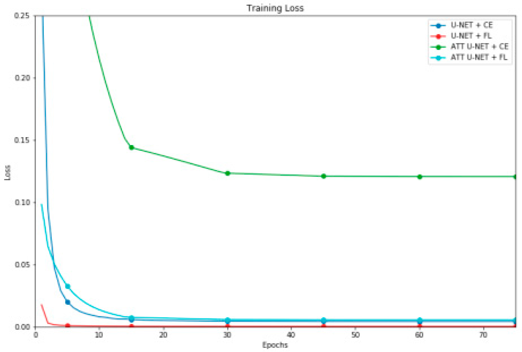
Analysis of the experimental outcomes from Table 3 for binary classification reveals in both of the architectures demonstrated enhanced segmentation outcomes with the CE loss function. Models trained with FL quickly converged and reached a premature local minimum within the initial ten epochs, thereby partially neglecting subsequent training. Figure 1 illustrates the loss function evolution graphs throughout the training process, highlighting the best segmentation performance for each model. The U-Net showcased superior segmentation outcomes for both loss functions. Comparing U-Net and Attention U-Net, both utilizing CE as the loss function, U-Net exhibited a slightly higher Accuracy (0.004%), Precision (0.574%), DSC (0.02%), and IoU (0.04%), whereas Attention U-Net displayed higher recall (0.536%). Notably, U-Net generated fewer FPs due to its higher precision, whereas Attention U-Net exhibited fewer FNs owing to its elevated recall, with other metrics showing comparable results. Attention U-Net models demonstrated lower standard deviation, with models employing the CE loss function also exhibiting reduced standard deviation. The Attention U-Net model with CE displayed the highest absolute percentage values of metrics during the training phase. Evaluating all metrics across the classification process for the four kidney segmentation models, the Attention U-Net model utilizing cross-entropy as the loss function emerged as the most proficient.

B. Multi Classification Results

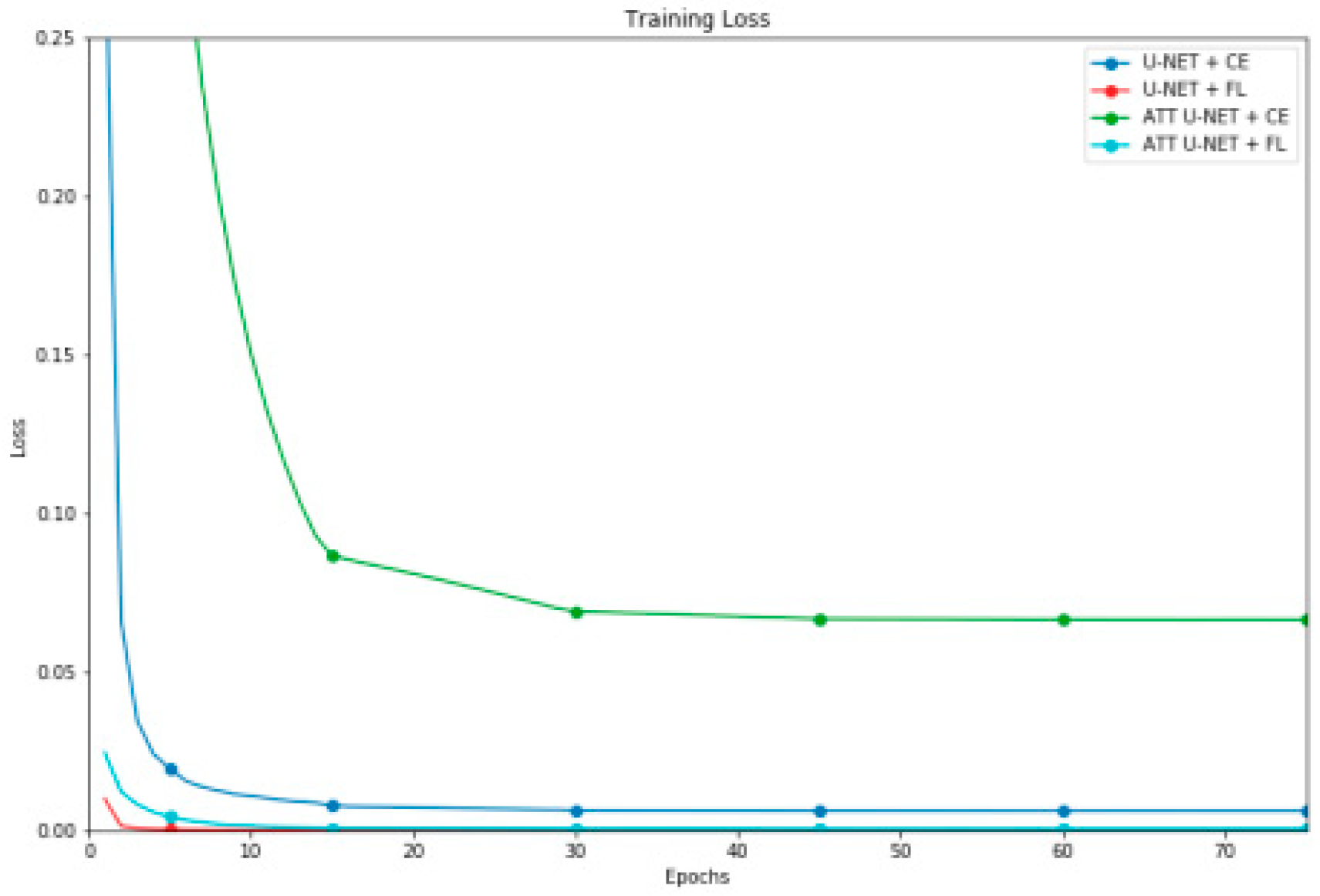
Upon examining the outcomes of the multi-class classification as presented in Table 4, several conclusions can be drawn that both architectures demonstrated improved segmentation outcomes when utilizing the CE loss function. Conversely, models trained with FL exhibited rapid convergence and reached a local minimum prematurely, predominantly overlooking subsequent stages of the training process. Graphs depicting the progression of the loss function throughout training, as illustrated in Figure 2, corroborate this observation, showcasing the superior segmentation performance achieved by each model. The Attention U-Net architecture yielded superior segmentation results across both loss functions. Attention U-Net models exhibited lower standard deviation values. Similarly, models employing the CE loss function displayed reduced standard deviation. The U-Net model utilizing the CE loss function showcased the highest absolute percentage metrics throughout the training phase. Upon evaluating the outcomes of all metrics employed in kidney segmentation across the four models, it is evident that the Attention U-Net model utilizing CE as its loss function yielded the most favorable segmentation results.

VI. Conclusion and Future Works

In summary, this study delved into the segmentation of kidneys in abdominal MRI scans utilizing the U-Net and Attention U-Net architectures. The objectives were met successfully, encompassing the development of a methodology for kidney segmentation, comparison between U-Net and Attention U-Net outcomes, examination of various loss functions, and investigation into binary and multi-class segmentation as a coarse-to-fine strategy. The findings indicate that the Attention U-Net model surpassed U-Net, showcasing advanced kidney segmentation capabilities. Among the evaluated functions, the CE loss function demonstrated superior performance, while the FL function warrants further exploration in parameterization. Binary segmentation exhibited enhanced results for smaller datasets and limited epochs, whereas multi-class segmentation incorporating a contour class did not notably enhance kidney segmentation. Notably, this study challenges conventional notions by revealing that extensive datasets and epochs are not indispensable for neural network training. These findings underscore the potential of the Attention U-Net architecture in the development of methodologies and tools leveraging kidney segmentation in abdominal MRI scans as a biomarker for kidney evaluation. Future research avenues may include optimizing the architecture's parameterization and investigating the efficacy of the FL function with refined parameters.

Funding

No funds, grants, or other support was received.

Data Availability

Data will be made on reasonable request.

Conflict of Interest

The authors declare that they have no known competing financial interests.

Code Availability

Code will be made on reasonable request.

References

  1. A. Rehman and F. G. Khan, “A deep learning based review on abdominal images,” Multimedia Tools and Applications 2020 80:20, vol. 80, no. 20, pp. 30321–30352, Sep. 2020. [CrossRef]
  2. D. Santhosh Reddy, P. Rajalakshmi, and M. A. Mateen, “A deep learning based approach for classification of abdominal organs using ultrasound images,” Biocybernetics and Biomedical Engineering, vol. 41, no. 2, pp. 779–791, Apr. 2021. [CrossRef]
  3. H. Arora and N. Mittal, “Image Enhancement Techniques for Gastric Diseases Detection using Ultrasound Images,” in Proceedings of the 3rd International Conference on Electronics and Communication and Aerospace Technology, ICECA 2019, Jun. 2019, pp. 251–256. [CrossRef]
  4. S. Maksoud, K. Zhao, P. Hobson, A. Jennings, and B. C. Lovell, “SOS: Selective objective switch for rapid immunofluorescence whole slide image classification,” in Proceedings of the IEEE Computer Society Conference on Computer Vision and Pattern Recognition, 2020, pp. 3861–3870. [CrossRef]
  5. C. M. Petrilli et al., “Factors associated with hospital admission and critical illness among 5279 people with coronavirus disease 2019 in New York City: Prospective cohort study,” The BMJ, vol. 369, May 2020. [CrossRef]
  6. K. D. Miller, M. Fidler-Benaoudia, T. H. Keegan, H. S. Hipp, A. Jemal, and R. L. Siegel, “Cancer statistics for adolescents and young adults, 2020,” CA: A Cancer Journal for Clinicians, vol. 70, no. 6, pp. 443–459, Nov. 2020. [CrossRef]
  7. V. Jurcak et al., “Automated segmentation of the quadratus lumborum muscle from magnetic resonance images using a hybrid atlas based - Geodesic active contour scheme,” in Proceedings of the 30th Annual International Conference of the IEEE Engineering in Medicine and Biology Society, EMBS’08 - “Personalized Healthcare through Technology,” 2008, pp. 867–870. [CrossRef]
  8. M. Byra et al., “Liver Fat Assessment in Multiview Sonography Using Transfer Learning With Convolutional Neural Networks,” Journal of Ultrasound in Medicine, vol. 41, no. 1, pp. 175–184, Jan. 2022. [CrossRef]
  9. A. Rehman and F. G. Khan, “A deep learning based review on abdominal images,” Multimedia Tools and Applications, vol. 80, no. 20, pp. 30321–30352, Aug. 2021. [CrossRef]
  10. Y. Kazemi and S. A. Mirroshandel, “A novel method for predicting kidney stone type using ensemble learning,” Artificial Intelligence in Medicine, vol. 84, pp. 117–126, Jan. 2018. [CrossRef]
  11. Q. Zheng, S. L. Furth, G. E. Tasian, and Y. Fan, “Computer-aided diagnosis of congenital abnormalities of the kidney and urinary tract in children based on ultrasound imaging data by integrating texture image features and deep transfer learning image features,” Journal of Pediatric Urology, vol. 15, no. 1, pp. 75.e1-75.e7, Feb. 2019. [CrossRef]
  12. P. Rathnayaka, V. Jayasundara, R. Nawaratne, D. De Silva, W. Ranasinghe, and D. Alahakoon, “Kidney Tumor Detection using Attention based U-Net,” 2019. [CrossRef]
  13. G. S. Kashyap, D. Mahajan, O. C. Phukan, A. Kumar, A. E. I. Brownlee, and J. Gao, “From Simulations to Reality: Enhancing Multi-Robot Exploration for Urban Search and Rescue,” Nov. 2023, Accessed: Dec. 03, 2023. [Online]. Available: https://arxiv.org/abs/2311.16958v1.
  14. S. Naz and G. S. Kashyap, “Enhancing the predictive capability of a mathematical model for pseudomonas aeruginosa through artificial neural networks,” International Journal of Information Technology 2024, pp. 1–10, Feb. 2024. [CrossRef]
  15. H. Habib, G. S. Kashyap, N. Tabassum, and T. Nafis, “Stock Price Prediction Using Artificial Intelligence Based on LSTM– Deep Learning Model,” in Artificial Intelligence & Blockchain in Cyber Physical Systems: Technologies & Applications, CRC Press, 2023, pp. 93–99. [CrossRef]
  16. G. S. Kashyap et al., “Detection of a facemask in real-time using deep learning methods: Prevention of Covid 19,” Jan. 2024, Accessed: Feb. 04, 2024. [Online]. Available: https://arxiv.org/abs/2401.15675v1.
  17. G. S. Kashyap, A. Siddiqui, R. Siddiqui, K. Malik, S. Wazir, and A. E. I. Brownlee, “Prediction of Suicidal Risk Using Machine Learning Models.” Dec. 25, 2021. Accessed: Feb. 04, 2024. [Online]. Available: https://papers.ssrn.com/abstract=4709789.
  18. G. S. Kashyap, K. Malik, S. Wazir, and R. Khan, “Using Machine Learning to Quantify the Multimedia Risk Due to Fuzzing,” Multimedia Tools and Applications, vol. 81, no. 25, pp. 36685–36698, Oct. 2022. [CrossRef]
  19. N. Marwah, V. K. Singh, G. S. Kashyap, and S. Wazir, “An analysis of the robustness of UAV agriculture field coverage using multi-agent reinforcement learning,” International Journal of Information Technology (Singapore), vol. 15, no. 4, pp. 2317–2327, May 2023. [CrossRef]
  20. G. S. Kashyap et al., “Revolutionizing Agriculture: A Comprehensive Review of Artificial Intelligence Techniques in Farming,” Feb. 2024. [CrossRef]
  21. S. Wazir, G. S. Kashyap, and P. Saxena, “MLOps: A Review,” Aug. 2023, Accessed: Sep. 16, 2023. [Online]. Available: https://arxiv.org/abs/2308.10908v1.
  22. M. Kanojia, P. Kamani, G. S. Kashyap, S. Naz, S. Wazir, and A. Chauhan, “Alternative Agriculture Land-Use Transformation Pathways by Partial-Equilibrium Agricultural Sector Model: A Mathematical Approach,” Aug. 2023, Accessed: Sep. 16, 2023. [Online]. Available: https://arxiv.org/abs/2308.11632v1.
  23. P. Kaur, G. S. Kashyap, A. Kumar, M. T. Nafis, S. Kumar, and V. Shokeen, “From Text to Transformation: A Comprehensive Review of Large Language Models’ Versatility,” Feb. 2024, Accessed: Mar. 21, 2024. [Online]. Available: https://arxiv.org/abs/2402.16142v1.
  24. G. S. Kashyap, A. E. I. Brownlee, O. C. Phukan, K. Malik, and S. Wazir, “Roulette-Wheel Selection-Based PSO Algorithm for Solving the Vehicle Routing Problem with Time Windows,” Jun. 2023, Accessed: Jul. 04, 2023. [Online]. Available: https://arxiv.org/abs/2306.02308v1.
  25. S. Wazir, G. S. Kashyap, K. Malik, and A. E. I. Brownlee, “Predicting the Infection Level of COVID-19 Virus Using Normal Distribution-Based Approximation Model and PSO,” Springer, Cham, 2023, pp. 75–91. [CrossRef]
  26. R. Arora, S. Gera, M. Saxena “Mitigating Security Riskon Privacy of Sensitive Data used in Cloud-based ERP Applications”; Proceedings of the 15th INDIACom; INDIACom-2021; IEEE Conference ID: 51348. 2021 8th International Conference on “Computing for Sustainable Global Development”, 17th - 19th March, 2021. pp 458-463 Electronic ISBN:978-93-80544-43-4. PoD ISBN:978-1-7281-9546-9.
  27. A. Soni, S.Alla, S.Dodda,H.Volikatla “Advancing Household.
  28. Robotics: Deep Interactive Reinforcement Learning for Efficient Training and Enhanced Performance,” in Journal of Electrical Systems (JES), vol. 20, no. 3s(2024), pp. 1349-1355 May 2024. [CrossRef]
1
Figure 1. Evolution of the loss function based on the resultant highest DSC for every binary class method.
Preprints 116142 g001
Figure 2. Evolution of the loss function based on the resultant highest DSC for every multi class method.
Preprints 116142 g002
Table 1. DATA AUGMENTATION TRANSFORMATIONS.
Transformation Parameters
Geometric Inversion Horizontal
Rotation [-5º, 5º]
Translation X axis: [-7%, 7%]
Y axis: [-3%, 3%]
Gray Scale Level Brightness [-10%, 40%]
Contrast [-10%, 40%]
Table 2. HYPERPARAMETERS USED.
Model
Parameters
U-Net Attention U-Net
Starting LR 10−2
LR decay drop = 0.1; Step decay = 15 epochs
Optimization Strategy Adam (β1 = 0.9, β2 = 0.999, ϵ = 10−7)
Epochs 75
Batch size 8
Dropout rate 0.1
Batch normalization True
Table 3. EVALUATION RESULTS OF THE BINARY CLASSES SEGMENTATION MODELS.
Segmentation Model DCS IoU Accuracy Precision Recall
U-NET + CE 0.966±0.009 0.934±0.016 0.997±0.001 0.967±0.012 0.965±0.019
U-NET + FL 0.960±0.011 0.923±0.020 0.997±0.001 0.980±0.010 0.941±0.023
ATT U-NET + CE 0.966±0.007 0.934±0.014 0.997±0.001 0.961±0.013 0.970±0.016
ATT U-NET + FL 0.944±0.094 0.902±0.094 0.996±0.004 0.970±0.096 0.920±0.095
Table 4. EVALUATION RESULTS OF THE MULTI CLASSES SEGMENTATION MODELS.
Segmentation Model DCS IoU Accuracy Precision Recall
U-NET + CE 0.937±0.015 0.888±0.024 0.995±0.002 0.936±0.019 0.956±0.020
U-NET + FL 0.936±0.016 0.887±0.024 0.995±0.002 0.935±0.020 0.938±0.014
ATT U-NET + CE 0.939±0.013 0.891±0.020 0.995±0.002 0.939±0.017 0.939±0.013
ATT U-NET + FL 0.937±0.015 0.889±0.024 0.995±0.002 0.937±0.019 0.939±0.015
Disclaimer/Publisher’s Note: The statements, opinions and data contained in all publications are solely those of the individual author(s) and contributor(s) and not of MDPI and/or the editor(s). MDPI and/or the editor(s) disclaim responsibility for any injury to people or property resulting from any ideas, methods, instructions or products referred to in the content.
Copyright: This open access article is published under a Creative Commons CC BY 4.0 license, which permit the free download, distribution, and reuse, provided that the author and preprint are cited in any reuse.
Prerpints.org logo

Preprints.org is a free preprint server supported by MDPI in Basel, Switzerland.

Subscribe

© 2024 MDPI (Basel, Switzerland) unless otherwise stated