Comparing the Efficiency of Particle Swarm and Harmony Search Algorithms in Optimizing the Muskingum-Cunge Model

Floods in various regions cause irreparable damage to infrastructure, agricultural lands, and industrial centers. In recent years, due to the effects of climate change and, in particular, the increased activity of the monsoon system in the Balochistan region located in southern Sistan and Baluchestan province, local rivers have overflowed, causing widespread flooding and significant damage. Accurate flood routing not only provides decision-makers with precise information about flood volume and flow behavior but also facilitates planning for effective preventive measures. In this study, the Muskingum-Cunge model was used to simulate floods in eight major rivers of Balochistan, including Kajou, Sarbaz, Nik Shahr, Kehir, Bahu, Sia Jangal, Rapch, and Kamb. The model parameters (K and X) were optimized using two machine learning algorithms: Particle Swarm Optimization (PSO) and Harmony Search (HS). The results showed that in most stations, the PSO algorithm outperformed HS. The algorithms were evaluated using the coefficient of residual mass (CRM), normalized root mean square error (NRMSE), efficiency (EF), and agreement index (d). For instance, at the Kajou station, PSO improved CRM by 0.017, Ef by 0.921, d by 0.982, and NRMSE by 0.099 compared to HS. At the Kamb station, both algorithms yielded comparable results. Considering the overall better performance of the PSO algorithm in most evaluation indices, it can be concluded that this algorithm is a more suitable option for optimizing the parameters of the Muskingum-Cunge model and simulating flood hydrographs with higher accuracy at most of the studied stations.

Keywords:

Subject: Engineering - Civil Engineering

1. Introduction:

Flood routing in channels and rivers is of paramount importance and is utilized in nearly all river engineering studies for flood control, involving unsteady flow computations[1-3]. Typically, during flood events, the main river channel fills, and floodwaters inundate floodplains. Under these conditions, the hydraulics of flow become highly complex due to the abrupt changes in flow velocity within the main channel and floodplains. The continuity and momentum equations, which form the basis of unsteady flow models, have limitations in such scenarios. Even using equations like the Saint-Venant equation, a cornerstone of flood routing, can lead to inaccuracies. These discrepancies may arise from model parameters that are sensitive to the basin’s geography and flow conditions[4-6]. Various mathematical methods have been proposed to refine these equations. Most of these methods introduce additional variables and parameters, increasing model complexity and computational time while improving accuracy. Simplified methods with minimal data requirements can be more practical. Unlike hydraulic models that employ numerical methods for flood routing and involve complex unsteady flow equations, hydrological models utilize a spatially lumped continuity equation and a storage equation for flood routing, requiring less data for flood prediction[7,8]. One such method is the Muskingum-Cunge model, renowned for its simplicity and accuracy, making it one of the most widely used hydrological routing models. However, determining optimal values for its parameters, especially the weighting coefficient, remains challenging.

1.1. Flood Routing Models and the Position of the Muskingum-Cunge Model

Flood routing is a critical aspect of hydrological studies and water resources management. Various models are employed to simulate and predict the behavior of flood flows in rivers and channels. These models can be broadly categorized into hydraulic and hydrological models. Hydraulic models are based on the numerical solution of unsteady flow differential equations, such as the Saint-Venant equations or continuity and momentum equations. Examples include the dynamic wave model, kinematic wave model, and diffusion wave model. While offering high computational accuracy, these models are complex, require extensive input data, and have long computation times [9,10]. In contrast, hydrological flood routing models utilize simpler and more approximate forms of flow equations. Notable examples include the Muskingum model, Clark model, and Muskingum-Cunge model. Hydrological models are characterized by their computational efficiency, limited data requirements, and simplicity. However, their accuracy is generally lower than that of hydraulic models [11,12]. Among hydrological flood routing models, the Muskingum-Cunge model holds a special place. This model, an extension of the original Muskingum model, combines the continuity equation with a simple storage equation to simulate flood flow over a time period. The Muskingum-Cunge model requires only two primary parameters, namely the time lag and weighting coefficient, which can be determined through calibration with observed data. Its simplicity and relatively good accuracy have made it one of the most widely used tools for hydrological routing.

1.2. Calibration Methods for Hydrological Models

Calibration of hydrological models, including the Muskingum-Cunge model, is a critical step in their application. Calibration involves determining optimal parameter values by comparing model outputs with observed data. For the Muskingum-Cunge model, the time lag and weighting coefficient must be adjusted to achieve the best fit between the simulated and observed hydrographs. Calibration methods can be broadly classified into manual and automated approaches. Manual calibration involves manually adjusting parameter values and comparing the output with real-world data. This is a time-consuming and tedious process, especially for models with numerous parameters. Automated methods, on the other hand, seek to find a set of parameters that minimizes an objective function, such as the sum of squared errors, thereby achieving the best fit with observed data.Various automated calibration methods exist, each with its own advantages and disadvantages. One popular approach involves the use of evolutionary optimization algorithms, which have gained significant attention in recent years [12].

1.3. Application of Optimization Algorithms in Solving Hydrological Problems

Evolutionary optimization algorithms, such as genetic algorithms, particle swarm optimization, harmony search, and ant colony optimization, have demonstrated remarkable capabilities in solving complex multi-variable optimization problems. Consequently, their application in hydrological problems, including model calibration, parameter estimation, and water resources systems optimization, has garnered significant attention from researchers. Flood routing is a critical issue in the design and evaluation of hydraulic structures, water resources planning, and forecasting river flow and maximum water levels. Since most rivers lack continuous monitoring stations, methods are needed to estimate flow and water levels at specific locations. Flood routing is therefore used to assess flood wave profiles along a river and gain a better understanding of flood flow characteristics. Moreover, flood management can be viewed as risk management, involving measures to reduce the risk of floods or mitigate their impacts, such as minimizing damage to infrastructure, residential areas, and loss of life [13]. Generally, flood routing methods can be categorized into hydraulic and hydrological methods[14]. Hydraulic methods are based on the solution of differential continuity and momentum equations. While offering high accuracy, hydraulic methods require data such as flow depth, velocity, roughness coefficient, cross-sectional area, and bed slope [15]. Collecting such data is time-consuming and costly. However, hydraulic methods are relatively simple and reasonably accurate, requiring only one or more simultaneous input or output hydrographs from a gauging station [13]. The Muskingum method is one of the most well-known and widely used hydrological flood routing techniques. In this method, model parameters (decision variables) are estimated through optimization methods based on historical input-output hydrograph data. Then, the Muskingum routing equations are executed to determine an output hydrograph corresponding to an input hydrograph [16]. The Muskingum method can be applied to river routing in both linear and nonlinear forms. In the linear model, a linear relationship between storage and discharge is assumed, and subsequent calculations are based on this assumption. The linear Muskingum model has been used by various researchers [17,18]. Since the storage-discharge relationship is generally nonlinear[19], the linear Muskingum model may not provide sufficient accuracy in simulating floods. Therefore, Gill (1978) introduced a nonlinear version of the Muskingum method. The existence of a nonlinear relationship between storage and discharge in a river system is closer to reality and seems more logical. Consequently, the nonlinear Muskingum method has gained more attention from researchers in recent years [14,20,21]. Comparisons between the Muskingum-Cunge and kinematic wave methods have shown that, although the kinematic wave method utilizes more accurate data, the Muskingum-Cunge method is more efficient for flood routing. This efficiency is attributed to its lower data requirements and the generation of hydrographs that closely resemble real-world data compared to the kinematic wave method[22]. A four-parameter nonlinear Muskingum model has also been proposed, demonstrating more accurate predictions of flood discharge compared to the three-parameter model [23]. Moradi et al. (2008) applied both the Muskingum and Muskingum-Cunge methods to a section of the Liqvan River and compared the results for floods with return periods of 2, 10, 20, 50, and 100 years. The results revealed differences between the routing results of the two models and actual values. Fotuhi and Maghrebi (2010) compared dynamic and Muskingum-Cunge routing in a channel study and found minimal differences between the two methods. However, they cautioned against using the Muskingum-Cunge method in low-gradient channels. Norouzi and Bazargan (2020) investigated the accuracy of the Muskingum-Cunge method between the Malthan and Ahvaz gauging stations along the Karun River. Their findings indicated that the parameters of the Muskingum-Cunge method performed better when using three different values instead of a single constant value. This study aims to develop a model for the Balochistan region, prone to seasonal river flooding during monsoon seasons, using well-established algorithms and an optimization process. Given the limited data availability from flow gauging stations in Balochistan’s rivers, the Muskingum-Cunge model, which requires minimal data, is employed. Furthermore, to address the challenge of parameter estimation in the routing process, metaheuristic algorithms such as Particle Swarm Optimization (PSO) and Harmony Search Algorithm (HSA) will be utilized in conjunction with a three-parameter Muskingum model to optimize the routing in eight flood-prone rivers within the region.

2. Materials and Methods

2.1. Study Area

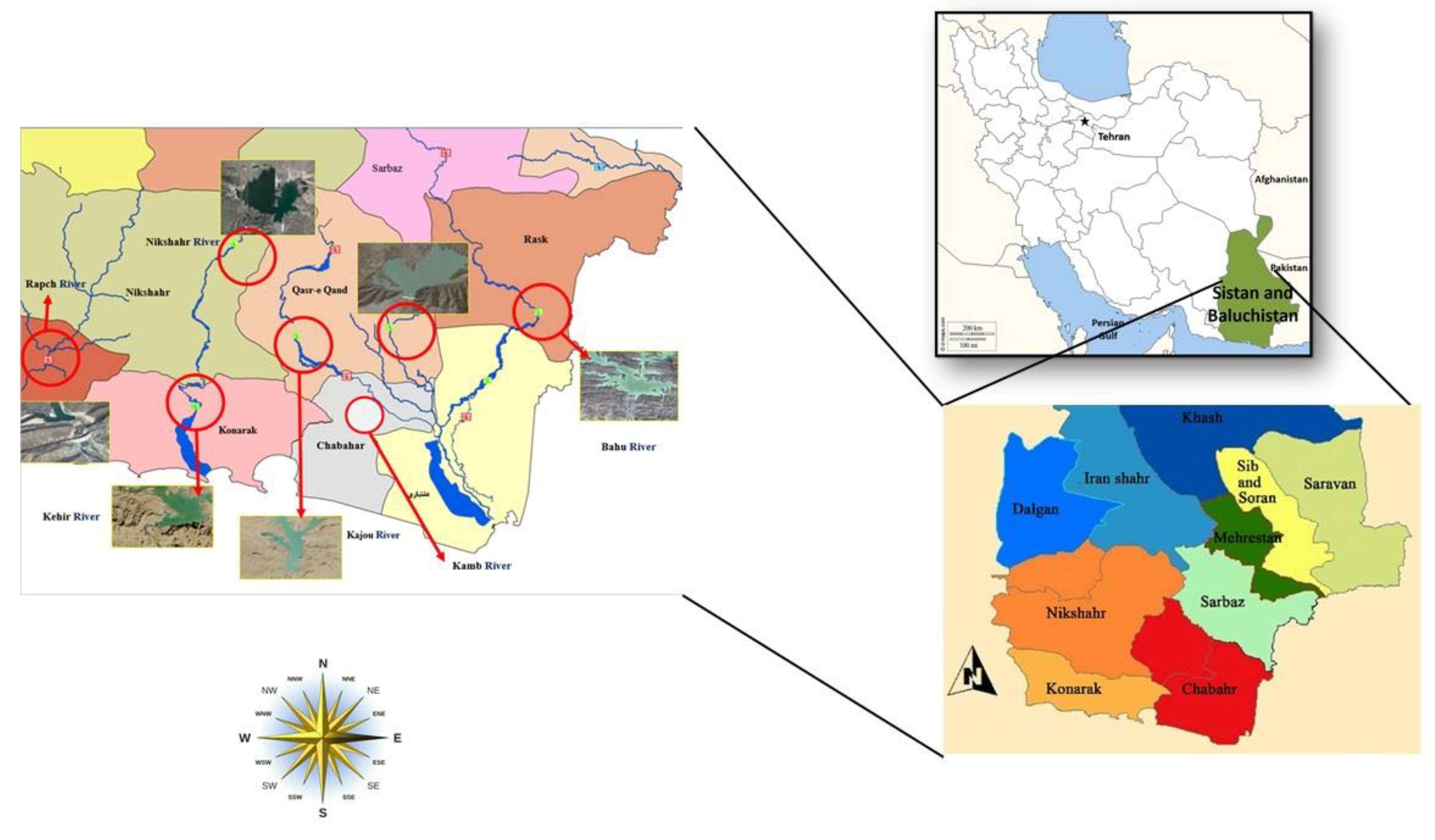
Sistan and Baluchestan province, spanning 180,726 square kilometers, is located in southeastern Iran, between 25°3’ and 31°27’ north latitude and 58°50’ and 63°21’ east longitude. The province comprises two main regions: northern Sistan and southern Baluchestan. It is divided into 15 counties (Zahedan, Mirjaveh, Khash, Saravan, Iranshahr, Nik Shahr, Chabahar, Sarbaz, Konarak, Delgan, Mehrestan, Sib and Soran, Bampoor, Qasr-e Qand, and Fanuj) (Statistical Center of Iran, 2020). This research focuses on the Baluchestan region, utilizing data collected from hydrometric stations along the Rapch, Sarbaz, Kehir, Siahjangal, Bahu, Kajou, Nikshahr, and Kamb rivers to conduct flood routing using the Muskingum-Cunge method (Figure 1). The characteristics of the studied rivers and their basins are presented in Table 1. These data will be used to construct inflow hydrographs for the river basins in the study area. Given the region’s vast geographical extent, it exhibits a diverse climate. Climate zoning indicates that the counties of Nikshahr, Qasr-e Qand, Mirjaveh, Konarak, Chabahar, Sarbaz, and Iranshahr have arid hot desert, semi-arid temperate, arid hot coastal, and extremely arid hot desert climates, respectively (Moradi et al., 2020). The region is characterized by high average temperatures (22.6°C) and low temperature fluctuations. Due to low annual precipitation (139.8 mm) and the absence of mountainous snow sources, most river flows are seasonal and temporary. In many parts of Baluchestan, limited groundwater resources serve as the primary water supply [12].

2.2. The Muskingum-Cunge Method

The Muskingum method, initially proposed in 1938 based on studies of the Muskingum River in the United States, is a linear model founded on the continuity equation (McCarthy, 1939). The model is represented by the following equations:

\frac{d s_{t}}{d t} = I_{t} - O_{t}

(1)

S_{t} = K [x I_{t} + (1 + x) O_{t}]

(2)

where:

S_t is the storage volume of the river (m³), I_t is the inflow rate (m³/s), Q_t is the outflow rate (m³/s)

K is the storage time constant (s), varying between 0 and 30 x is the weighting factor, ranging from 0 to 0.5

In 1969, Cunge demonstrated that this equation is analogous to the advection-dispersion equation and that its results closely resemble those obtained from the kinematic wave method. By modifying the kinematic wave equation and aligning physical diffusion with numerical diffusion, Cunge refined the Muskingum equation. The resulting modified Muskingum-Cunge equation, capable of considering lateral inflows, can be calculated based on the river’s physical characteristics (Cunge, 1969). This method has been widely used for flood routing in various regions. Assuming that inertia and acceleration can be neglected compared to the bottom slope in natural channels, Cunge proved that the advection-dispersion equation is similar to the Muskingum equation. Based on this, the Muskingum-Cunge equation for flood routing can be defined as follows (Cunge, 1969):

Q_{i + 1}^{j + 1} = α_{1} Q_{i}^{j + 1} + α_{2} Q_{i}^{j} + α_{3} Q_{i + 1}^{j}

(3)

where the coefficients

α_{1}, α_{2},

and

α_{3}

can be calculated using equations (4) to (6) (Chow, 1959):

α_{1} = \frac{Δ t - 2 K X}{2 K (1 - X) + Δ t}

(4)

α_{2} = \frac{Δ t + 2 K X}{2 K (1 - X) + Δ t}

(5)

α_{3} = \frac{2 K (1 - X) - Δ t}{2 K (1 - X) + Δ t}

(6)

In these equations, Δt is the time step, Δx is the spatial step, and K and x are routing parameters. It should be noted that the sum of

α_{1}, α_{2},

and

α_{3}

is equal to 1, and both K and Δx have units of time. In the above equations, K is the storage constant, and x is a factor that represents the relative influence of inflow on storage and is dimensionless. Cunge showed that when K and x are assumed to be constant, equation (3) is an approximate solution to the kinematic wave equations. Additionally, this equation is also an approximate solution to the diffusion equation in a channel. Therefore, the values of the routing parameters K and x can be calculated using the following equations:

K = \frac{Δ X}{C_{K}} = \frac{Δ X}{\frac{d Q}{d A}}

(7)

X = \frac{1}{2} (1 - \frac{Q}{B C_{K} S Δ x})

(8)

where

C_{K}

is the wave celerity related to the flood discharge, B is the water surface width in the river or channel, Q is the reference discharge, and Δx is the spatial step. The reference discharge is the discharge used to accurately estimate the routing parameters (Akbari et al., 2010). Equation (8) shows that the value of x is directly related to the reference discharge, which is a function of the inflow. Since the inflow varies during a flood event, the reference discharge also varies. Therefore, in the constant parameter Muskingum-Cunge method, the reference discharge is considered constant in all computational cells. In this study, the following equation is used to estimate the reference discharge (Akan et al., 2006; Wilson & Ruffini, 1988):

Q = Q_{b} + 0.5 (Q_{P i} - Q_{b})

(9)

where Q_b and Q_pi represent the minimum and maximum inflow rates, respectively.

It is observed that estimating the routing parameters K and x is the most critical part of flood routing estimation, and traditional manual methods are time-consuming. Therefore, modern methods based on artificial intelligence should be used to estimate these parameters, as they are more accurate and time-efficient. In this study, two optimization algorithms, particle swarm optimization (PSO) and harmony search (HS), will be used to estimate these parameters and find the best solution. The programming of these machine learning algorithms will be done in the MATLAB programming environment.

2.2. Particle Swarm Optimization (PSO)

PSO is an evolutionary algorithm introduced in 1995. Based on population-based search, similar to genetic algorithms, ant colony optimization, and bee colony optimization, PSO is a nature-inspired algorithm that mimics the collective intelligence and social behavior of birds and fish [24,25]. Due to its simple structure, few controllable parameters, rapid convergence, and high computational efficiency, PSO is widely used in optimization problems. Although primarily developed for optimization problems with continuous variables, PSO has been successfully adapted for discrete variable problems. In PSO, each solution is considered a bird in a flock and is termed a particle. These particles exhibit both individual intelligence and social behavior, coordinating their movement towards a target (Montalvo et al., 2008). The process begins with a swarm of particles, each representing a randomly generated solution to the problem. The swarm then iteratively searches for the optimal solution. Each particle i is defined by three vectors: its current position Xi, its best previous position Yi, and its velocity Vi.

X_{i} = (x_{i 1}, x_{i 2} ..... x_{i n}) current position

(10)

| Y_{i} = (y_{i 1}, y_{i 2} ..... y_{i n}) Best previous position

(11)

V_{i} = (v_{i 1}, v_{i 2} ..... v_{i n}) Flight velocity

(12)

It is assumed that the simulated bird flock communicates while flying, and each bird looks towards a specific direction, which is the best position achieved (Yi) in the current state. Subsequently, when the birds communicate, the bird in the best position is identified. Through coordination, each bird moves towards the best bird with a velocity that depends on its current velocity. Therefore, each bird explores the search space from its current local position, and this process repeats until the bird potentially reaches the desired position. Birds learn through their own experience (local search) and the experience of their peers (global search). In each iteration, the particle with the best momentary solution to the problem is identified. The position of this particle is then used in calculating the new position for each particle in the swarm. This calculation is based on the following equation:

X_{i, d}^{n + 1} = X_{i, d}^{n} + V_{i, d}^{n + 1}

(13)

The best position achieved by each particle in each swarm is denoted by p-best, and the best position achieved in the entire population is denoted by g-best. Ultimately, the coordinated population moving in one direction is represented by the following equation:

V_{i, d}^{n + 1} = ω V_{i, d}^{n} + c_{1} r_{1}^{n} (p b e s t_{i, d}^{n} - X_{i, d}^{n}) + c_{2} r_{2}^{n} (g b e s t_{i, d}^{n} - X_{i, d}^{n})

(14)

where d=1, 2, …, D, i=1, 2, …, N, N is the population size, ω is the inertia weight, c₁ and c₂ are positive constant coefficients that refer to cognitive and social parameters (learning factors), respectively, r1 and r2 are random numbers between 0 and 1, and n=1, 2, … denotes the number of iterations [26].

Furthermore, inertia weight is an index to ensure the convergence behavior of PSO, which is used to control the effect of the history of velocities on the current velocity. This coefficient may change from one iteration to the next. Since this coefficient controls the balance between global and local search, it is suggested to decrease linearly with time, usually in a way that global search is prioritized at the beginning and local search is prioritized with each subsequent iteration[27]. To determine the inertia weight, the following equation is used:

w = w_{\max} - \frac{(w_{\max} - w_{\min}) \times n}{i T e r_{\max}}

(15)

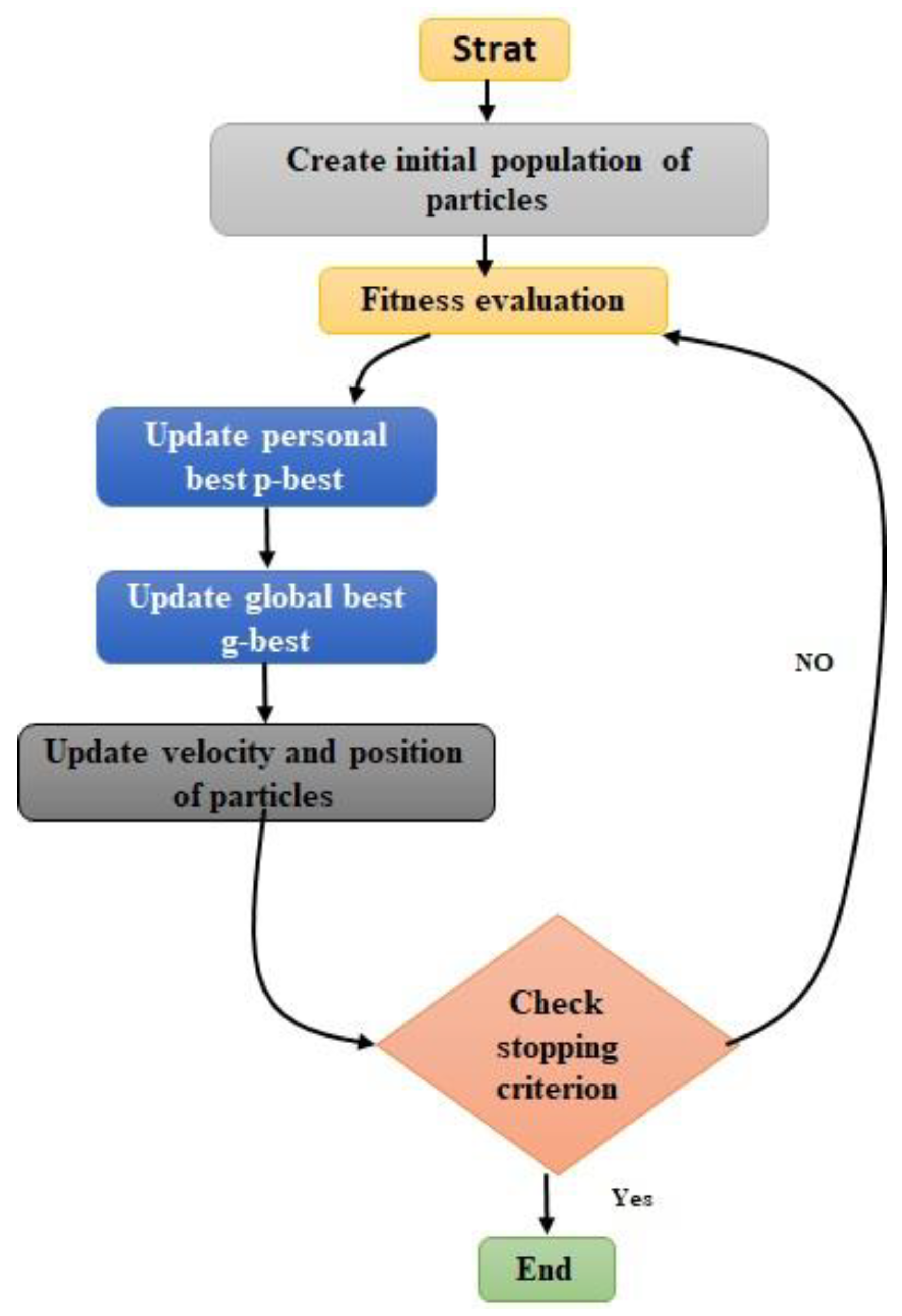
where ωmax is the initial inertia, ωmin is the final inertia, iTer_max is the maximum number of iterations, and n is the current iteration number. According to experimental studies, the best values for ωmax and ωmin are 0.9 and 0.4, respectively [28]. Although the constant coefficients c1 and c2 do not have a decisive role in the convergence of PSO, by determining appropriate initial values, it is possible to increase the convergence speed and improve the local solution. The suggested initial values for these coefficients also show that choosing a larger cognitive parameter (c1) compared to the social parameter (c2), with the condition c1 + c2 ≤ 4, leads to better results. The flowchart of the particle swarm optimization algorithm is shown in Figure 2

3.2. Harmony Search Algorithm: A Musical Inspiration

The Harmony Search (HS) metaheuristic algorithm draws inspiration from the musical process of searching for a state of “perfect” harmony, akin to jazz improvisation [29]. Jazz improvisation seeks the optimal state (a superb harmony) as determined by aesthetic evaluation, just as an optimization algorithm seeks the optimal state (global optimum) as determined by an objective function evaluation. Aesthetic evaluation is performed by the set of notes played by each instrument, similar to how the objective function is evaluated by a set of values determined by each decision variable. The quality of the harmony improves with consistent practice, just as the quality of the solution improves with iterations.

Key Advantages of HS:

Ability to handle discrete variables: Unlike many numerical optimization methods, HS can effectively handle discrete variables, reducing the likelihood of getting trapped in local optima [30,31].

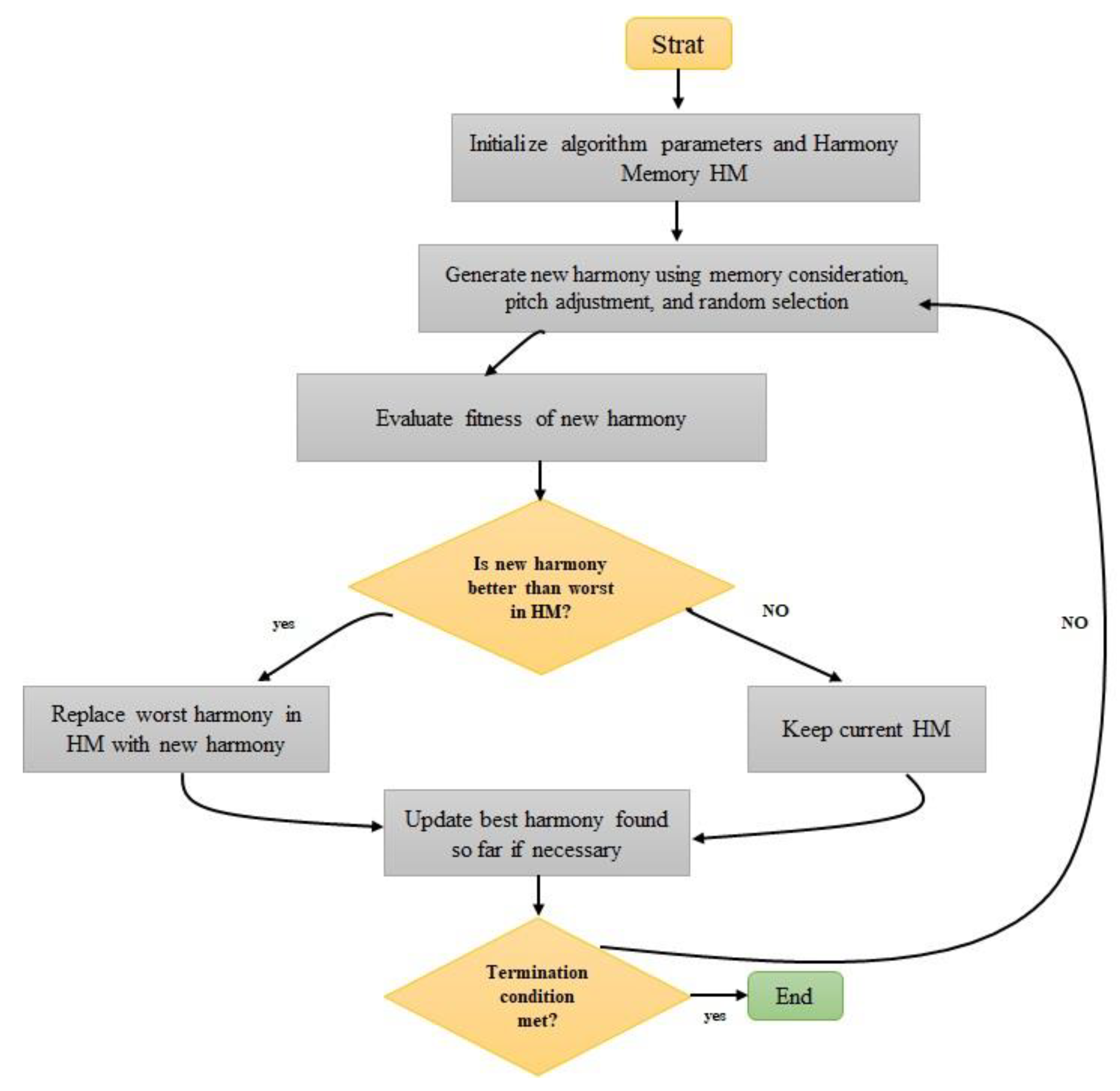
Steps Involved in the HS Algorithm:

Initialization: Set initial values for algorithm parameters such as Harmony Memory Size (HMS), Harmony Memory Considering Rate (HMCR), Pitch Adjusting Rate (PAR), and generate an initial harmony.

Initialization of Harmony Memory (HMS): Populate the HMS with a set of randomly generated harmony vectors.

Creating a new harmony using HMS: For each variable of a new harmony vector, three operators are employed: HMCR, PAR, and random selection.

-: HMCR: If a random number is less than HMCR, a value is selected from the HMS.
-: PAR: If a random number is less than PAR, the selected value is slightly adjusted.
-: Random selection: If neither HMCR nor PAR conditions are met, a random value within the variable’s bounds is selected.

Updating the Harmony Memory: Evaluate the new harmony using the objective function. If it’s better than the worst harmony in the HMS, replace the worst harmony with the new one.

Termination: Check if the termination criterion (e.g., maximum number of iterations) is met. If not, go back to step 3.

Here’s the translation and formulas for the evaluation metrics of machine learning algorithms:

3. Evaluation of Machine Learning Algorithm Performance

To evaluate the algorithms used, the following indices were employed: Coefficient of Residual Mass (CRM), Normalized Root Mean Square Error (NRMSE), Model Efficiency (EF), and Index of Agreement (d) [32,33].

1. Coefficient of Residual Mass (CRM):

CRM = (Σ Oi - Σ Pi) / Σ Oi

(16)

2. Normalized Root Mean Square Error (NRMSE):

NRMSE = √[(Σ (Pi - Oi)²) / n] / Ō

(17)

3. Model Efficiency (EF):

EF = 1 - [Σ (Oi - Pi)² / Σ (Oi - Ō)²]

(18)

4. Index of Agreement (d):

d = 1 - [Σ (Pi - Oi)² / Σ (|Pi - Ō| + |Oi - Ō|)²]

(19)

where:

Oi: Observed values, Pi: Predicted values, Ō: Mean of observed values, n: Number of observations

These metrics provide a comprehensive evaluation of the model’s performance, including its bias (CRM), accuracy (NRMSE), efficiency (EF), and overall agreement with observed data (d). NRMSE (Normalized Root Mean Square Error) represents the difference between simulated and observed data relative to the mean of observed data. For this index:

-: Values less than 10%: Excellent
-: Values between 10% and 20%: Good
-: Values between 20% and 30%: Fair
-: Values greater than 30%: Poor

The EF (Model Efficiency) index indicates the degree of alignment between observed and predicted plots with the 1:1 line. Its values range from 1 to negative infinity. An EF value of 1 corresponds to a perfect fit [34]. The d (Index of Agreement) ranges from 0 to 1:

-: 1 indicates perfect agreement between simulated and observed data
-: 0 indicates no agreement
-: For CRM (Coefficient of Residual Mass):
-: Positive values indicate underestimation of crop performance
-: Negative values indicate overestimation of crop performance

These metrics collectively provide a comprehensive evaluation of model performance, assessing accuracy, bias, and agreement between predicted and observed values. Finally, in addition to examining and evaluating the performance of the Muskingum-Cunge model for estimating the flood input hydrograph in the Baluchistan region, the routing parameters in this model are estimated using machine learning algorithms. By comparing these machine learning methods, the best approach for this region is determined for estimating the flood input hydrograph and its routing.

4. Results and Discussion

This study aims to find the optimal parameters (K and X) for the Muskingum-Cunge model using PSO and HS algorithms. The performance of these two algorithms in terms of convergence rate, accuracy, and objective function values is compared. The results of both algorithms, including convergence trends and optimal parameter values, are presented and discussed.

This Table 2. presents initial estimates for parameters X and K for eight rivers, derived using Particle Swarm Optimization (PSO) and Harmony Search (HS) algorithms. The results show similar values between PSO and HS for most rivers, suggesting consistency across methods. Parameter X values are relatively stable across all rivers, ranging from about 0.16 to 0.43. In contrast, parameter K shows greater variation, with values from 2.85 to 29.11.

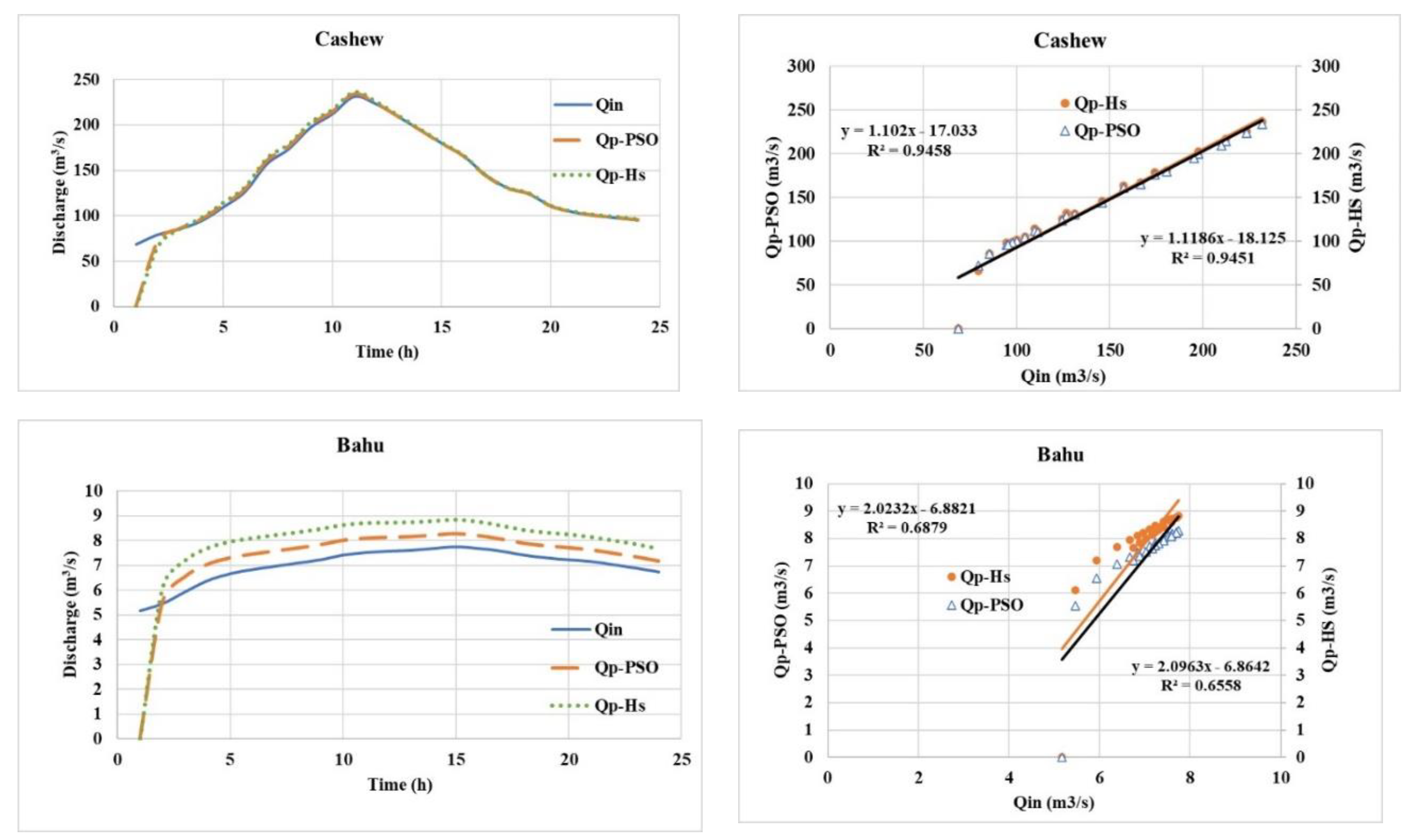
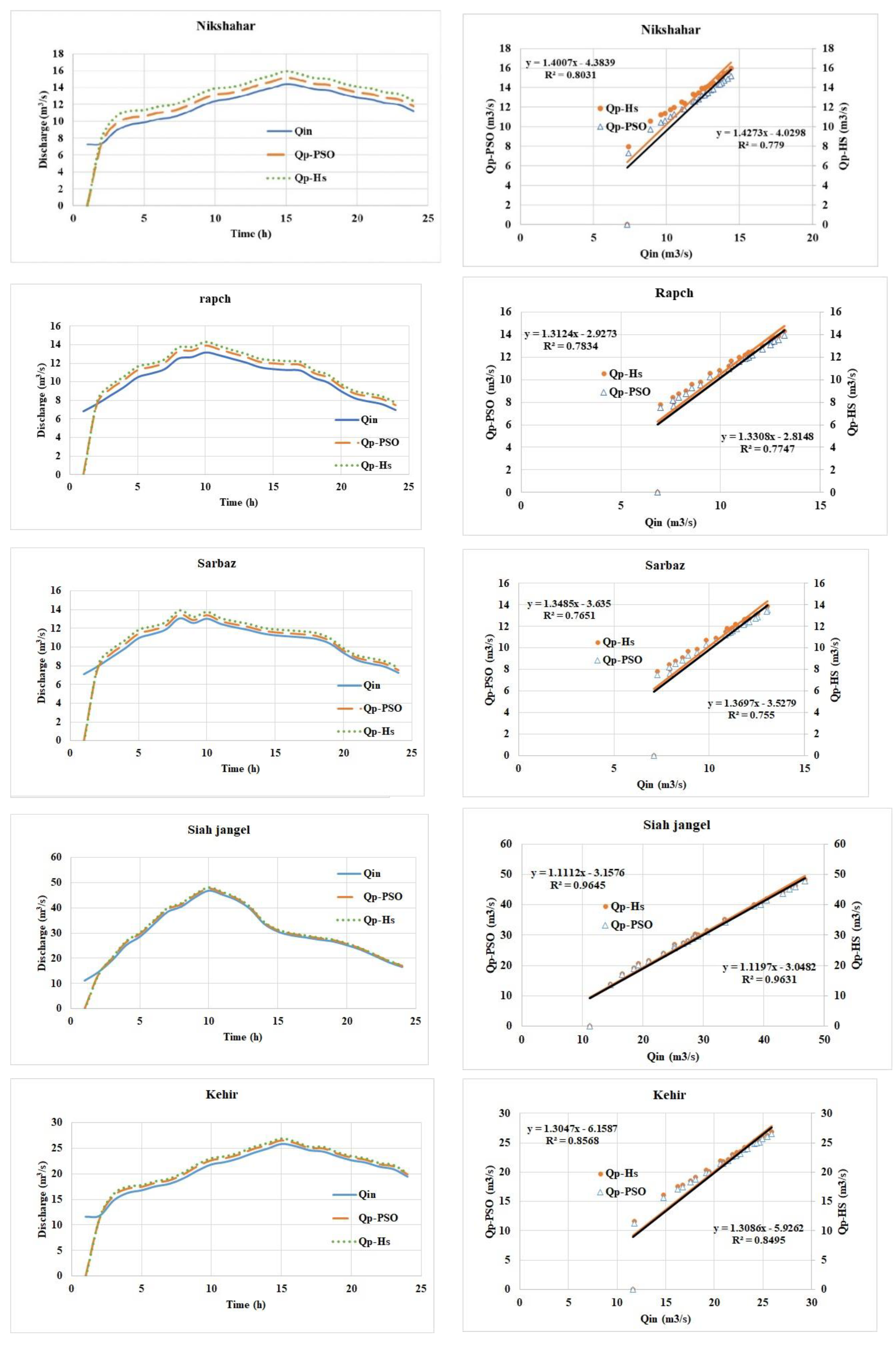
Figure 4, presents a Comparison of PSO and HS Optimization Models with Actual Flood Discharge Data This analysis compares the results from Particle Swarm Optimization (PSO) and Harmony Search (HS) optimization models with actual flood discharge data across multiple stations. The performance of these models was evaluated using correlation coefficients (R²) and visual comparison of simulated hydrographs with actual flood discharge data.

Kajoo Station: Both PSO and HS models simulated the flood discharge with high accuracy. Peak discharge values were 231.60, 234.07, and 236.52 m³/s for actual, PSO, and HS models respectively. Correlation coefficients were exceptionally high at 0.9458 (PSO) and 0.9451 (HS), indicating very strong correlation between simulated and actual data.

Bahu Station: Both algorithms successfully simulated the flood output hydrograph with acceptable accuracy. The simulated graphs closely matched the actual flood discharge graph. Correlation coefficients were 0.6879 for PSO and 0.6558 for HS, which are close to 0.7, indicating acceptable correlation between simulated and actual data.

Nikshahr Station: The algorithms simulated the flood hydrograph with acceptable accuracy. Correlation coefficients were 0.8031 for PSO and 0.7790 for HS, showing moderate to good correlation.

Rapch Station: Simulated hydrographs closely matched actual flood discharge. Correlation coefficients of 0.7834 (PSO) and 0.7747 (HS) demonstrated moderate to good correlation.

Sarbaz Station: Both algorithms provided acceptable accuracy, with correlation coefficients of 0.7651 (PSO) and 0.755 (HS), showing moderate to good correlation.

Siah Jangal Station: This station showed the highest correlation among all stations, with coefficients of 0.9645 (PSO) and 0.9631 (HS), indicating very high agreement between simulated and actual data.

Kahir Station: Both algorithms achieved highly accurate simulation, with correlation coefficients of 0.8568 (PSO) and 0.8495 (HS), showing very good correlation.

Kamb Station: While overall simulation was acceptable, both algorithms struggled to accurately simulate flood discharge during certain time periods, resulting in significant differences between simulated and actual data in these instances.

In conclusion, both PSO and HS optimization algorithms demonstrated good overall performance in simulating flood hydrographs across the studied stations. The Siah Jangal station showed the highest correlation, while the Bahu and Kamb stations presented some challenges in accurately simulating certain aspects of the flood discharge. These results suggest that both PSO and HS are effective tools for flood discharge simulation, although their performance may vary depending on the specific characteristics of each station and time period.

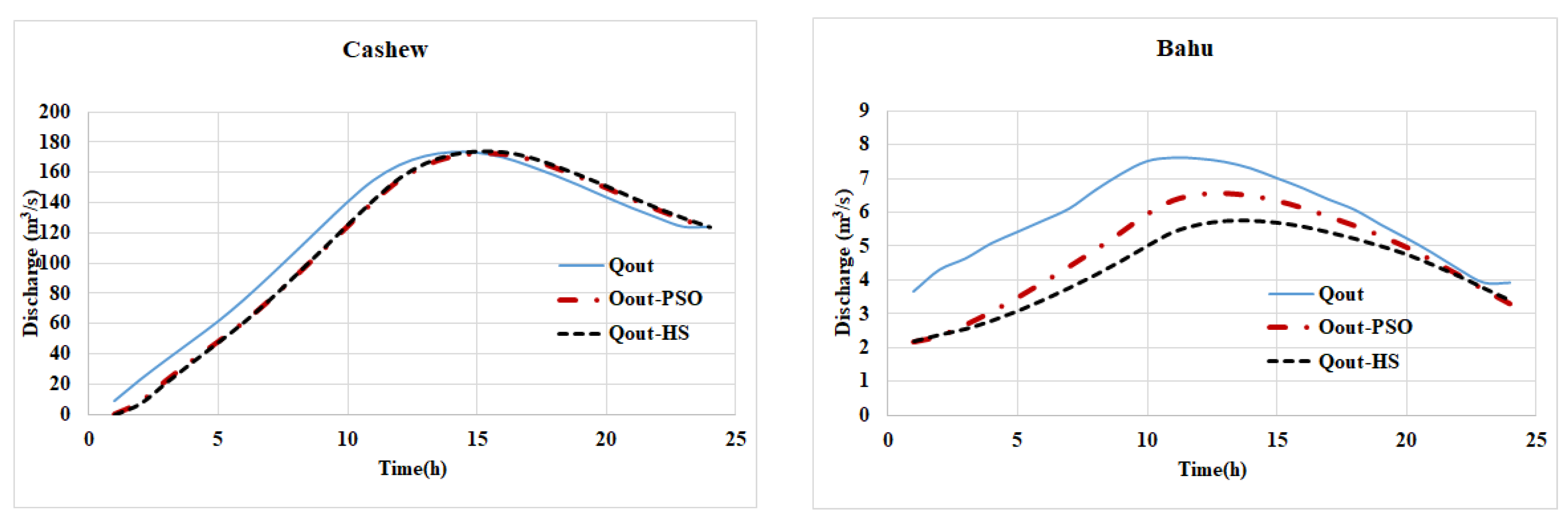
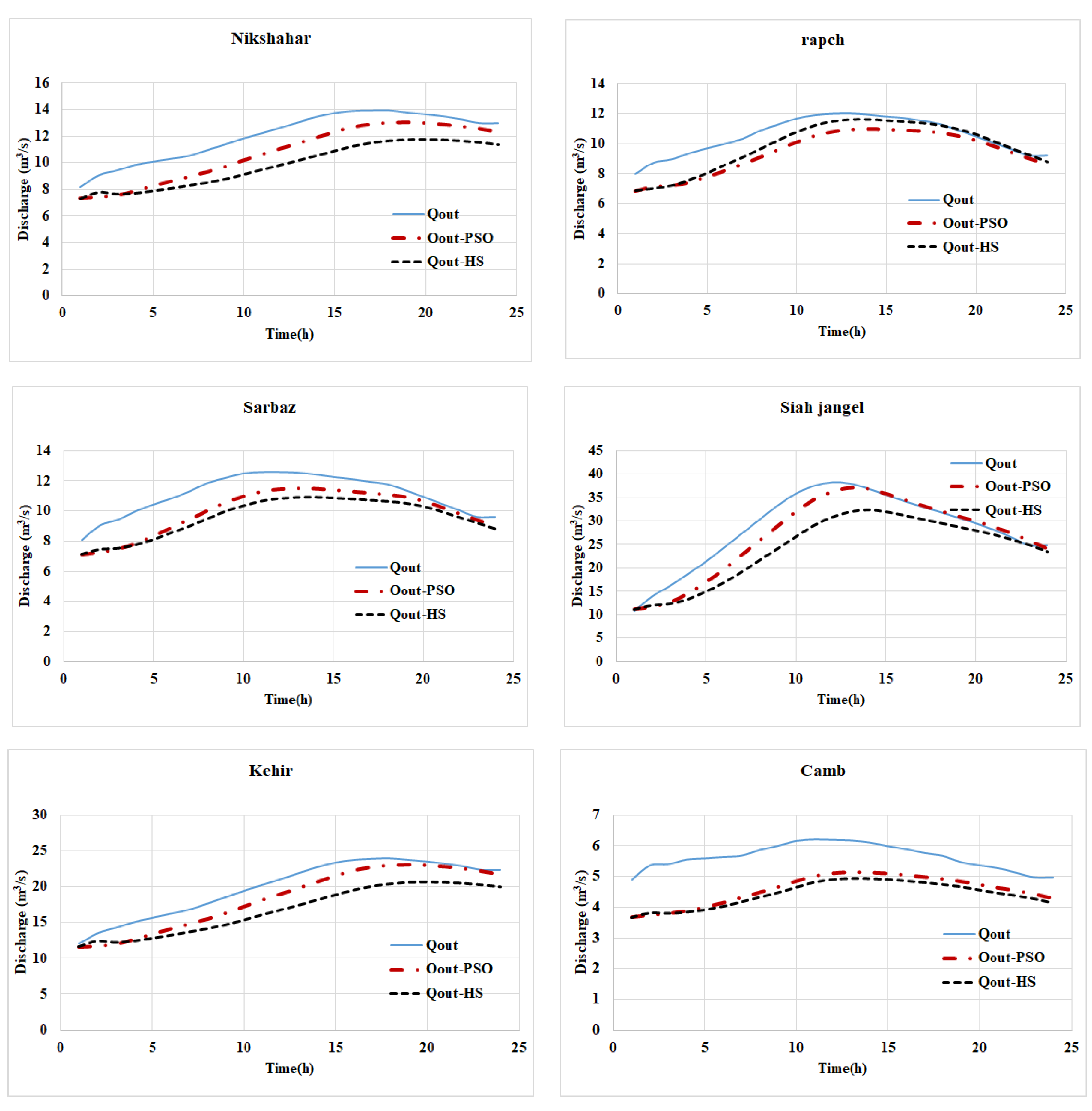
Figure 5 illustrates the charts of inlet flow and outlet flow with PSO and HS models, optimizing the Muskingum-Cunge coefficients for various stations. Kajo Station: The chart shows the input and output discharge using coefficients optimized by PSO and HS models. Peak outflow discharge values for PSO and HS models were 172.45 and 174.10 cubic meters per second, respectively, indicating acceptable accuracy for both models in simulating the outflow discharge. Bahu Station: Both PSO and HS algorithms, by optimizing Muskingum-Cunge coefficients, have simulated the flood outflow discharge with acceptable accuracy. The simulated outflow discharge graphs for both algorithms are close to each other. NikShahr Station: The optimization of Muskingum-Cunge coefficients by both PSO and HS algorithms has resulted in acceptable accuracy in simulating flood outflow discharge. The simulated outflow discharge graphs for both algorithms are similar. Rapch Station: Both PSO and HS algorithms have successfully optimized Muskingum-Cunge coefficients, leading to acceptable accuracy in simulating flood outflow discharge. The simulated outflow discharge graphs for both algorithms are close to each other. Sarbaz Station: The optimization of Muskingum-Cunge coefficients by PSO and HS algorithms has produced acceptable accuracy in simulating flood outflow discharge. The simulated outflow discharge graphs for both algorithms show close agreement. Siyah Jangal Station: Both PSO and HS algorithms have optimized Muskingum-Cunge coefficients very effectively, resulting in highly accurate simulation of flood outflow discharge. The simulated outflow discharge graphs for the two algorithms show very close alignment with each other. Kahir Station: The optimization of Muskingum-Cunge coefficients by PSO and HS algorithms has led to good accuracy in simulating flood outflow discharge. The simulated outflow discharge graphs for the two algorithms show good agreement, indicating similar performance. Kamb Station: Both PSO and HS algorithms have successfully optimized Muskingum-Cunge coefficients, resulting in good accuracy in simulating flood outflow discharge. The simulated outflow discharge graphs for the two algorithms show good agreement, demonstrating good and similar performance. Overall, these results confirm that both PSO and HS algorithms perform well in optimizing Muskingum-Cunge coefficients across various stations, producing accurate simulations of flood outflow discharge.

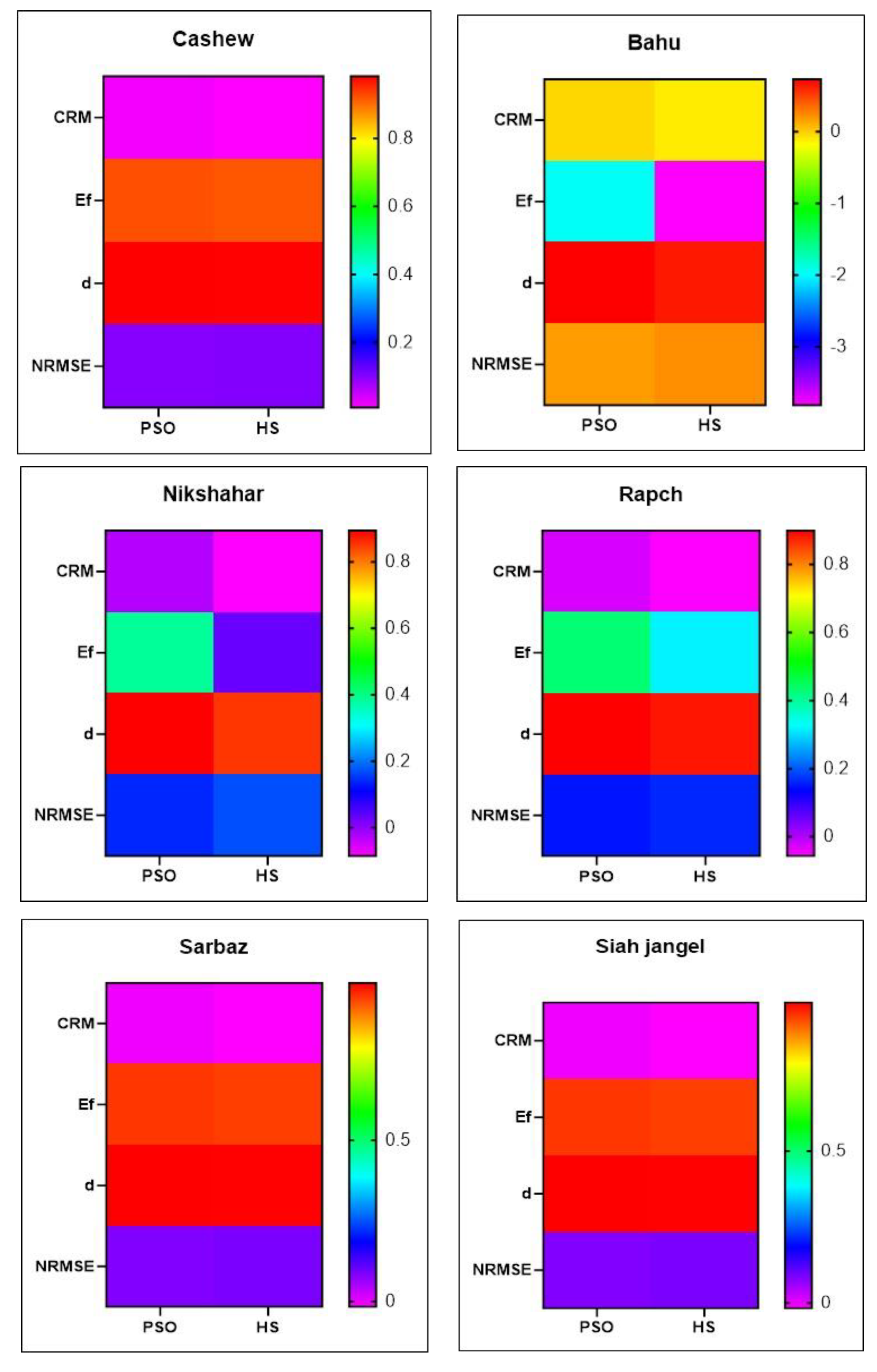
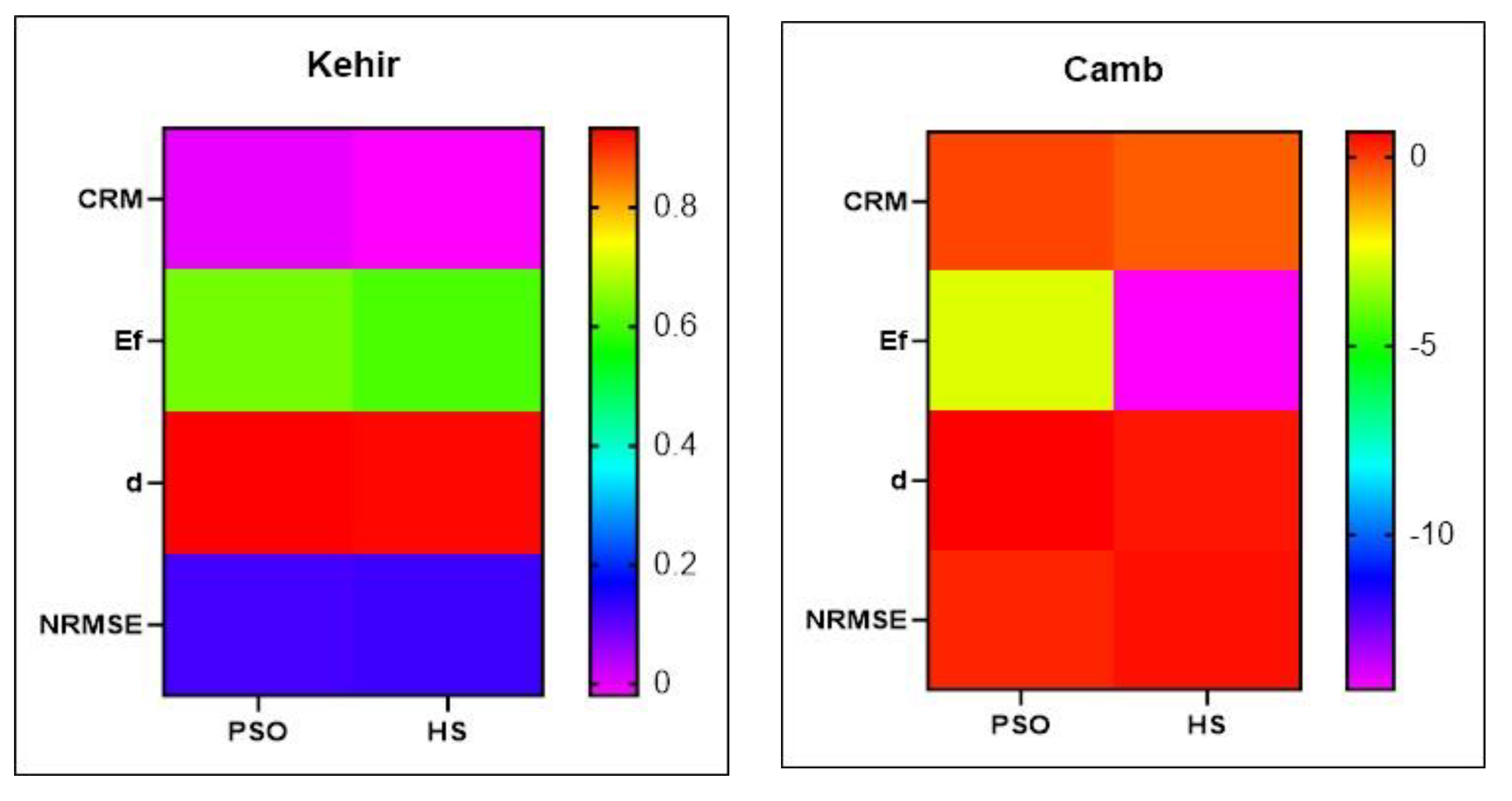
Heat maps in Figure 6 compare the performance of PSO and HS algorithms in optimizing the Muskingum-Cunge model coefficients at different stations based on CRM, Ef, d, and NRMSE indices. Brighter colors indicate better performance. Generally, PSO outperforms HS in terms of CRM, Ef, and NRMSE at most stations, suggesting its superiority in simulating flood hydrographs. However, there’s little difference between the two algorithms in terms of the ‘d’ index. At stations like Kajo, NikShahr, Rapch, Sarbaz, Siyah Jangal, and Kahir, PSO consistently provides more accurate simulations. At Kamb, PSO significantly outperforms HS across all indices, particularly in terms of Ef (PSO: -2.69 vs HS: -14.10) and NRMSE (PSO: 0.24 vs HS: 0.49). The performance difference is most pronounced at this station, with PSO showing markedly better results in simulating flood hydrographs.

Table 3. presents statistical analysis results for four indices (CRM, Ef, d, NRMSE) comparing PSO and HS models at various stations. PSO consistently performed as well or better than HS across all locations. Notably, PSO significantly outperformed HS at Bahu and Kamb stations, with substantial improvements in Ef and CRM indices. While both models performed well at Siyah Jangal, PSO showed marginally better results. At Kajo and NikShahr, PSO demonstrated moderate performance advantages across the indices

5. Conclusion

This study compared the performance of Particle Swarm Optimization (PSO) and Harmony Search (HS) algorithms in optimizing Muskingum-Cunge model parameters for flood routing across multiple stations. Results consistently demonstrated PSO’s superiority over HS in simulating flood hydrographs. While both algorithms achieved acceptable accuracy at most stations, as evidenced by correlation coefficients ranging from 0.6558 to 0.9645, PSO exhibited consistently better performance across various evaluation metrics (CRM, Ef, NRMSE). This superiority was particularly pronounced at stations with complex hydrological conditions, such as Bahu and Kamb. Both PSO and HS effectively optimized Muskingum-Cunge model parameters, leading to accurate simulations of flood outflow discharge. However, PSO’s ability to explore the solution space more efficiently resulted in superior parameter estimates and consequently improved hydrograph predictions. Heat map analysis and statistical comparisons further reinforced PSO’s dominance. While both algorithms captured the general trends in flood hydrographs, PSO exhibited a more precise representation of peak flows and hydrograph shapes.While both PSO and HS are valuable tools for flood modeling, the findings of this study strongly advocate for PSO as the preferred optimization algorithm for the Muskingum-Cunge model. Future research should focus on understanding the underlying reasons for PSO’s superior performance and exploring hybrid approaches that combine the strengths of both algorithms.

References

Lama, G.F.C.; Rillo Migliorini Giovannini, M.; Errico, A.; Mirzaei, S.; Padulano, R.; Chirico, G.B.; Preti, F. Hydraulic efficiency of green-blue flood control scenarios for vegetated rivers: 1D and 2D unsteady simulations. Water 2021, 13, 2620. [Google Scholar] [CrossRef]
Mel, R.A.; Viero, D.P.; Carniello, L.; D’Alpaos, L. Optimal floodgate operation for river flood management: The case study of Padova (Italy). Journal of Hydrology: Regional Studies 2020, 30, 100702. [Google Scholar] [CrossRef]
Pinter, N.; Heine, R.A. Hydrodynamic and morphodynamic response to river engineering documented by fixed-discharge analysis, Lower Missouri River, USA. Journal of Hydrology 2005, 302, 70–91. [Google Scholar] [CrossRef]
Gaagai, A.; Aouissi, H.A.; Krauklis, A.E.; Burlakovs, J.; Athamena, A.; Zekker, I.; Boudoukha, A.; Benaabidate, L.; Chenchouni, H. Modeling and risk analysis of dam-break flooding in a semi-arid Montane watershed: a case study of the Yabous Dam, Northeastern Algeria. Water 2022, 14, 767. [Google Scholar] [CrossRef]
Herrera-Granados, O. Theoretical background and application of numerical modeling to surface water resources. In Current Directions in Water Scarcity Research; Elsevier: 2022; Volume 7, pp. 319–340.
Zafar, M.B. Analysis of Channel and Floodplain Hydrodynamics and Flooding on the Mississippi River; Michigan State University: 2023.
Grimaldi, S.; Schumann, G.P.; Shokri, A.; Walker, J.; Pauwels, V. Challenges, opportunities, and pitfalls for global coupled hydrologic-hydraulic modeling of floods. Water Resources Research 2019, 55, 5277–5300. [Google Scholar] [CrossRef]
Jain, S.K.; Mani, P.; Jain, S.K.; Prakash, P.; Singh, V.P.; Tullos, D.; Kumar, S.; Agarwal, S.P.; Dimri, A.P. A Brief review of flood forecasting techniques and their applications. International journal of river basin management 2018, 16, 329–344. [Google Scholar] [CrossRef]
Roohi, M.; Soleymani, K.; Salimi, M.; Heidari, M. Numerical evaluation of the general flow hydraulics and estimation of the river plain by solving the Saint–Venant equation. Modeling Earth Systems and Environment 2020, 6, 645–658. [Google Scholar] [CrossRef]
Tsai, C.W. Applicability of kinematic, noninertia, and quasi-steady dynamic wave models to unsteady flow routing. Journal of Hydraulic Engineering 2003, 129, 613–627. [Google Scholar] [CrossRef]
Ehteram, M.; Shabanian, H. Unveiling the SALSTM-M5T model and its python implementation for precise solar radiation prediction. Energy Reports 2023, 10, 3402–3417. [Google Scholar] [CrossRef]
Moradi, E.; Yaghoubi, B.; Shabanlou, S. A new technique for flood routing by nonlinear Muskingum model and artificial gorilla troops algorithm. Applied Water Science 2023, 13, 49. [Google Scholar] [CrossRef]
Bozorg-Haddad, O.; Mohammad-Azari, S.; Hamedi, F.; Pazoki, M.; Loáiciga, H.A. Application of a new hybrid non-linear Muskingum model to flood routing. In Proceedings of the Proceedings of the institution of civil engineers-water management, 2020; pp. 109–120.
Akbari, R.; Hessami-Kermani, M.-R.; Shojaee, S. Flood routing: improving outflow using a new non-linear Muskingum model with four variable parameters coupled with PSO-GA algorithm. Water Resources Management 2020, 34, 3291–3316. [Google Scholar] [CrossRef]
Bozorg-Haddad, O.; Abdi-Dehkordi, M.; Hamedi, F.; Pazoki, M.; Loáiciga, H.A. Generalized storage equations for flood routing with nonlinear Muskingum models. Water Resources Management 2019, 33, 2677–2691. [Google Scholar] [CrossRef]
Das, A. Parameter estimation for Muskingum models. Journal of Irrigation and Drainage Engineering 2004, 130, 140–147. [Google Scholar] [CrossRef]
Karahan, H.; Gurarslan, G.; Geem, Z.W. A new nonlinear Muskingum flood routing model incorporating lateral flow. Engineering Optimization 2015, 47, 737–749. [Google Scholar] [CrossRef]
Norouzi, H.; Bazargan, J. Using the linear muskingum method and the particle swarm optimization (PSO) algorithm for calculating the depth of the rivers flood. Iran-Water Resources Research 2019, 15, 344–347. [Google Scholar]
Niazkar, M.; Afzali, S.H. New nonlinear variable-parameter Muskingum models. KSCE Journal of Civil Engineering 2017, 21, 2958–2967. [Google Scholar] [CrossRef]
Gąsiorowski, D.; Szymkiewicz, R. Identification of parameters influencing the accuracy of the solution of the nonlinear Muskingum equation. Water Resources Management 2020, 34, 3147–3164. [Google Scholar] [CrossRef]
Soltani, S.R.K.; Mostafaeipour, A.; Almutairi, K.; Dehshiri, S.J.H.; Dehshiri, S.S.H.; Techato, K. Predicting effect of floating photovoltaic power plant on water loss through surface evaporation for wastewater pond using artificial intelligence: A case study. Sustainable Energy Technologies and Assessments 2022, 50, 101849. [Google Scholar] [CrossRef]
Prawira, D.; Soeryantono, H.; Anggraheni, E.; Sutjiningsih, D. Efficiency analysis of Muskingum-Cunge method and kinematic wave method on the stream routing (Study case: upper Ciliwung watershed, Indonesia). In Proceedings of the IOP Conference Series: Materials Science and Engineering; 2019; p. 012036. [Google Scholar]
Ehteram, M.; Binti Othman, F.; Mundher Yaseen, Z.; Abdulmohsin Afan, H.; Falah Allawi, M.; Bt. Abdul Malek, M.; Najah Ahmed, A.; Shahid, S.; P. Singh, V.; El-Shafie, A. Improving the Muskingum flood routing method using a hybrid of particle swarm optimization and bat algorithm. Water 2018, 10, 807. [Google Scholar] [CrossRef]
Piri, J.; Mollaeinia, M.; Mostafaie, A. Assessment of response surface method and hybrid models to predict evaporation (case study: Chahnimeh and Pishein reservoirs in Sistan and Baluchestan Province of Iran). Arabian Journal of Geosciences 2023, 16, 346. [Google Scholar] [CrossRef]
Kennedy, J.; Eberhart, R. Particle swarm optimization. In Proceedings of the Proceedings of ICNN’95-international conference on neural networks, 1995; pp. 1942–1948.
Shi, Y.; Eberhart, R. A modified particle swarm optimizer. In Proceedings of the 1998 IEEE international conference on evolutionary computation proceedings. IEEE world congress on computational intelligence (Cat. No. 98TH8360); 1998; pp. 69–73. [Google Scholar]
Eberhart, R.C.; Shi, Y.; Kennedy, J. Swarm intelligence; Elsevier: 2001.
Jabari, F.; Mohammadnejad, J.; Yavari, K. Human primary dental pulp mesenchymal stem cells: History and isolation methods. Journal of Dental Medicine 2014, 27, 184–189. [Google Scholar]
Geem, Z.W.; Kim, J.H.; Loganathan, G.V. A new heuristic optimization algorithm: harmony search. simulation 2001, 76, 60–68. [Google Scholar] [CrossRef]
Jahantigh, N.; Piri, J. Estimation of solar radiation in different climates of Iran using hybrid machine learning methods. 2023.
Lees, T. Deep learning for hydrological modelling: from benchmarking to concept formation. University of Oxford, 2022.
McCuen, R.H.; Knight, Z.; Cutter, A.G. Evaluation of the Nash–Sutcliffe efficiency index. Journal of hydrologic engineering 2006, 11, 597–602. [Google Scholar] [CrossRef]
Piri, J.; Abdolahipour, M.; Keshtegar, B. Advanced machine learning model for prediction of drought indices using hybrid SVR-RSM. Water Resources Management 2023, 37, 683–712. [Google Scholar] [CrossRef]
Moriasi, D.N.; Arnold, J.G.; Van Liew, M.W.; Bingner, R.L.; Harmel, R.D.; Veith, T.L. Model evaluation guidelines for systematic quantification of accuracy in watershed simulations. Transactions of the ASABE 2007, 50, 885–900. [Google Scholar] [CrossRef]

Figure 1. Study area and river basins in Baluchistan.

Figure 2. Flowchart of particle swarm optimization algorithm (PSO).

Figure 3. Flowchart of Harmony Search Algorithm (HS).

Figure 4. Comparing the results of PSO and HS models of the optimization of Muskingum Kange coefficients against the actual flood flow for stations.

Figure 5. Chart of inlet flow and outlet flow with PSO and HS models, optimization of Muskingum Kange coefficients for Kajo station.

Figure 6. Heat map to compare statistical results in stations.

Table 1. Characteristics of the studied rivers and basins in Baluchestan.

No.	River Name	Length (m)	Perimeter (km)	Area (km²)	City
1	Rapch	23,000	897.1	7944	Konarak
2	Kajou	34500	838	6717	Qasr-e Qand
3	Bahu	9860	189.4	987	Chabahar
4	Nikshahr	18500	142.3	373.4	Nikshahr
5	Kehir	20546	354.2	3004	Nikshahr
6	Sarbaz	56000	764.3	6850	Sarbaz
7	Kamb	21300	208	130	Chabahar
8	Siah Jangal	24756	254.2	1350	Mirjaveh

Table 2. Initial estimates for parameters X and K were obtained using Particle PSO and HS algorithms.

No.	River Name	PSO		HS
		x	K	x	K
1.00	Rapch	0.29	24.40	0.24	25.12
2.00	Kajou	0.41	24.80	0.35	21.40
3.00	Bahu	0.16	15.91	0.17	16.02
4.00	Nikshahr	0.24	8.42	0.25	8.56
5.00	Kehir	0.24	29.11	0.23	28.60
6.00	Sarbaz	0.23	8.60	0.25	8.74
7.00	Kamb	0.18	2.90	0.19	2.85
8.00	Siah Jangal	0.42	6.40	0.43	6.21

Table 3. Results of statistical analysis for stations.

Station		PSO	HS
Kajo	CRM	0.02	0.01
	Ef	0.92	0.92
	d	0.98	0.98
	NRMSE	0.10	0.10
Bahu	CRM	-0.04	-0.12
	Ef	-1.97	-3.82
	d	0.73	0.64
	NRMSE	0.17	0.22
NikShahr	CRM	-0.03	-0.09
	Ef	0.39	0.03
	d	0.89	0.85
	NRMSE	0.14	0.17
Rapch	CRM	-0.03	-0.06
	Ef	0.43	0.32
	d	0.90	0.88
	NRMSE	0.15	0.16
Sarbaz	CRM	0.00	-0.03
	Ef	0.35	0.25
	d	0.89	0.88
	NRMSE	0.14	0.15
Siyah Jangal	CRM	-0.01	-0.02
	Ef	0.94	0.94
	d	0.99	0.99
	NRMSE	0.08	0.09
Kahir	CRM	-0.01	-0.02
	Ef	0.64	0.61
	d	0.93	0.93
	NRMSE	0.12	0.13
Kamb	CRM	-0.13	-0.41
	Ef	-2.69	-14.10
	d	0.67	0.42
	NRMSE	0.24	0.49

Disclaimer/Publisher’s Note: The statements, opinions and data contained in all publications are solely those of the individual author(s) and contributor(s) and not of MDPI and/or the editor(s). MDPI and/or the editor(s) disclaim responsibility for any injury to people or property resulting from any ideas, methods, instructions or products referred to in the content.

© 2024 by the authors. Licensee MDPI, Basel, Switzerland. This article is an open access article distributed under the terms and conditions of the Creative Commons Attribution (CC BY) license (http://creativecommons.org/licenses/by/4.0/).

Copyright: This open access article is published under a Creative Commons CC BY 4.0 license, which permit the free download, distribution, and reuse, provided that the author and preprint are cited in any reuse.

MDPI Initiatives

Important Links

Choose an area of interest and we will send you notifications of new preprints at your preferred frequency.

Disclaimer