1. Introduction
Over the past decade, there has been an intense debate surrounding the issue of Moore’s Law reaching its limits. This law postulates that the number of transistors in an integrated circuit doubles at nearly regular intervals. With the development of nanometer-scale technology, standard CMOS technology has reached its scalability limits. Consequently, there is a need to find solutions that would increase both the performance of modern computers and the amount of available memory. One such idea is to shift from the classic von Neumann architecture, where the processor and memory are separated by a data bus, to an integrated architecture known as in-memory computing. Another idea is to replace the bi-stable transistor with a multi-stable element. With the emergence of actual memristive devices, both of these ideas seem feasible.
Following Professor Leon Chua’s postulation of the memristor in 1971 [
1], it took another 37 years for the physical implementation of this element to be achieved. In 2008, the HP Labs team led by R. Stanley Williams published their work on creating a memristor based on titanium dioxide (
) [
2]. Since then, numerous other memristor designs have emerged, differing in their structure, materials, and operating principles e.g. polymers memristors [
3,
4], ferroelectric memristors [
5], spintronic memristors [
6,
7,
8]. One of the most intriguing types of memristors are the Self Directed Channel (SDC) memristors produced by Knowm Inc. They have been described in numerous publications [
9,
10,
11].
Realizing the multitude of memristor designs available today, in the design of each prototype circuit, a crucial aspect is simulating the behavior of the circuit under various stimuli. Therefore, it is essential to faithfully replicate the dynamics of memristive elements using their model. This paper will analyze which model best reproduces the behavior of SDC memristors and develop an algorithm to optimize model parameters based on real measurement data. Optimized parameters can be successfully applied in simulation environments such as SPICE or Simulink.
The paper discusses the optimization of parameters for various models based on real measurement data of SDC memristors with different dopings, namely tungsten, tin, chromium, and carbon, using two algorithms: SQP and Nelder-Mead. Box constraints were imposed on individual parameters during optimization. Since in the paper [
12], Strukov, Assymetric Strukov and VTEAM models were compared, it was decided to compare other models with the most accurate model from this work, namely the VTEAM model.
2. Materials and Methods
The SDC memristors with tungsten W, carbon C, tin Sn and chromium Cr doping were subjected to research and measurements.
To measure the current of the memristor and limit it below the nominal value, i.e., 1 mA for memristors doped with
and 50
for doping with
[
10], the memristor was connected in series with a linear resistor
. In the case of doping with
, the resistance
, while for doping with
,
. The voltage
measured across the resistor
which is a high-quality resistor utilized for accurately determining the memristor’s current, according to Ohm’s law, is directly proportional to the current and its known resistance, allowing the current of the memristor to be obtained by multiplying the voltage across the resistor by the reciprocal of its resistance. The schematic diagram of the measuring circuit is presented in
Figure 1a. Using
myDAQ University Kit device from National Instruments containing a measurement card and function generator, the supply voltage was generated and signals
and
were collected [
13]. The current and voltage of the memristor were calculated using Ohm’s law and Kirchhoff’s second law. The data acquisition and preliminary data processing process was written and implemented in the graphical programming environment
LabVIEW [
14,
15]. The utilized code is provided in the attached appendices. The circuit connection diagram to the measurement device is shown in
Figure 1b.
The voltage across the memristor were calculated using formula and the memristor current were calculated as .
Before starting measurements, it is necessary for the memristor to be formed. Forming is done by gradually increasing the voltage to create the necessary conductive paths inside the memristor. However, this voltage should not exceed the nominal operating voltage [
10,
12]. After forming the memristor, the circuit shown in
Figure 1 is powered by a sinusoidal alternating voltage
with amplitudes
and different frequencies, where
. Therefore, 18 tests were performed for one memristor, where each test consists of 100 periods and 1000 points for each period.
4. Optimization Procedure
In this section, the optimization procedure will be described, aimed at finding the optimal parameters for the models described in
Section 3.
The discussed optimization involves minimizing a certain objective function
F, which is tasked with comparing the waveform of the model function with the actual waveform of the memristor. The requirement is for the function to decrease as the similarity between the resulting model and the estimated actual element waveform increases. The objective function used in this work is a modified coefficient of determination and is defined as [
20]:
Where
represents the model function,
and
denote the memristor voltage and current accordingly,
a is a
dimension vector of the real valued model parameters (
),
b is a
dimension vector of integer valued model parameters (
), RSS denotes the residual sum of squares, and TSS is the total sum of squares. The functions RSS and TSS take the following form:
The parameters are:
, which represents the actual value of the
i-th sample,
, denoting the value predicted by the model,
n, representing the number of samples in the period, and
, which is the average value of the samples in the period. The reference values of the memristor current and voltage come from the determined averaged periods of the signal.
During optimization, appropriate values of parameters collected in vectors
a and
b need to be found so that the objective function reaches its minimum. These parameters can be defined as real or natural numbers, depending on the specific model. For parameters that should be natural numbers, the optimization process is performed using the brute force method, i.e., for each combination within a specified range, and then the ones for which the objective function is the lowest are selected. This algorithm significantly prolongs the optimization time. Parameters that should be natural numbers are the parameters
and
in the VTEAM model. Floating-point parameters are also subject to certain constraints, mainly due to the nature of the model. Because the input signal to the system is a continuous sinusoidal function, it is necessary to ensure that the response signal is also a continuous and periodic function. This is ensured when the internal variable of the memristor
x is also a continuous and periodic function, so
, where
T is the period, indicating that the system is in a steady state. This condition requires optimizing an additional parameter,
, which is a constant of integration when integrating the internal variable function and represents the value of the internal variable at the time
of measurement. To ensure the continuity condition, an algorithm is proposed consisting of preliminary optimization of the objective function described by equation (
14), followed by optimization of a new objective function, which rewards for the continuity and periodicity of the internal variable function, as proposed (
17):
Parameters
w,
, and
are elements of the optimization algorithm. Parameter
w is a weight chosen according to the continuity of the function. Parameters
and
are, respectively, the first and last elements of the internal variable function. If the condition
is met, the algorithm terminates its operation; otherwise, the optimization process of function (
17) is repeated for
until the condition is satisfied. To increase the number of reference points and reduce the integration step, the interpolation method called
Akima Spline [
21] is utilized, which performs local fitting of the function, and the number of points is increased tenfold. The optimization process for the mentioned models differs slightly. It should be noted that the obtained minima of the objective function may be only local minima, and there may be parameters for which the objective function can be even lower. Optimization methods are listed in the subsequent subsections.
4.1. MMS Model
Optimization was performed based on six degrees of freedom represented by real valued parameters only:
and
. Two algorithms were utilized in the optimization process. The first one is the
SQP algorithm implemented in the
fmincon function of MATLAB [
22,
23,
24]. The
SQP method solves a sequence of sub-problems optimizing the quadratic objective model subject to linearized constraints. It ensures box constraints in all iterations and is resilient to objective function results such as
Nan and
Inf. It has many advantages, including low memory consumption and the ability to quickly solve problems. However, the solution may be inaccurate due to the barrier function maintaining parameters away from the box constraints [
23,
24] and when the algorithm stacks in the local minima. The second algorithm is the
Nelder-Mead algorithm, also known as the simplex downhill method. This algorithm does not use the gradient of the objective function [
25,
26]. It was implemented in the
fminsearch function of MATLAB; however, the optimization process utilized the
minimize function, which is available in the MATLAB external repository [
27]. Unlike the
fminsearch function, it allows for the introduction of box constraints within which parameters can change.
The optimization process involves initially minimizing the objective function (
14) using both algorithms, selecting parameters with the lowest value of this function, then minimizing the function (
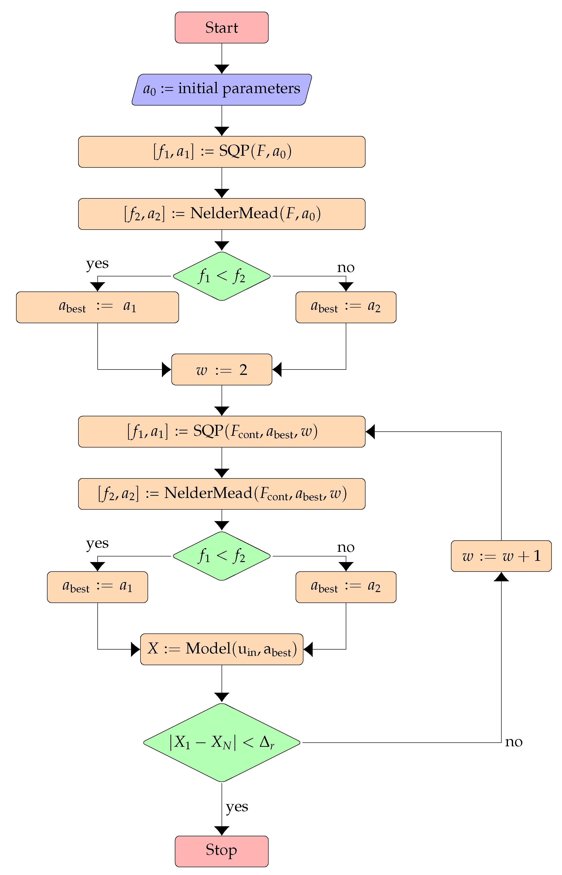
17) using both algorithms, with parameters obtained in the first stage of minimization, and finally selecting parameters for which the objective function value is the smallest, while simultaneously checking whether the internal variable of the function remains continuous and periodic. A simplified block diagram of the optimization algorithm is shown in
Figure 2. Box constraints for individual parameters are presented in
Table 1.
For the simulation and integration of the MMS model, the Runge-Kutta method called
,,RK4” was implemented independently in MATLAB [
17,
28]. To ensure that the model represents the parameters of a memristor, and not a memristor-linear resistor circuit, the first step is to calculate the value of the internal variable. Subsequently, using the fact that the relationship
is a linear, the memristor conductance can be calculated, as in equation (
6). The voltage is then calculated using a voltage divider
where
represent resistance of the series resistor. Subsequently, the memristor current is the product of the voltage
and the conductance
.
4.2. VTEAM Model
The optimization was conducted based on nine degrees of freedom, which are:
, and
. All these parameters are floating-point numbers, except for
and
, which should be natural numbers. The optimization process occurs just as for the MMS model described in
subsection 4.1, except that the optimization process takes place for each combination of the integer pair
and
, and then parameters are chosen for the smallest objective function. To limit the dimension of the integer space of the possible solutions the parameters
and
are chosen to be less then 10. Therefore, for a single test, for each amplitude of the driving signal and for each frequency, it was necessary to perform as many as 81 iterations. Additionally, the model employs the Biolek’s window function [
29] with parameter
p: for
, i.e., for the range
, and for
, i.e.,
[
19]. In the model,
and
is set so that the internal variable
x could change within a relative range from 0 to 1. The constraints for the optimization parameters are presented in the
Table 2.
4.3. Yakopcic Model
The optimization was performed based on twelve degrees of freedom. All the parameters are real. The optimization process is similar to that for the MMS and VTEAM models described in
subsection 4.1. However, the system modeled is as ,,memristor-linear resistor” due to the nonlinear relationship between the memristor current
and its voltage
, as shown in equation (
7). In this equation, it is challenging to directly obtain conductance or resistance since the voltage is an argument of the
function. The box constrains for each variable used in the optimization are provided in
Table 3.
7. Conclusions
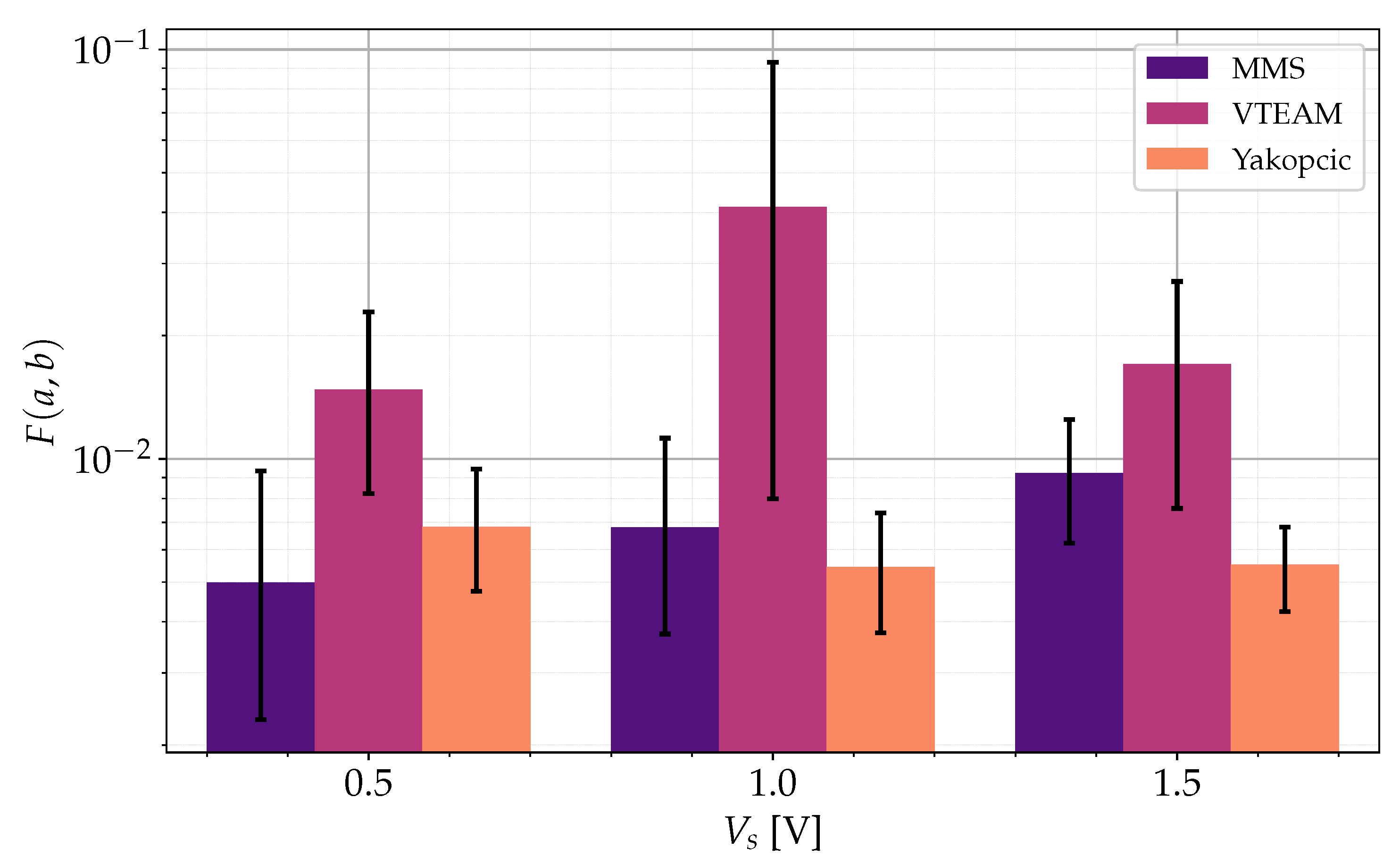
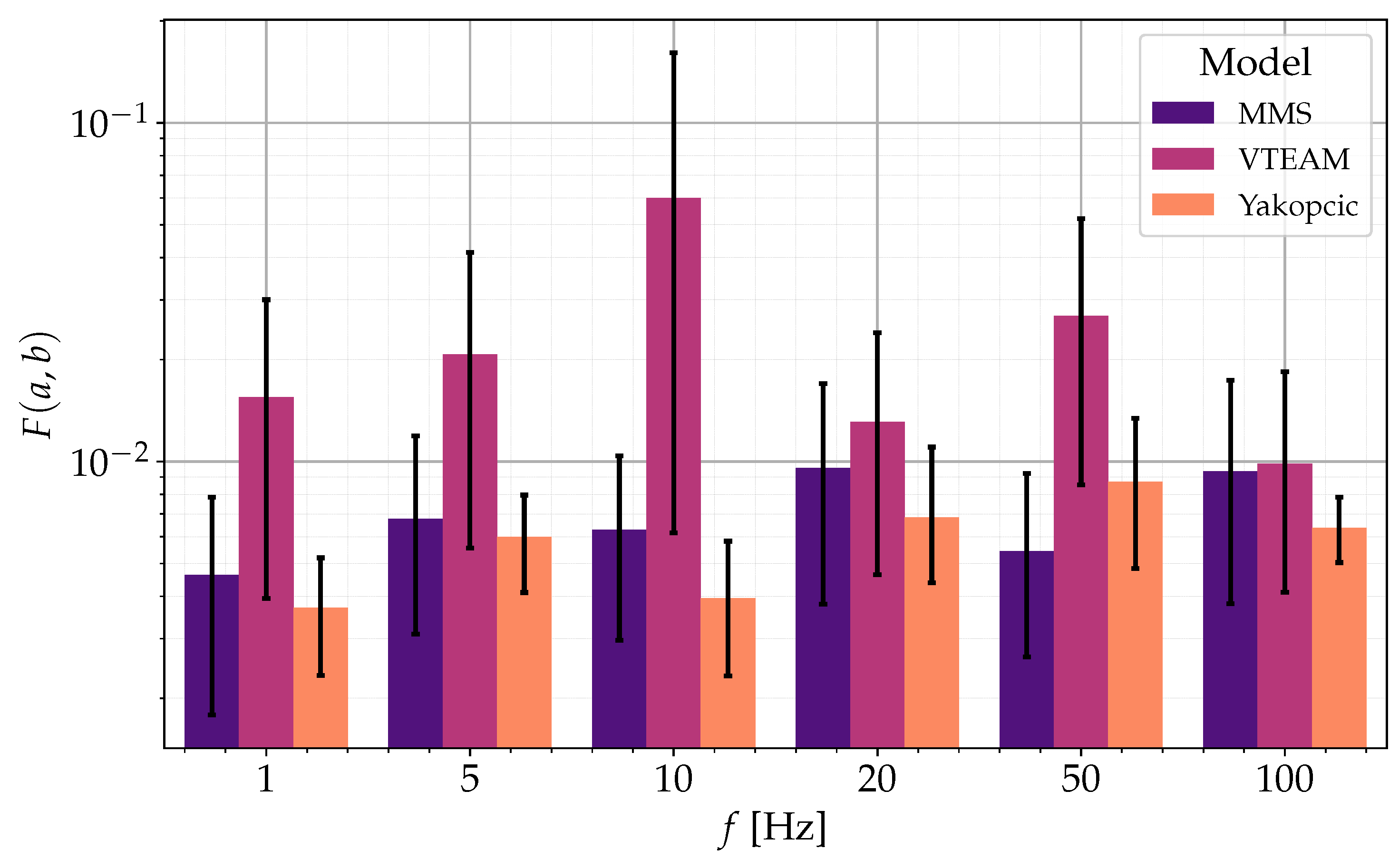
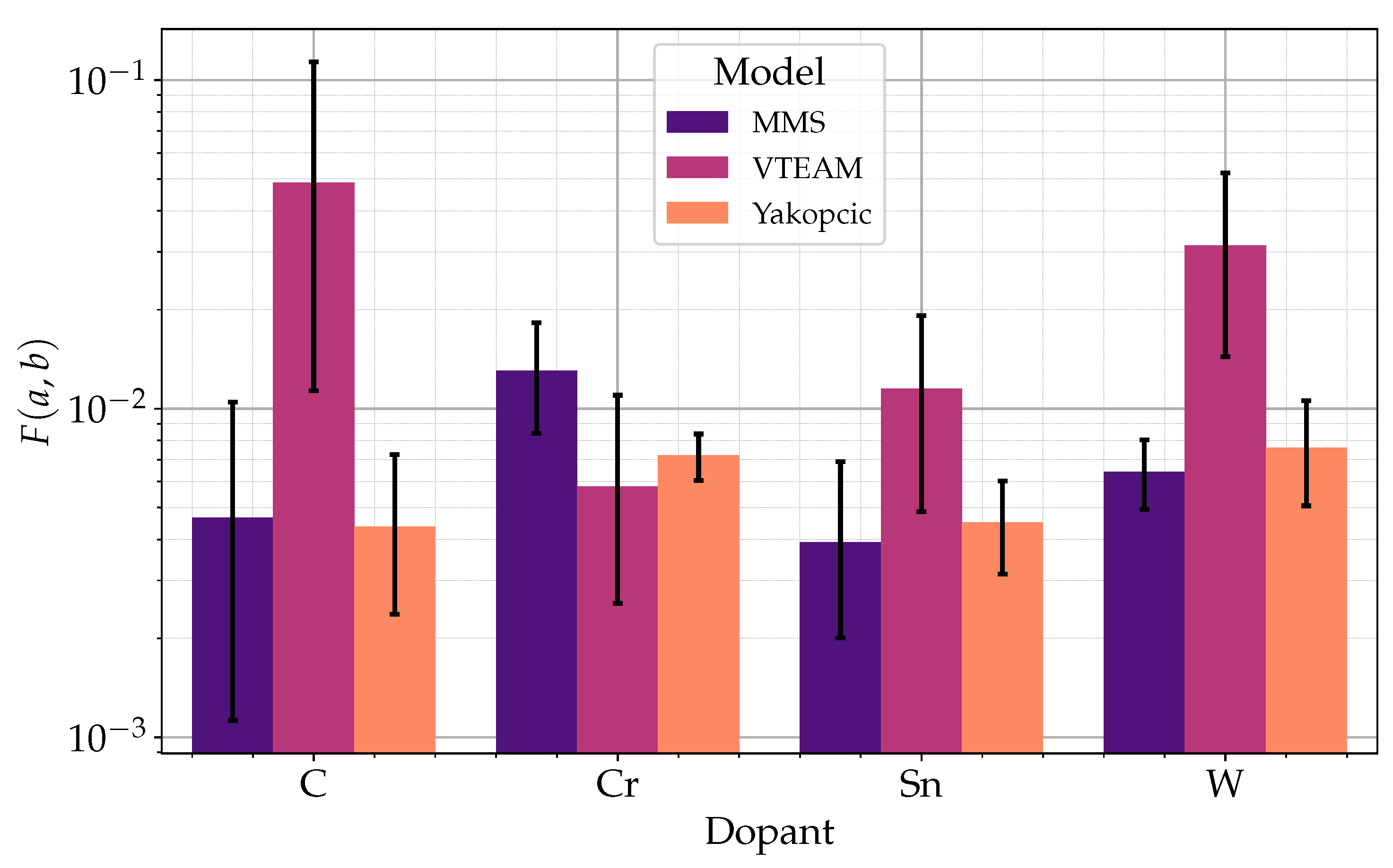
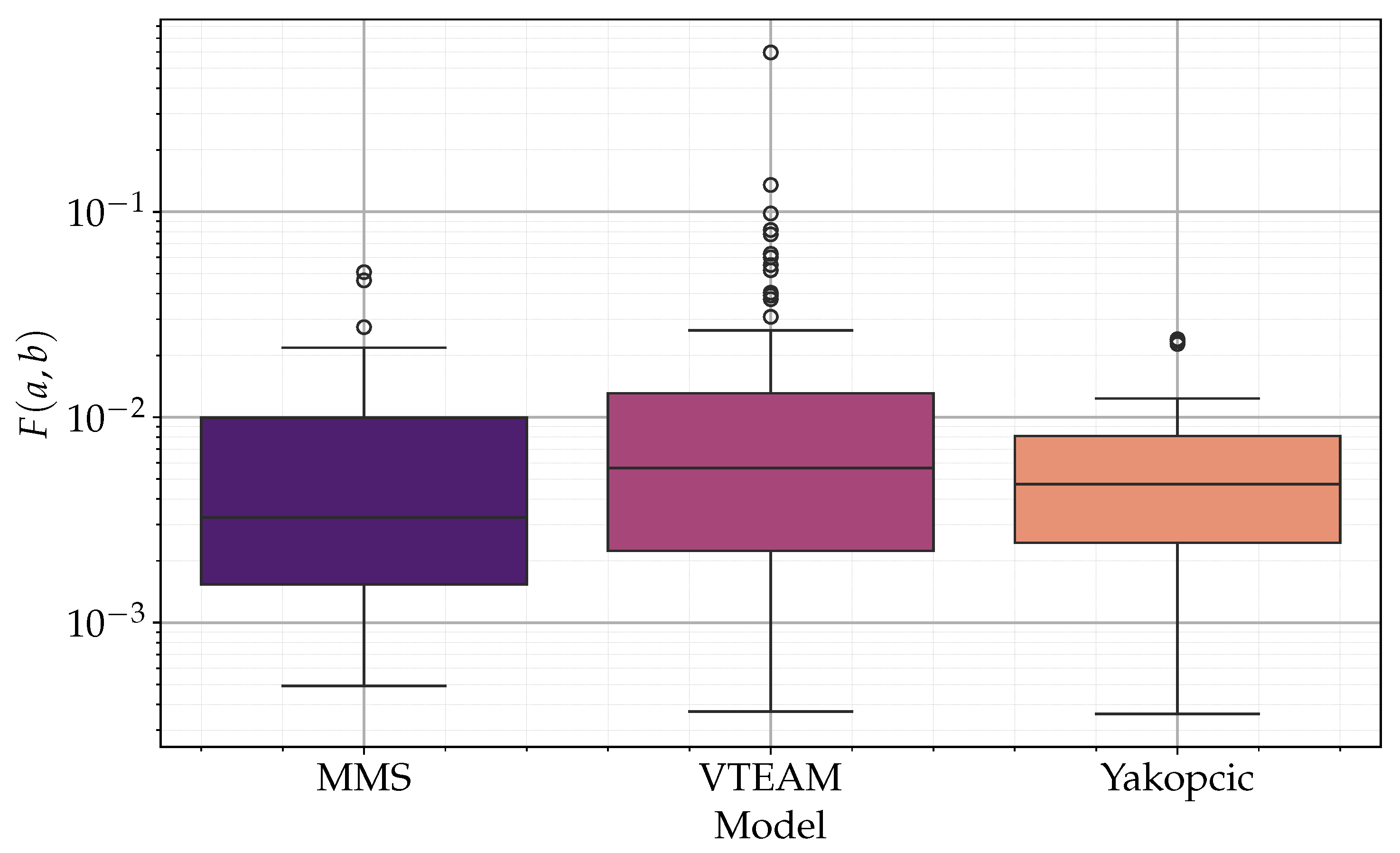
From the conducted optimizations, it can be concluded that they were successful, and the obtained objective functions achieved relatively low values. It can also be inferred that the best models for modeling SDC memristors are the MMS and Yakopcic models. They have similar low average values of the objective function, and the dispersion of these values is not large depending on the amplitude of the supply voltage, frequency, or type of doping. Definitely, compared to the models mentioned earlier, the worst model for optimization is the VTEAM model. It has the highest average values of the objective function and the largest dispersion. Taking into account the specifics of the model, especially the fact that natural parameters are required, the optimization of this model is quite tedious due to iterating over all possible combinations of integer parameters in the interval and selecting the best solution. This means that the time needed to minimize the objective function is several dozen times longer than the time needed for the MMS model. An additional problem is the undefined values by the objective function, which the minimizing algorithm must be resistant to. Taking into account also the specifics of individual models, it can be reflected that the MMS model is best suited for modeling SDC memristors due to its simplicity (only 6 degrees of freedom), linear dependence of current on voltage, and the fact that it does not have threshold ranges, so the function of the internal variable is monotonically continuous. The MMS model also has a physical interpretation in real memristors. The Yakopcic model was created to fit every type of memristor, and in the discussed case, quite good fits and low objective functions were obtained. However, it is quite complicated and does not have a linear dependence of current on voltage. Additionally, it is a mathematical concept and does not have a physical interpretation.
From the optimization results, it can also be concluded that the lowest objective functions are obtained for quite rounded waveforms where there is no sudden switching between states, which is called soft-switching [
17]. It occurs when the function of the internal variable
x does not reach the upper value of the range in which it is contained. This is especially visible when powered by signals with high frequency and low amplitude, as the energy and charge in each half-period are low and do not allow reaching the limit ranges of the internal variable. During the measurements the influence of the memristor’s temperature change has been noticed. In the future Authors consider to involve in the project of creating the optimal memristor model with temperature as additional parameter involved. The first idea seems to extend the MMS memristor model of this additional feature.
Figure 1.
The schematics of the measurement setup: (a) schematic diagram of the measurement circuit, (b) a simplified connection diagram of the measurement device to the circuit
Figure 1.
The schematics of the measurement setup: (a) schematic diagram of the measurement circuit, (b) a simplified connection diagram of the measurement device to the circuit
Figure 2.
Simplified block diagram of the optimization algorithm
Figure 2.
Simplified block diagram of the optimization algorithm
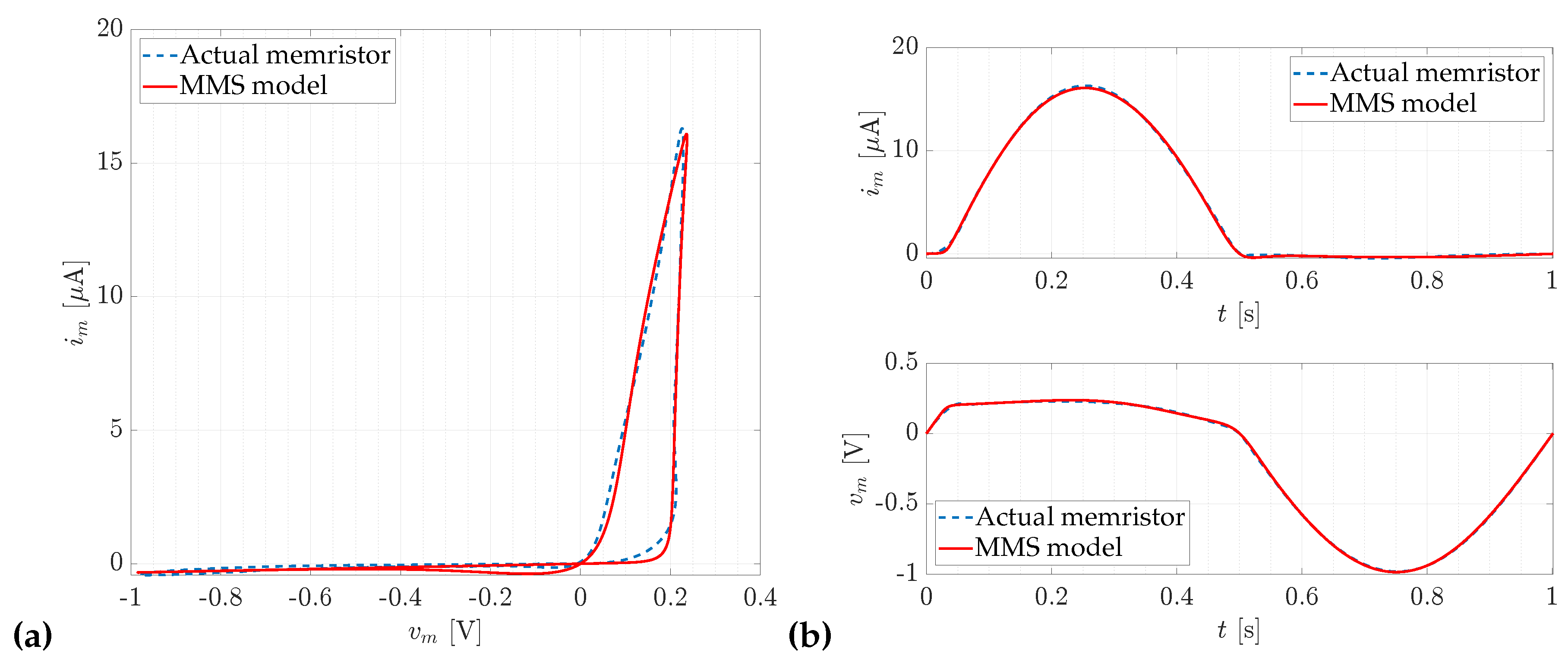
Figure 3.
The optimization results obtained for the MMS model with carbon doping, with a supply amplitude of and frequency , yield an objective function value for this case of . (a) Comparison of the hysteresis curves of the memristor , both the reference and the ones obtained during optimization. (b) Comparison of the currents and voltages of the memristor with those obtained as a result of model optimization.
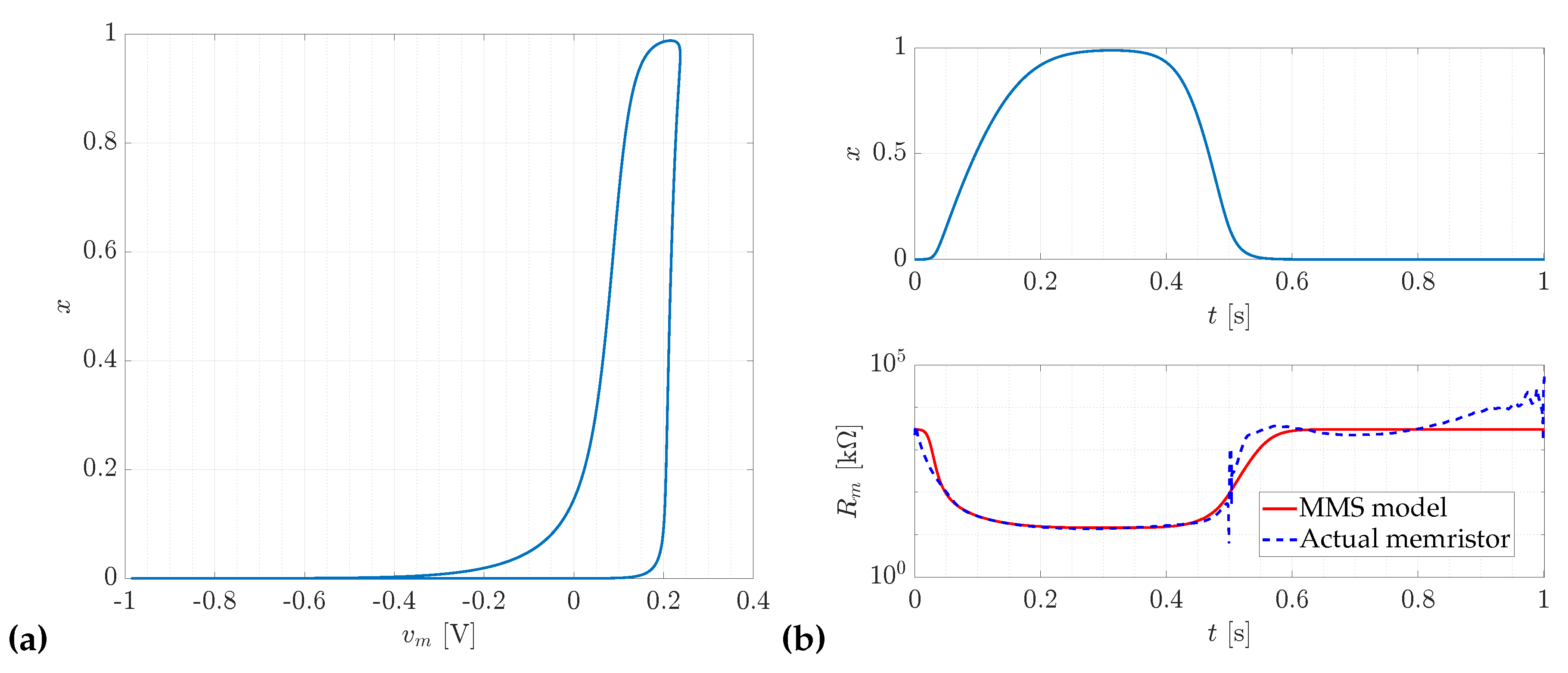
Figure 4.
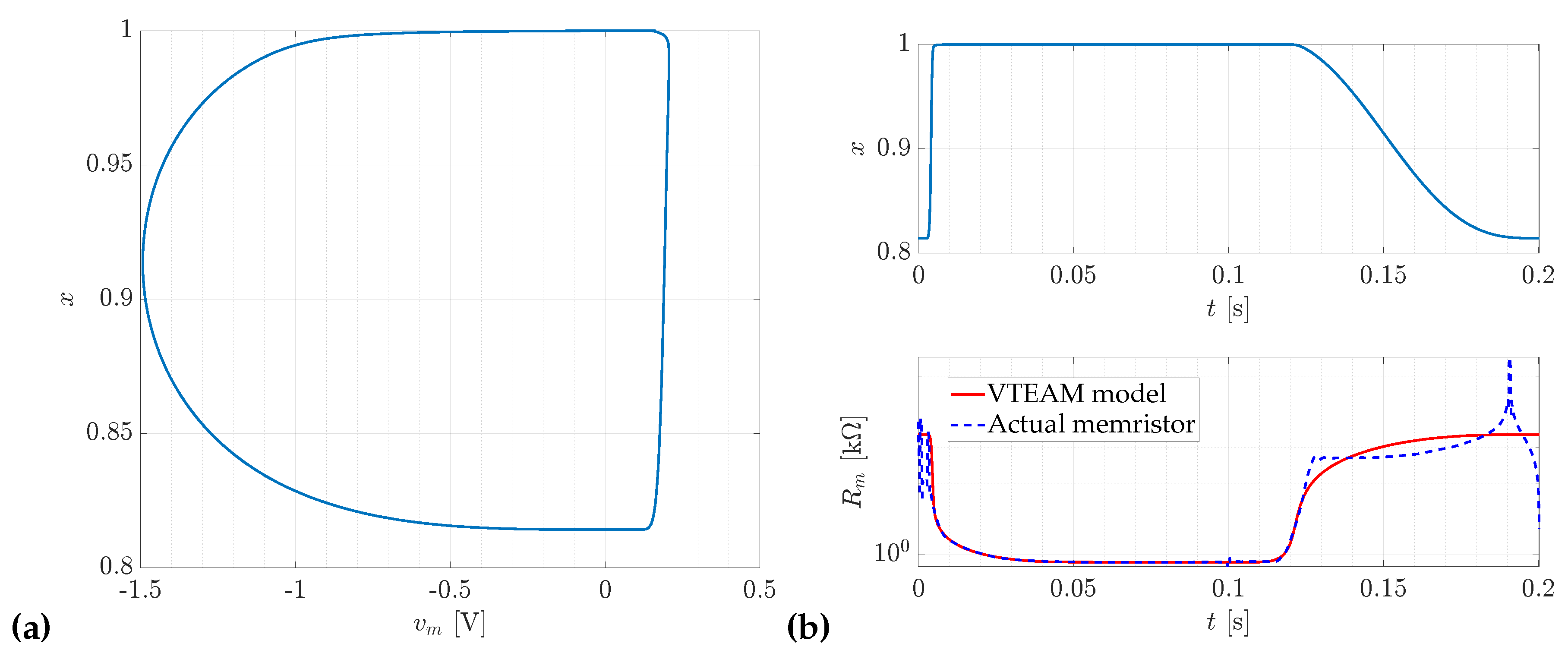
The profiles of the internal variable and resistance obtained for the MMS model with carbon doping, with a supply amplitude of and frequency , yield an objective function value for this case of . (a) The variation of the internal state variable x as a function of the memristor voltage .(b) The variation of the internal variable x and the memristor resistance over time.
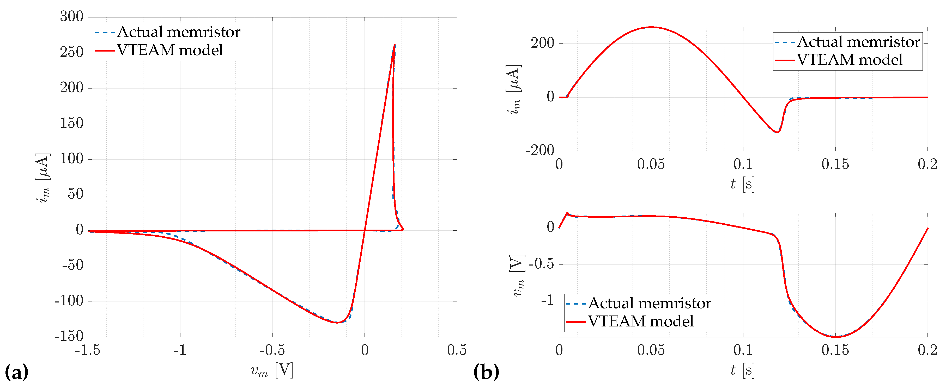
Figure 5.
The optimization results obtained for the VTEAM model with chromium doping, with a supply amplitude of and frequency , yield an objective function value for this case of . (a) Comparison of the hysteresis curves of the memristor , both the reference and the ones obtained during optimization. (b) Comparison of the currents and voltages of the memristor with those obtained as a result of model optimization.
Figure 6.
The optimization results obtained for the VTEAM model with chromium doping, with a supply amplitude of and frequency , yield an objective function value for this case of . (a) The variation of the internal state variable x as a function of the memristor voltage . (b) The variation of the internal variable x and the memristor resistance over time.
Figure 7.
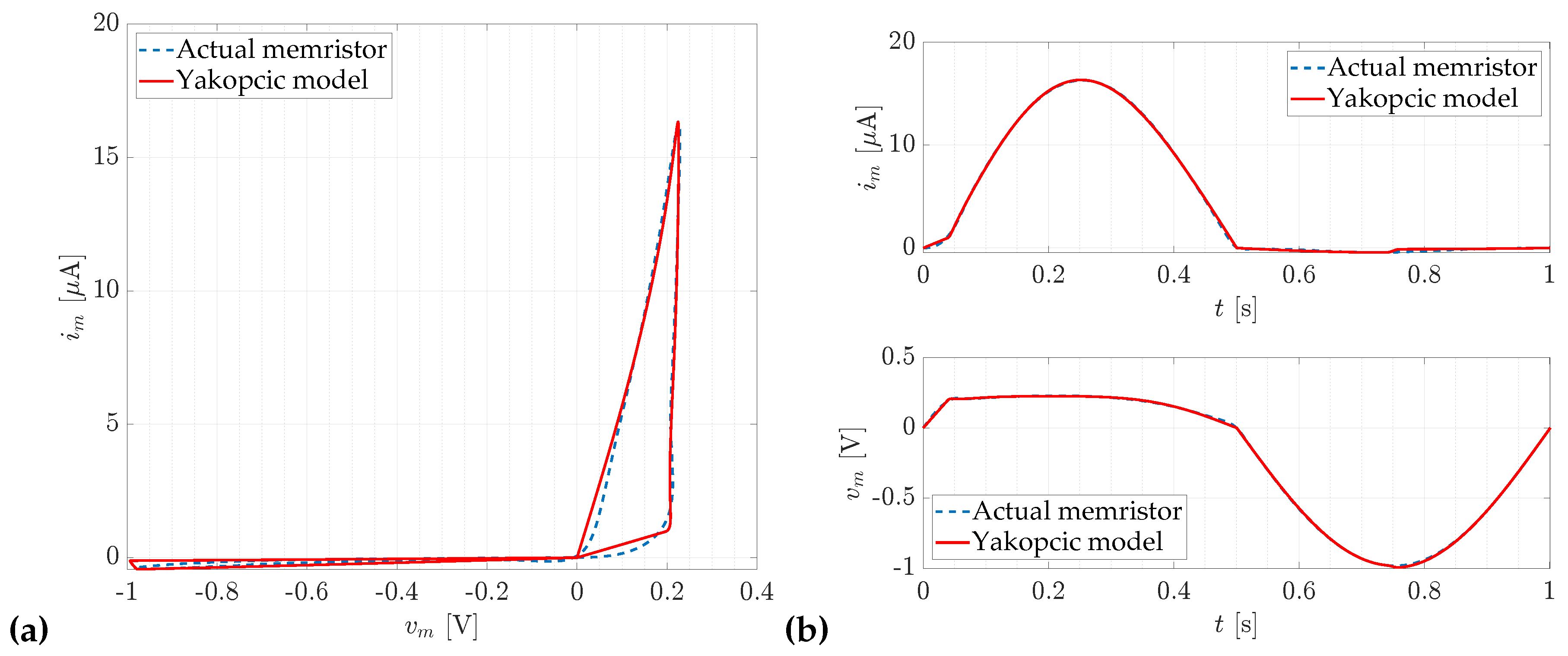
The optimization results obtained for the Yakopcic model with carbon doping, at a supply amplitude of and frequency , yield an objective function value of for this particular case. (a) Comparison of the hysteresis curves of the memristor , both the reference and the ones obtained during optimization. (b) Comparison of the currents and voltages of the memristor with those obtained as a result of model optimization.
Figure 8.
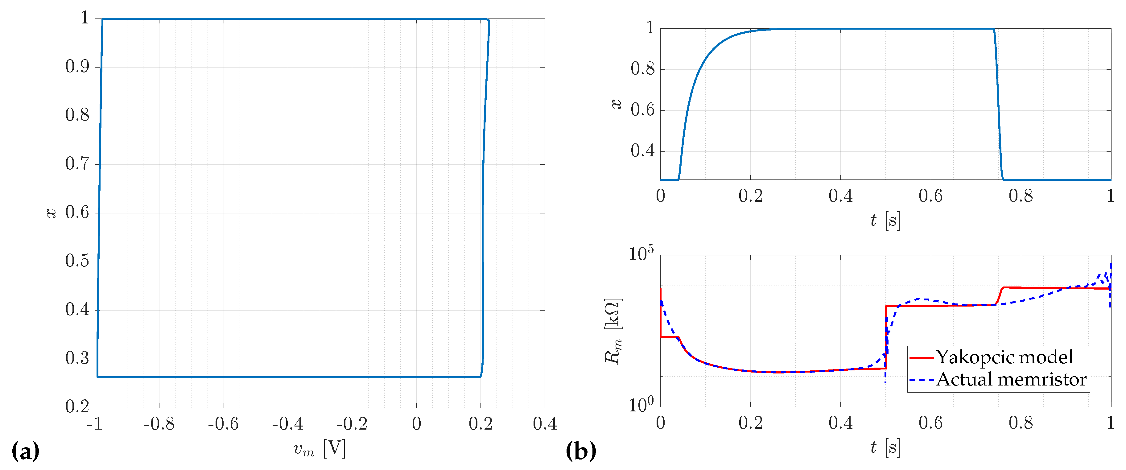
The trajectories of the internal state variable and resistance obtained for the Yakopcic model with carbon doping, at a supply amplitude of and frequency , yield an objective function value of for this particular case. (a) The variation of the internal state variable x as a function of the memristor voltage . (b) The variation of the internal variable x and the memristor resistance over time.
Figure 9.
The average objective function values for each model as a function of the supply voltage amplitude applied to the memristor-resistor system. The y-axis is presented on a logarithmic scale.
Figure 9.
The average objective function values for each model as a function of the supply voltage amplitude applied to the memristor-resistor system. The y-axis is presented on a logarithmic scale.
Figure 10.
The average objective function values for each model as a function of the frequency of the supply voltage applied to the memristor-resistor system. The y-axis is presented on a logarithmic scale.
Figure 10.
The average objective function values for each model as a function of the frequency of the supply voltage applied to the memristor-resistor system. The y-axis is presented on a logarithmic scale.
Figure 11.
The average objective function values for each model as a function of the memristor doping material. The y-axis is presented on a logarithmic scale.
Figure 11.
The average objective function values for each model as a function of the memristor doping material. The y-axis is presented on a logarithmic scale.
Figure 12.
Box plot of the objective function values for each model.
Figure 12.
Box plot of the objective function values for each model.
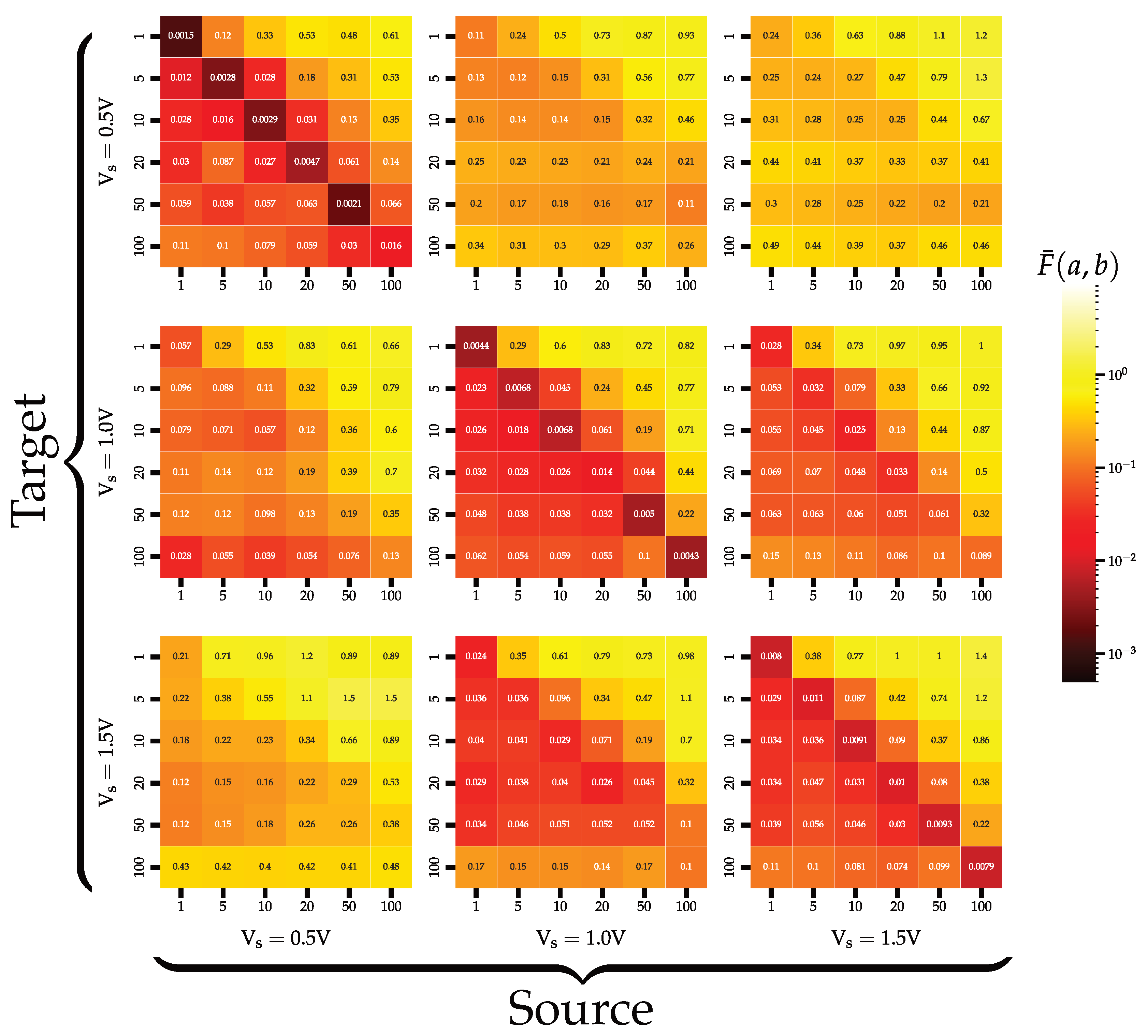
Figure 13.
An exemplary matrix in the form of a heatmap, where both color and annotation depict the value of the averaged objective function, is presented. On the left side of the graph are the excitation parameters for which the model was optimized, while along the bottom are the excitation parameters for which the model was evaluated. The graph contains data from the MMS model. For enhanced visibility, the color scale has been logarithmically adjusted.
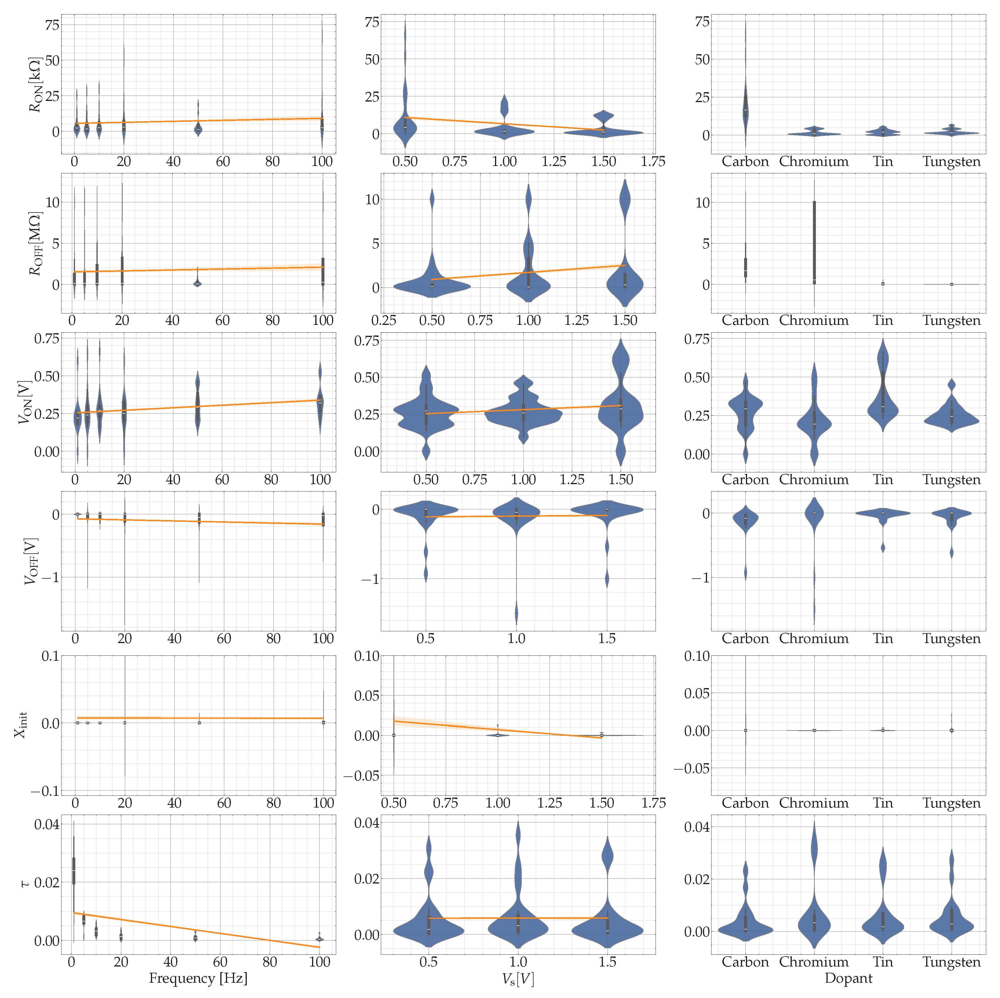
Figure 14.
A matrix of plots illustrating the variation in MMS model parameter values (y-axis) with linear trend lines, depending on the doping of memristors and excitation parameters (x-axis), is presented.
Figure 14.
A matrix of plots illustrating the variation in MMS model parameter values (y-axis) with linear trend lines, depending on the doping of memristors and excitation parameters (x-axis), is presented.
Table 1.
Box constraints on individual parameters during optimization for the MMS model.
Table 1.
Box constraints on individual parameters during optimization for the MMS model.
| Parameter |
Range |
Parameter |
Range |
|
|
|
|
|
|
|
|
|
|
|
|
Table 2.
Box constraints on individual parameters during optimization for the VTEAM model.
Table 2.
Box constraints on individual parameters during optimization for the VTEAM model.
| Parameter |
Range |
Parameter |
Range |
|
|
|
|
|
|
|
|
|
|
|
|
|
|
|
|
|
|
|
|
Table 3.
Box constraints on individual parameters during optimization for the Yakopcic model.
Table 3.
Box constraints on individual parameters during optimization for the Yakopcic model.
| Parameter |
Range |
Parameter |
Range |
|
|
|
|
|
|
|
|
|
|
|
|
|
|
|
|
|
|
|
|
| b |
|
|
|
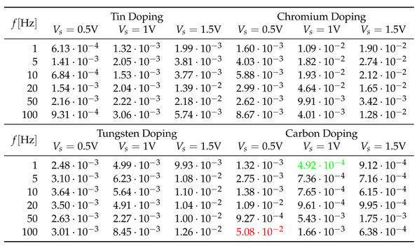
Table 4.
The objective function values for optimizing the MMS model when supplying the system with sinusoidal voltage of various parameters. The minimum value of the objective function is marked in green, while the maximum is marked in red.
Table 4.
The objective function values for optimizing the MMS model when supplying the system with sinusoidal voltage of various parameters. The minimum value of the objective function is marked in green, while the maximum is marked in red.
Table 5.
The example of the achieved parameters values for the MMS model for which the lowest objective function value was obtained(
). The memristor and excitation signal parameters can be found in the
Table 4.
Table 5.
The example of the achieved parameters values for the MMS model for which the lowest objective function value was obtained(
). The memristor and excitation signal parameters can be found in the
Table 4.
| Parameter |
Value |
Parameter |
Value |
|
|
|
|
|
|
|
|
|
|
|
|
Table 6.
The averaged objective function values for each type of memristor doping with after optimizing MMS model.
Table 6.
The averaged objective function values for each type of memristor doping with after optimizing MMS model.
| Doping |
Chromium |
Tin |
Tungsten |
Carbon |
|
|
|
|
|
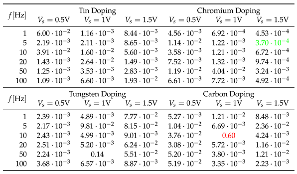
Table 7.
The objective function values for optimizing the VTEAM model when supplying the system with sinusoidal voltage of various parameters. The minimum value of the objective function is marked in green, while the maximum is marked in red.
Table 7.
The objective function values for optimizing the VTEAM model when supplying the system with sinusoidal voltage of various parameters. The minimum value of the objective function is marked in green, while the maximum is marked in red.
Table 8.
The achieved parameters values of the VTEAM model for which the lowest objective function value was obtained ().
Table 8.
The achieved parameters values of the VTEAM model for which the lowest objective function value was obtained ().
| Parameter |
Value |
Parameter |
Value |
|
|
|
|
|
|
|
|
|
|
|
|
|
6 |
|
2 |
|
|
|
|
Table 9.
The averaged objective function values for each type of memristor doping with after optimizing VTEAM model.
Table 9.
The averaged objective function values for each type of memristor doping with after optimizing VTEAM model.
| Doping |
Chromium |
Tin |
Tungsten |
Carbon |
|
|
|
|
|
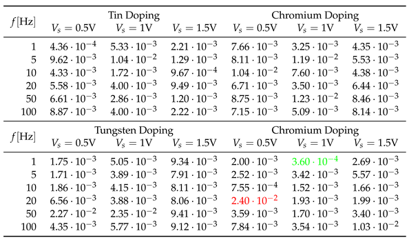
Table 10.
The objective function values for optimizing the Yakopcic model when supplying the system with sinusoidal voltage of various parameters. The minimum value of the objective function is marked in green, while the maximum is marked in red.
Table 10.
The objective function values for optimizing the Yakopcic model when supplying the system with sinusoidal voltage of various parameters. The minimum value of the objective function is marked in green, while the maximum is marked in red.
Table 11.
The parameters obtained for the Yakopcic model for the lowest objective function value ().
Table 11.
The parameters obtained for the Yakopcic model for the lowest objective function value ().
| Parameter |
Value |
Parameter |
Value |
|
|
|
|
|
|
|
|
|
|
|
|
|
|
|
|
|
|
|
|
| b |
|
|
|
Table 12.
The averaged objective function values for each type of memristor doping after optimizing Yakopcic model.
Table 12.
The averaged objective function values for each type of memristor doping after optimizing Yakopcic model.
| Doping |
Chromium |
Tin |
Tungsten |
Carbon |
|
|
|
|
|
Table 13.
Mean values of the objective function for each of the models. The highest objective function is marked in red, while the lowest is marked in green
Table 13.
Mean values of the objective function for each of the models. The highest objective function is marked in red, while the lowest is marked in green
Table 14.
Mean values of the objective function for each of the models. The highest objective function is indicated in red, and the lowest in green.
Table 14.
Mean values of the objective function for each of the models. The highest objective function is indicated in red, and the lowest in green.

