Preprint
Article

Study on Structure Damage Identification Methods

Altmetrics

Downloads

56

Views

16

Comments

0

A peer-reviewed article of this preprint also exists.

This version is not peer-reviewed

Submitted:

26 August 2024

Posted:

28 August 2024

You are already at the latest version

Alerts
Abstract
In order to solve the problem of structure damage location and degree identification, the weighted mean of vectors algorithm (INFO), a high-performance optimization one, was first introduced to identify structure damage. The genetic algorithm (GA) are improved to obtain a refined genetic algorithm (RGA). An objective function is constructed by combining the dynamic response transfer-ratio without modal analysis. INFO and RGA algorithms are used to optimize the objective function for damage identification. Though simulations, the INFO, RGA, GA algorithms were used to identify the damage on a simply supported beam and cantilevered plate with different levels of noise and different frequency spacing of pickup points. The simulations verify the effectiveness of the three damage identification methods, and the INFO algorithm has the highest damage identification accuracy, the RGA is second and the GA is the worst.
Keywords: 
Subject: Engineering  -   Mechanical Engineering

1. Introduction

As more and more large-scale space engineering structures are put into use, it has become a hot topic for engineers and scholars in various countries to establish a matching structural health monitoring system for all-around safety assurance, and one of the most important aspects is how to effectively identify the damage of space structures, including damage localization and quantitative analysis of the damage degree.
Damage identification based on the difference in the dynamic properties of the structure before and after damage has been a hotspot of concern in the engineering community. This type of strategy determines the location and extent of damage by evaluating the correlation of the dynamic parameters of the healthy and damaged structure, which is essentially an inverse problem, and the finite element model updating technique is often applied to solve this type of inverse problem.
Damage identification methods based on finite element model updating can transform the damage identification problem into a constrained optimization problem, which generally starts with the establishment of an objective function for evaluating the structural relevance of health and damage, and is subsequently solved using an optimization algorithm to find an optimal solution. However, traditional optimization algorithms, such as the most rapid descent method and the conjugate gradient method, are not only slow to converge but also prone to fall into local optimum. Therefore, developing or searching for more powerful optimization algorithms for damage identification is of great significance for the development of this field.
With the rapid development of intelligent optimization algorithms in recent times, more and more scientists have studied this in depth and used it to solve optimization problems in damage identification. Qian C Y et al [1] utilized an improved cuckoo algorithm combining frequency and vibration factors for damage identification of Benchmark frames with significant results. Vaez S R H et al [2] proposed a hybrid genetic and particle swarm algorithm for damage identification of damaged thin plate models and achieved good results. Wan Z H et al [3] proposed a two-stage damage identification method based on augmented whale algorithm to successfully identify multiple damages in simply supported beams with thin plates. Mohan S C et al [4] successfully localized and quantified the damage on beams and planar frames using damage detection technique based on frequency response function and particle swarm algorithm. Miguel L F F et al [5] proposed a hybrid stochastic/deterministic optimization algorithm for damage identification, which is more accurate and efficient in identifying damages when compared to genetic, harmonic and particle swarm algorithms. Ding Z H et al [6] proposed a damage identification method based on artificial bee colony algorithm with hybrid search strategy and modal data and successfully identified the damage on truss model and plate model. Pan C D et al [7] proposed a damage identification method based on hybrid adaptive firefly algorithm and verified the validity of the proposed method by two-story rigid frame structure and beam model. Chen Z P et al [8] embedded the Nelder-Mead algorithm into a particle swarm algorithm to obtain a hybrid particle swarm algorithm and used it for damage identification, and verified the effectiveness and superiority of the method through numerical simulation of simply supported beams as well as experiments on rectangular cross-section steel beams. Ding Z et al [9] proposed a damage identification method based on sparse regularization, Bayesian inference of improved objective function and improved Jaya algorithm, and verified the feasibility of the method through truss structure simulation and reinforced concrete bridge experiment. Guilherme F G et al [10] proposed an optimization algorithm based on sunflower motion and successfully identified the damage in composite laminates by this algorithm. Alkayem N F et al [11] proposed a damage identification method based on social swarm algorithm, modal strain energy, and modal vibrational curvature and verified the effectiveness of the method by numerical simulation. Huang M S et al [12] proposed a damage identification method based on modal frequency strain energy assurance criterion, modal flexibility and enhanced moth flame optimization algorithm and verified the effectiveness of the method by simply supported beams and triple shear frames experiments. Minh H L et al [13] proposed an augmented particle swarm algorithm for solving the damage identification problem and successfully applied the method to the damage identification of power transmission towers. Li X L et al [14] proposed a multi-component particle swarm algorithm with cooperative learning for damage identification, which fuses four particle swarm algorithm variants to build a pool of strategies, and the numerical simulation results show that the algorithm possesses higher accuracy for damage identification compared to a single variant and other algorithms. Zhang G C et al [15] proposed a new hybrid algorithm based on Jaya and differential evolutionary algorithm, and at the same time, established the objective function through the adjacent acceleration correlation function to identify the damage of cantilever beams and other models, and the results show that the method has high accuracy and computational efficiency. Li Y F et al [16] proposed a hybrid K-clustering mean optimization algorithm and used it for the identification of damage of small experimental dams, and the results show that this algorithm has high accuracy and computational efficiency for the identification of large and complex structures. The results show that the algorithm has high identification accuracy and computational efficiency, and has high potential for identifying the damage of large and complex structures. Thanh S T et al [17] proposed the goby joint search algorithm and used it for damage identification of Guangzhou Tower, the results show that this algorithm has higher damage identification accuracy compared to GAs, genetic particle swarm hybrid algorithms and so on. Muhammad I S et al [18] proposed a damage identification method based on hybrid YUKI-ANN algorithm with modal strain energy change ratio and successfully applied it for damage identification in plywood.
In this paper, the improved non-uniform mutation approach, improved mutation rate and crossover rate variation approach are added to the GA [19] to obtain the RGA and a high-performance optimization algorithm—INFO [20] is introduced. Next, an objective function based on the dynamic response transfer-ratio is established, which balances the sensitivity of each part of the function to damage by weighting factors calculated from the damage classification. Finally, taking simply supported beam and cantilever plate as objects, GA, RGA and INFO are utilized to identify a variety of damage cases under different levels of noises and different frequency spacing of pickup points, to verify the effectiveness of the methods and compare the damage identification effect of the algorithms.

2. Genetic Algorithm Refinement

The GA has strong global search performance, high efficiency and robustness, but subsequent studies have also shown that the GA performs poorly in local search ability, and the algorithm itself is prone to immature, slow convergence and degradation and other problems. To address these problems, this paper improves the mutation operator, crossover and mutation rate. The operations of the RGA are as follows (Figure 1 depicts the flow of the RGA).
(1) Selection and crossover
The selection operation in the paper adopts the roulette wheel approach, while adding the elite retention strategy. And the crossover operation adopts arithmetic crossover, which selects any two bodies in the parent generation for linear combination to produce a new individual, which can be expressed as
G A 1 g t + 1 = λ ⋅ G A 2 g t + 1 − λ ⋅ G A 1 g t G A 2 g t + 1 = λ ⋅ G A 1 g t + 1 − λ ⋅ G A 2 g t
Where G A 1 g t and G A 2 g t are the individuals of the g t th generation, G A 1 g t + 1 and G A 2 g t + 1 are the individuals of the g t +1th generation, and λ is a random number within the range 0 , 1 . To ensure that the crossover individuals do not exceed the specified range, a bounding judgment is added. Figure 2 displays the arithmetic crossover.
In this paper, the RGA uses a modified non-uniform mutation approach, randomly selecting individuals and generating a non-uniform perturbation to them that varies according to the number of evolutionary generations, to improve the algorithm's ability to search for the focal region, which can be expressed as
G n e w g t = G o l d g t + G o l d g t ⋅ λ 1 ⋅ 1 − g t M a x g 0.84 t b     λ 2 ≥ 0.5 G o l d g t − G o l d g t ⋅ λ 1 ⋅ 1 − g t M a x g 0.84 t b     λ 2 < 0.5
where G o l d g t and G n e w g t denote the unmutated and mutated individuals in the g t th generation respectively, M a x g are the maximum number of generations, λ 1 and λ 2 are random number within the range 0 , 1 . t b is a suitable perturbation parameter, which is taken as 3.7 in this paper. To ensure that the new individuals after mutation will not exceed the specified range, this step also requires boundary judgment.
(3) Mutation rate and crossover rate
In this paper, the RGA adopts a modified crossover rate and mutation rate change method, in which, on the one hand, the exponential function is used to increase the strength of crossover and mutation to increase the diversity of the population, so as not to let the population tend to a single dominant individual and fall into the local optimum, and on the other hand, the good individuals will be retained due to the small crossover rate and mutation rate, and the poor individuals will disappear rapidly due to the large mutation rate and crossover rate. The modified method can be expressed as follows
P I c = 0.84 f i t max − f i t avg f i t avg − f i t min + e p s 2       f i t max − f i t a v g f i t a v g − f i t min + e p s < 1 and p o p 1 ≥ p o p 2 p i c 1 − p i c 1 − p i c 2 f i t wb − f i t min f i t max − f i t min       otherwise
P I m = 0 . 12 f i t max − f i t avg f i t avg − f i t min + e p s 2       f i t max − f i t a v g f i t a v g − f i t min + e p s < 1 and p o p 1 ≥ p o p 2 p i m 1 − p i m 1 − p i m 2 f i t w 1 − f i t min f i t max − f i t min       otherwise
Where P I c and P I m represent the crossover rate and mutation rate respectively, p i c 1 and p i c 2 are the crossover calculation coefficients with values of 0.9 and 0.6 respectively, p i m 1 and p i m 2 are the variation calculation coefficients with values of 0.1 and 0.01 respectively, f i t max and f i t min denote the maximum and minimum fitness values of individuals in population respectively, f i t avg denotes the mean value of population fitness, f i t wb denotes the larger fitness value of the two individuals that are about to cross, and f i t w 1 denotes the fitness value of the individual that is about to take part in the mutation, p o p 1 and p o p 2 denote the number of individuals in the population with higher and lower fitness values than the population mean respectively, and e p s is an infinitesimal positive integer.

3. Weighted Mean of Vectors Algorithm

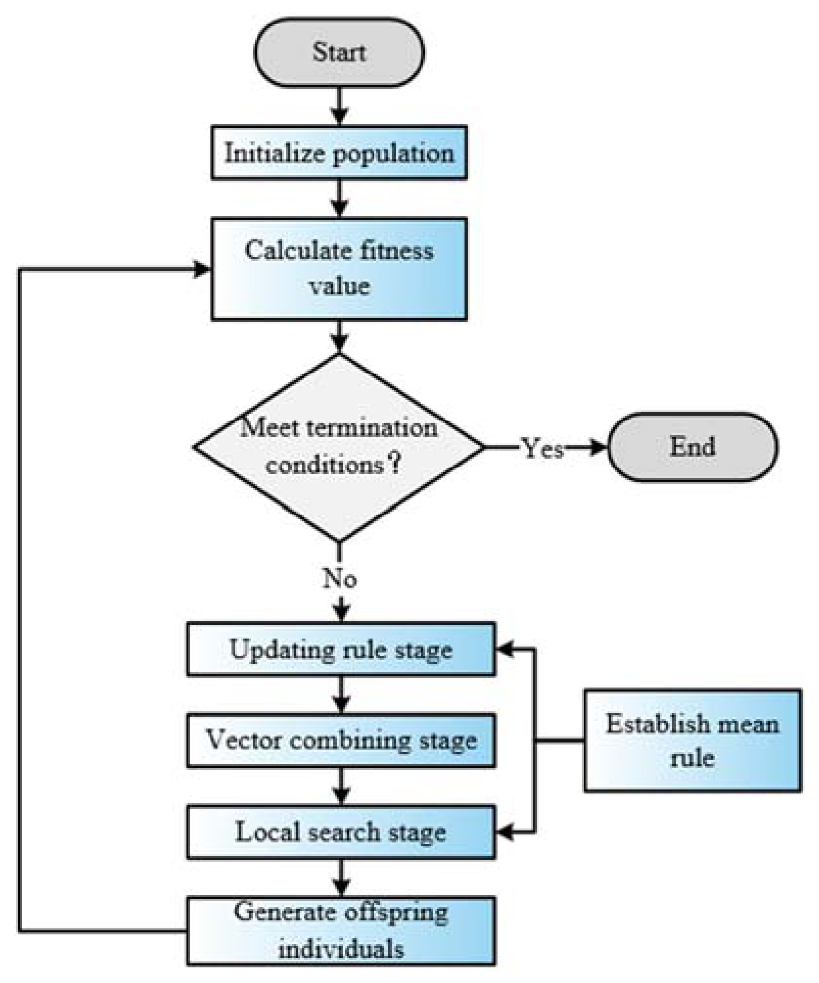
INFO is a new type of intelligent algorithm proposed by Dr. Ahmadianfar et al. in 2022. The algorithm applies the improved weighted mean idea to the entity structure, and updates the solution vector through three core steps: updating rules, vector combination and local search. It has the advantages of strong optimization ability and fast convergence speed. The specific implementation process is described as follows (Figure 3 depicts the flow of the INFO).
(1) Updating rule stage
INFO's updating rule operator uses the weighted mean of the vectors to create new vectors and performs an efficient global search in this way. Firstly, INFO has to randomly select three difference vectors from all solution vectors of each generation to calculate the vector-weighted mean value W M 1 i t , and at the same time select the best, better and worst solution vectors of the total solution vectors to calculate the vector-weighted mean value W M 2 i t , which can be expressed respectively as
W M 1 i t = s c ⋅ r h 1 ⋅ u g x i t − u g y i t + r h 2 ⋅ u g x i t − u g z i t + r h 3 ⋅ u g y i t − u g z i t r h 1 + r h 2 + r h 3 + e p + e p ⋅ r a n d 1 ⋅ o e
W M 2 i t = s c ⋅ r h 4 ⋅ u b s i t − u b t i t + r h 5 ⋅ u b s i t − u w s i t + r h 6 ⋅ u b t i t − u w s i t r h 4 + r h 5 + r h 6 + e p + e p ⋅ r a n d 2 ⋅ o e
where r h 1 = cos o b j u g x i t − o b j u g y i t + π ⋅ exp − o b j u g x i t − o b j u g y i t max o b j u g x i t , o b j u g y i t , o b j u g z i t ,
r h 2 = cos o b j u g x i t − o b j u g z i t + π ⋅ exp − o b j u g x i t − o b j u g z i t max o b j u g x i t , o b j u g y i t , o b j u g z i t
r h 3 = cos o b j u g y i t − o b j u g z i t + π ⋅ exp − o b j u g y i t − o b j u g z i t max o b j u g x i t , o b j u g y i t , o b j u g z i t
r h 4 = cos o b j u b s i t − o b j u b t i t + π ⋅ exp − o b j u b s i t − o b j u b t i t o b j u w s i t
r h 5 = cos o b j u b s i t − o b j u w s i t + π ⋅ exp − o b j u b s i t − o b j u w s i t o b j u w s i t
r h 6 = cos o b j u b t i t − o b j u w s i t + π ⋅ exp − o b j u b t i t − o b j u w s i t o b j u w s i t Where o b j u is the value of the objective function, u g x i t , u g y i t , and u g z i t are individuals in the i t th generation. g x , g y , and g z are different integers randomly chosen from the range 0 , 1 , N P is the population size, e p is an infinitesimal constant, r a n d 1 and r a n d 2 are random numbers within the range 0 , 1 , o e is a vector whose all elements are 1, u b s i t , u b t i t and u w s i t are the best, better, and worst individuals in the i t th generation respectively, s c is a scaling factor, which can be expressed as follows
s c = 4 r a n d 3 − 2 ⋅ exp − 4 i t M a x i t
Where r a n d 3 is a random number within the range 0 , 1 , M a x i t is the maximum number of evolutionary generations.
Next, INFO uses the W M 1 i t and W M 2 i t constructs the MeanRule , which can be expressed as follows
MeanRule = θ ⋅ W M 1 i t + 1 − θ ⋅ W M 2 i t
Where θ is a random number within the range 0 , 0.5 . Finally, to further improve the global search capability of the algorithm, an additional convergence acceleration module is added, which makes full use of the optimal solution vectors in each generation to change the current solution vectors in the search space. Therefore, the final update rule formula for INFO is expressed as follows
cz 1 n u i t = u n u i t + σ ⋅ MeanRule + r a n d n 1 ⋅ u b s i t − u g x i t o b j u b s i t − o b j u g x i t + 1 r a n d 4 < 0.5 u g x i t + σ ⋅ MeanRule + r a n d n 2 ⋅ u g y i t − u g z i t o b j u g y i t − o b j u g z i t + 1 r a n d 4 ≥ 0.5
cz 2 n u i t = u b s i t + σ ⋅ MeanRule + r a n d n 3 ⋅ u g x i t − u g y i t o b j u g x i t − o b j u g y i t + 1 r a n d 4 < 0.5 u b t i t + σ ⋅ MeanRule + r a n d n 4 ⋅ u g x i t − u g y i t o b j u g x i t − o b j u g y i t + 1 r a n d 4 ≥ 0.5
where cz 1 n u i t and cz 2 n u i t are the new solution vectors of the i t th generation, n u = 1 , 2 ,…, N P ,and n u ≠ g x ≠ g y ≠ g z , r a n d 4 is a random number within the range 0 , 1 , r a n d n 1 , r a n d n 2 , r a n d n 3 and r a n d n 4 are standard normally distributed random numbers. σ is the scaling factor, which can be expressed as follows
σ = 4 r a n d 5 − 2 ⋅ exp − 4 i t M a x i t
where r a n d 5 is a random number within the range 0 , 1 .
(2) Vector combining stage
To improve the local search capability of INFO, the solution vectors cz 1 n u i t and cz 2 n u i t computed in the updating rule stage are combined to generate a new solution vector c v n u i t , which can be expressed as follows
c v n u i t = c z 1 n u i t + n s â‹… c z 1 n u i t − c z 2 n u i t       r a n d 6 < 0.5   and   r a n d 7 < 0.5 c z 2 n u i t + n s â‹… c z 1 n u i t − c z 2 n u i t       r a n d 6 < 0.5   and   r a n d 7 ≥ 0.5 u n u i t           r a n d 6 ≥ 0.5
where n s = 0.05 r a n d n 5 , r a n d n 5 is a standard normally distributed random number, r a n d 6 and r a n d 7 are random numbers within the range 0 , 1 .
(3) Local search stage
The local search stage will create a new solution vector c v s i t based on the mean rule to further enhance the local search capability of INFO, and the specific implementation formula can be expressed as
c v s i t = u b s i t + r a n d n 6 â‹… MeanRule + r a n d n 7 â‹… u b s i t − u g x i t         r a n d 8 < 0.5   and r a n d 9 < 0.5 u r n d i t + r a n d n 8 â‹… MeanRule + r a n d n 9 â‹… v s 1 â‹… u b s i t − v s 2 â‹… u r n d i t   r a n d 8 < 0.5   and r a n d 9 ≥ 0.5
Where u rnd i t = ϕ ⋅ u g x i t + u g y i t + u g z i t 3 + 1 − ϕ ⋅ ϕ ⋅ u b t i t + 1 − ϕ ⋅ u b s i t
v s 1 = 2 r a n d 10       η > 0.5 1       η ≤ 0.5 , v s 2 = r a n d 11       η < 0.5 1       η ≥ 0.5
where ϕ , r a n d 8 , r a n d 9 , η , r a n d 10 and r a n d 11 are random numbers within the range 0 , 1 , r a n d n 6 , r a n d n 7 , r a n d n 8 and r a n d n 9 are standard normally distributed random numbers.

4. Objective Function

The use of intelligent algorithms to localize and quantify structural damage requires the establishment of a corresponding objective function. Dynamic response transfer-ratio is combined with modal assurance criterion [21] to define the following assurance criterion function of transfer-ratio T F A C ω ,dynamic response transfer-ratio is combined with amplitude correlation coefficient [22] to define the following amplitude correlation function of transfer-ratio T F A L ω , which can be expressed as
T F A C ω = T F Τ ω T F ω , α 2 T F Τ ω T F ω T F Τ ω , α T F ω , α
T F A L ω = 2 ⋅ T F Τ ω T F ω , α T F Τ ω T F ω + T F Τ ω , α T F ω , α
where T F ω is the dynamic response transfer-ratio vector measured, and T F ω , α is the dynamic response transfer-ratio vector calculated based on the finite element numerical modeling theory. The objective function is established based on T F A C ω and T F A L ω , which can be expressed as
o b j 1 = η 1 ⋅ B J 1 + η 2 ⋅ B J 2
where
B J 1 = ∑ z = 1 n u m 1 − T F A C ω z   B J 2 = ∑ z = 1 n u m 1 − T F A L ω z
where n u m is the number of selected frequency point, T F A C ω z is the assurance criterion function value of transfer-ratio at the given frequency ω z , and T F A L ω z is the amplitude correlation function value of transfer ratio at the given frequency ω z . η 1 and η 2 are the different weighting factors.

5. Weighting Factors and Mean Error

Since the assurance criterion function and the amplitude correlation function of the dynamic response transfer-ratio have different sensitivities to damage, it is likely that damage will lead to large differences in the values of B J 1 and B J 2 . This can easily lead to intelligent algorithms taking one part of the objective function as the dominant part of the constrained optimization problem when solving the problem, which in turn makes the role of the other part of the objective function significantly weakened.
In this paper, according to the method of literature [23], the weighting factors are calculated and substituted into the objective function, so as to weaken the numerical difference between B J 1 and B J 2 to make the intelligent algorithm solution more accurate. The specific calculation method is expressed as follows
η 1 = ∑ n a = 1 n x ∑ n b = 1 n y B J 2 n a , n b / B J 1 n a , n b ∑ n a = 1 n x ∑ n b = 1 n y B J 2 n a , n b / B J 1 n a , n b + n x 2
η 2 = 1 − η 1
Where n x is the number of units in the structure division, n y is the number of damage grading, B J 1 n a , n b and B J 2 n a , n b are the values of B J 1 and B J 2 for the n a th unit at damage level n b respectively. A total of ten levels of damage grading were chosen for this paper, with unit damage levels of 0.1, 0.2, 0.3, 0.4, 0.5, 0.6, 0.7, 0.8, 0.9 and 0.99 in descending order.
In order to evaluate the accuracy of the intelligent algorithm in identifying the damage degree of the preconfigured damage units (the target damage units in this paper refer to the preconfigured damage units in the damage cases) in each damage case in the simulation, the mean error E m will be introduced, which is denoted as
E m = 1 n e ∑ φ = 1 n e α φ t h − α φ r e α φ t h × 100 %
Where α φ t h and α φ r e denote the preconfigured damage degree of the φ th preconfigured damage unit and the damage degree identified by the algorithm under a certain case respectively, and n e denotes the number of preconfigured damage units in the case.

6. Numerical Simulation

In order to verify the identification accuracy of the damage identification method based on the RGA and INFO under different levels of noise and different frequency point spacing, a numerical case study was carried out in MATLAB for simply supported beams and cantilever plates (the damage identification results in this paper are the average values obtained after ten runs). In addition, the mutation rate and crossover rate of the standard GA as a comparison are set to 0.2 and 0.4 respectively, and the number of populations and iterations of the three algorithms are set to 120 and 800 respectively. The acceleration response signal added white noise into can be expressed as follows
A c c 1 = A c c 0 â‹… 1 + n o i â‹… r d n
where A c c 0 and A c c 1 are the acceleration response signals before and after the noise interference, n o i is the noise level, and r d n is a standard normally distributed random number.

6.1. Simulation of simply supported beam

The model of the simply supported beam is shown in Figure 4, which is divided into 12 units, the axial length of the beam is 1.2 m, and the cross-section is a rectangle with a width of 0.05 m and a height of 0.015 m. The modulus of elasticity of the material is set to 2.06 × 10¹¹ Pa, Poisson's ratio is 0.3, and the density is 7850 kg/m3. The first five orders of nature frequencies of the model are 24.19 Hz, 96.66 Hz, 217.07 Hz, 384.76 Hz, and 598.42 Hz.
In the simulation, the single-point excitation is applied to node 3 of the model, and the Y-direction transfer ratio of each node substituted into the objective function is calculated with the Y-direction acceleration response of node 2 as a reference. The frequency range of the objective function o b j 1 is taken from 1 Hz to 400 Hz ( including the first four orders of the nature frequencies of the model ), and 400 frequency points are taken at equal intervals of 1 Hz in the frequency range.
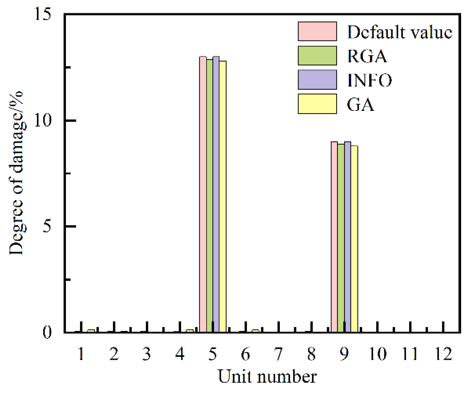
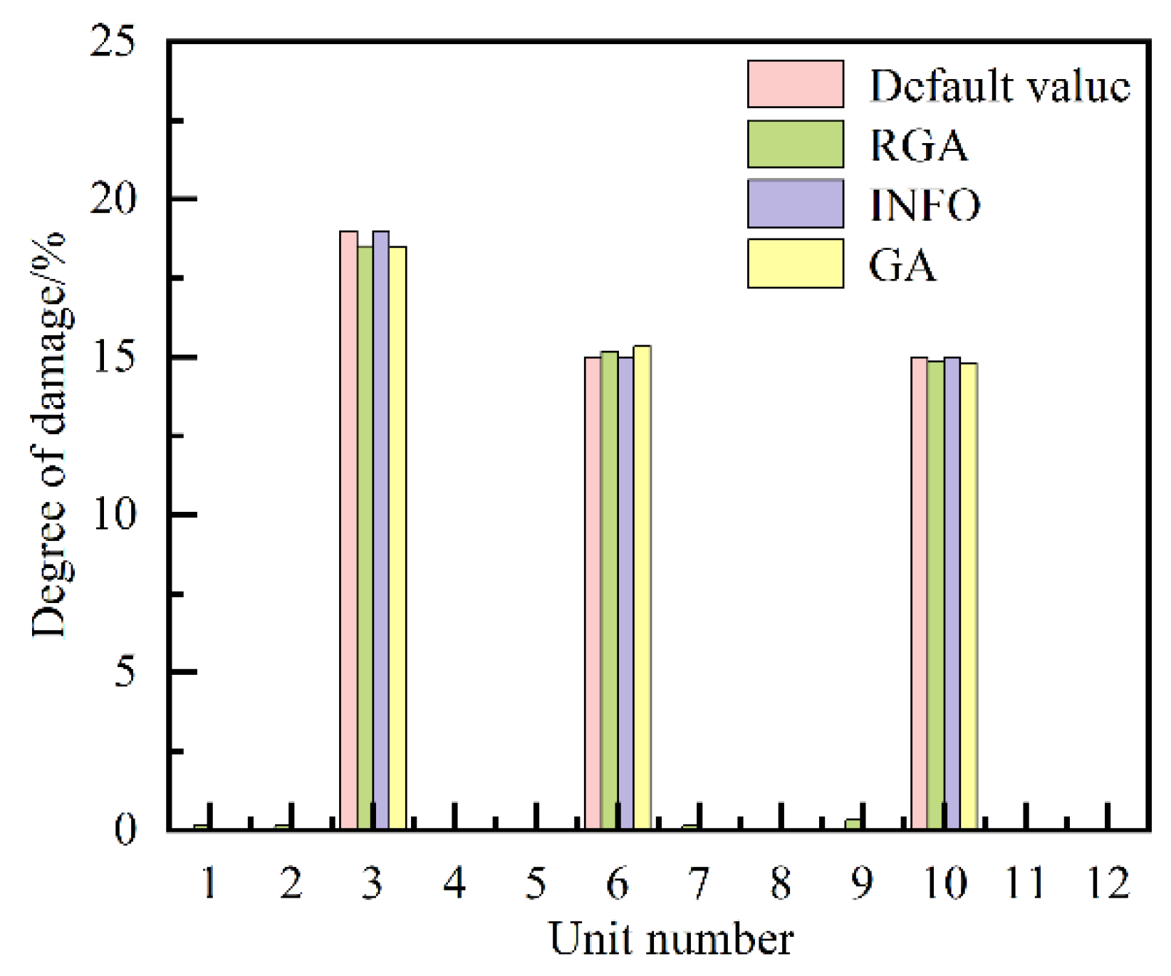
The three intelligent algorithms are used to identify the damage of the two damage cases of the simply supported beam in Table 1 in the absence of noise, and the results of the damage identification of each beam unit in Case 1 and Case 2 are shown in Figure 5 and Figure 6 , and the results of the identification of the target damage unit are shown in Table 2.
It can be observed from Figure 5 and Figure 6, the three algorithms can accurately locate the damages in Case 1 and in Case 2 without noise interference, and none of the three algorithms have obvious misjudgment units.
Further analysis of Table 2 shows that the mean errors of the target damage units identified by GA and RGA in Case 1 are 1.94% and 1.09% , in Case 2 are 2.02% and 1.60% respectively, while INFO has the highest identification accuracy without obvious errors for the two Cases.
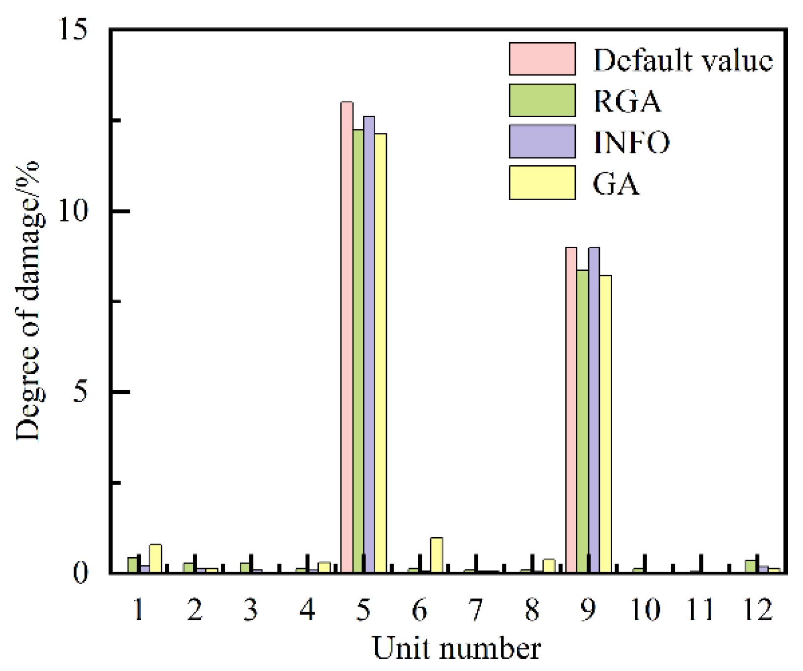
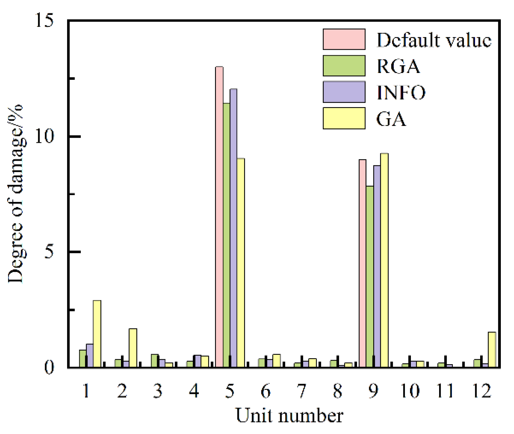
However, the measured response data will inevitably be affected by different levels of noise in practical engineering applications. When 1% and 3% noise were added to the Case 1, the damage identification results of each beam unit under the influence of two different levels of noise are shown in Figure 7 and Figure 8 respectively.
From Figure 7 and Figure 8, it can be found that all the three algorithms accurately identify the damage locations under the influence of 1% as well as 3% noise, but under the influence of 3% noise, there is a significant misjudgment for the GA for the damage identification of the simply-supported-beam model at the unit 1, 2 and 12.
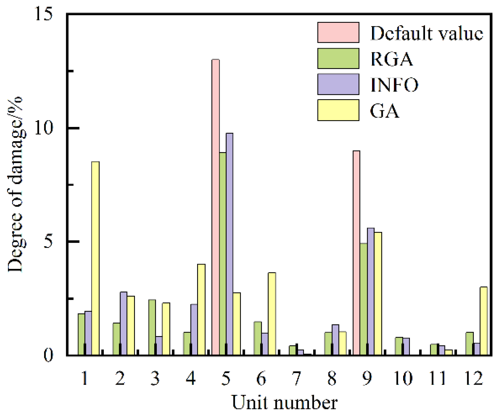
Figure 9 shows the damage identification results for each unit under 10% noise added to the Case 1.
From Figure 9, it can be found that under the influence of 10% noise, the three algorithms' damage identification results are significantly worse compared to ones of 1% and 3% noise, and there are many obvious misjudgment units, of which GA is relatively more affected by this level of noise, while the other two algorithms' damage identification results are better than that of GA.
The identification results under the influence of 1%, 3%, and 10% noise are shown in Table 3.
Table 3 (Case 1) shows that under the influence of 1%, 3% and 10% noise, the mean errors of the target damage units identified by GA are 7.74%, 16.68% and 59.31% , by RGA are 6.52%, 12.39% and 38.40%, and by INFO are 1.67%, 5.18% and 31.29%, respectively. It can be seen that INFO has the highest accuracy, RGA has the second and GA has the lowest accuracy in identifying the damage degree of the target unit. The mean error of the three algorithms in identifying the damage of the target unit in Case 1 increases significantly compared results of 10% noise with that of 1% and 3% noise, which is mainly due to the fact that too high a level of noise seriously affects the transfer ratio obtained and ultimately results in the failure to obtain a more accurate damage degree of the target unit, even if the value of the objective function is converged to a more close to the global optimum.
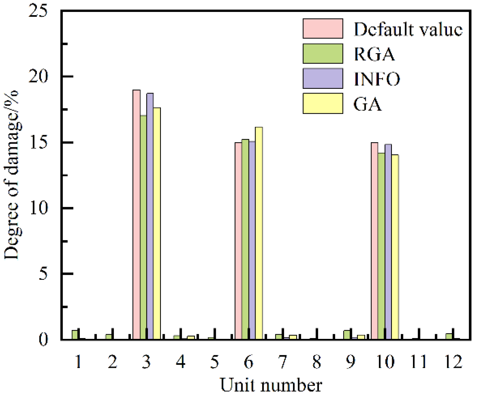
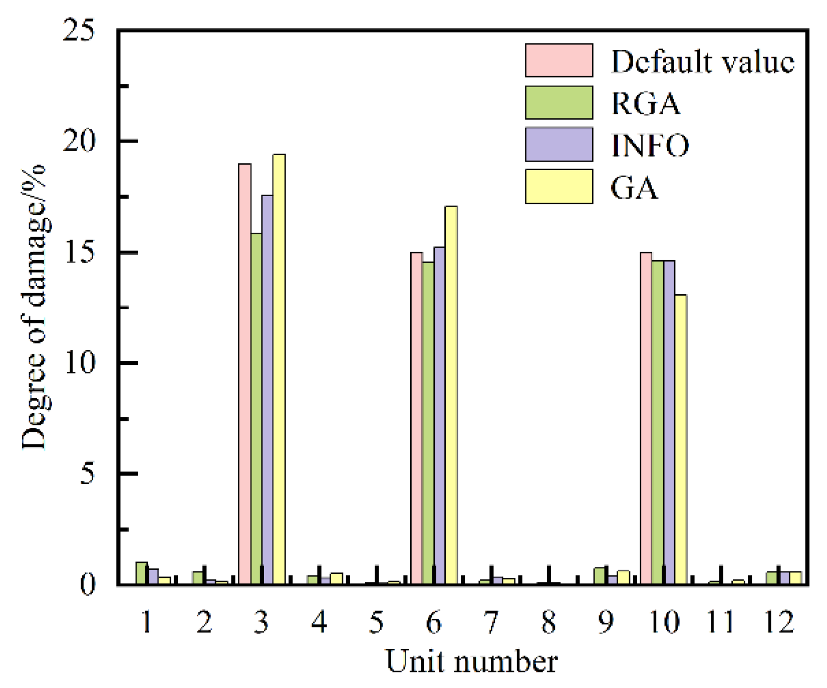
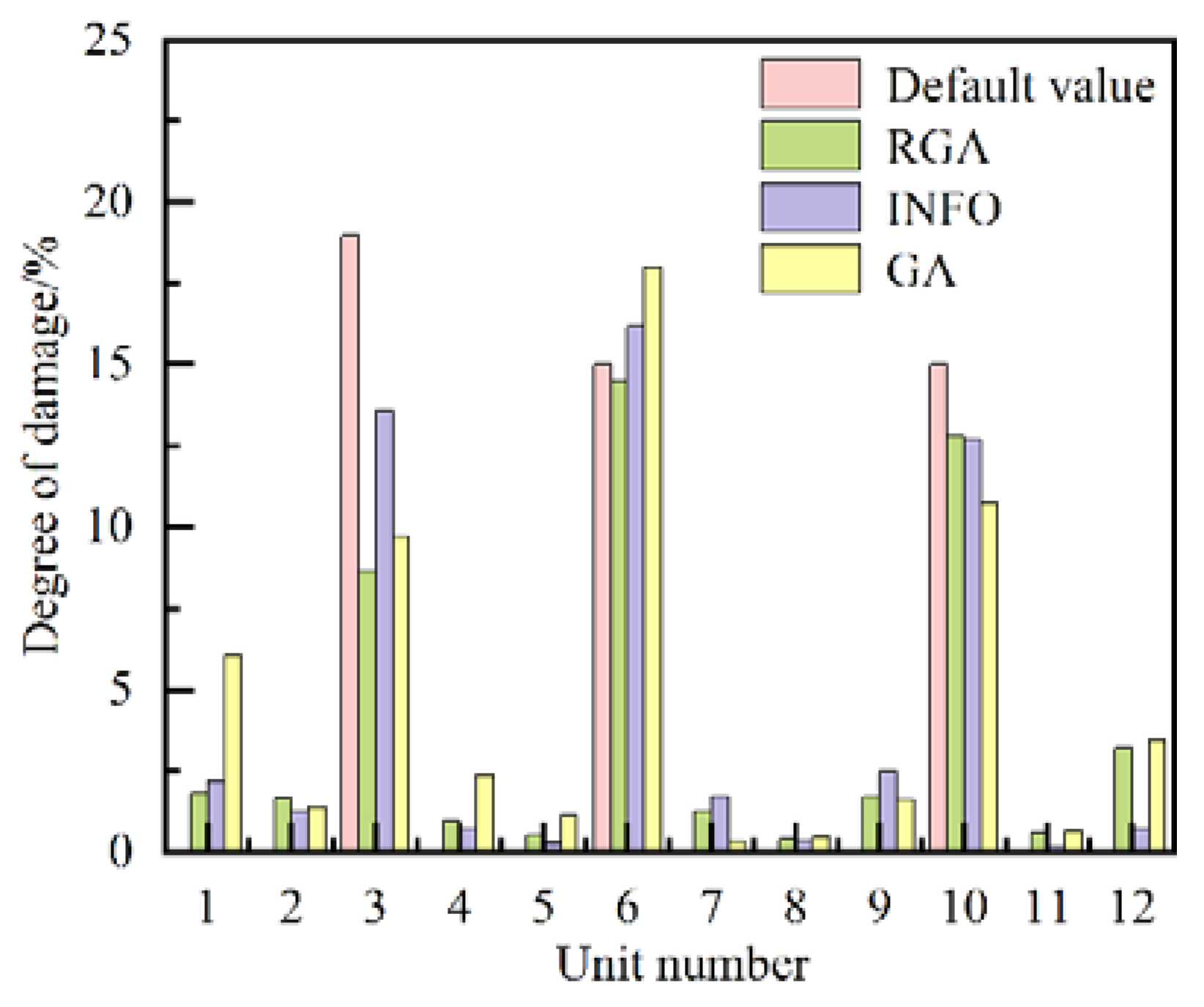
Subsequently, the same noise in Case 1 are added to the Case 2, and the results of damage identification of each unit under the influence of three different levels of noise are shown in Figure 10, Figure 11 and Figure 12 respectively.
From Figure 10, Figure 11 and Figure 12, it can be found that there is a same pattern as Case 1. But under the influence of 3% noise, not being same as Case 1, the damage identification using GA does not appear obvious misjudgment units, mainly due to the damage degree of the damage unit in Case 2 is larger and the identification results is not easy to be affected by the noise.
The results of identifying the target damage units (Case 2) under the influence of 1%, 3%, and 10% noise are shown in Table 4.
Table 4 (Case 2) shows that under the influence of 1%, 3% and 10% noise, the mean errors of the target damage units identified by GA are 7.10%, 9.67%, and 32.43%, by RGA are 5.75%, 7.31% and 24.09% and by INFO are 1.00%, 3.82% and 17.24%, respectively. Comparing the mean errors, it can be seen that INFO has the highest accuracy in identifying the damage degree of the target unit, RGA has the second highest accuracy and GA has the lowest accuracy.
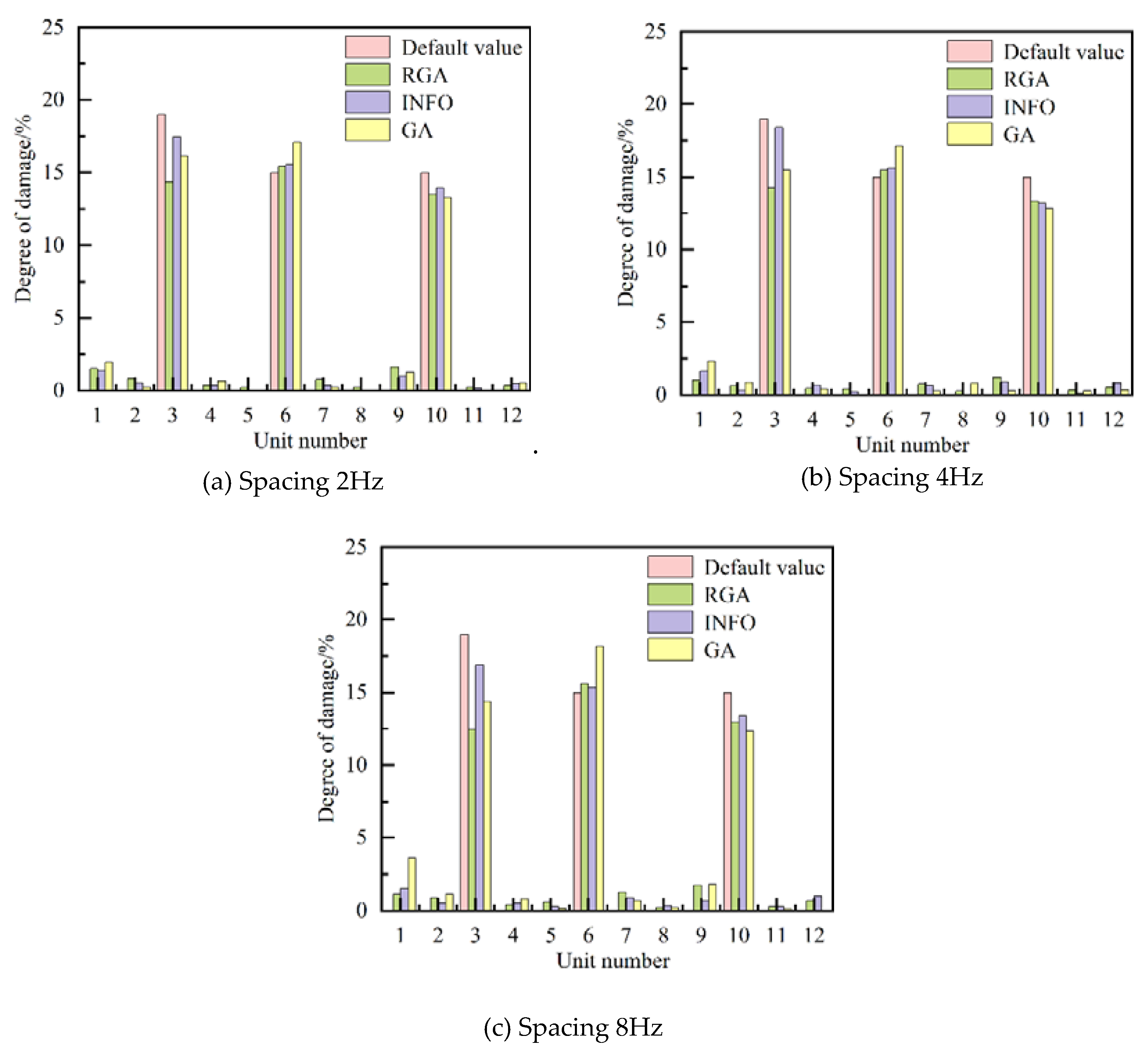
In the aforementioned simulation, more frequency points in a larger frequency range were used , leading to increased computation. so it is considered to reduce the frequency points. Keeping the frequency range from 1 Hz to 400 Hz unchanged , the following three scenarios were simulated for the Case 2: (1) take points at equal intervals of 2Hz for a total of 200 frequency points. (2) take points at equal intervals of 4Hz for a total of 100 frequency points. (3) and take points at equal intervals of 8Hz for a total of 50 frequency points. The damage identification results adding 3% noise are shown in Figure 13 and Table 5.
From Figure 13, it can be observed that under the influence of the same noise, the damage identification results of each beam unit at 2Hz spacing for the three algorithms are slightly worse than the aforementioned ones in the Figure 11 at 1Hz spacing, but there is no obvious difference in the identification results compared with 4Hz and 8Hz spacing.
Table 5 shows that, under the influence of the same noise, the mean errors of the target damage identified by the three methods at 2Hz spacing are 13.44%, 12.35%, and 6.26%, at 4Hz are 15.79%, 13.13%, and 6.47% and at 8Hz are 21.11%, 17.36%, and 8.06%, respectively. The identification accuracy for the three algorithms is getting lower and lower with the gradual increase of taking point spacing within the same frequency range, and the identification accuracy of INFO is the highest with the second highest identification accuracy for the RGA and the lowest identification accuracy of the GA.

6.2. Simulation of Cantilever Plate

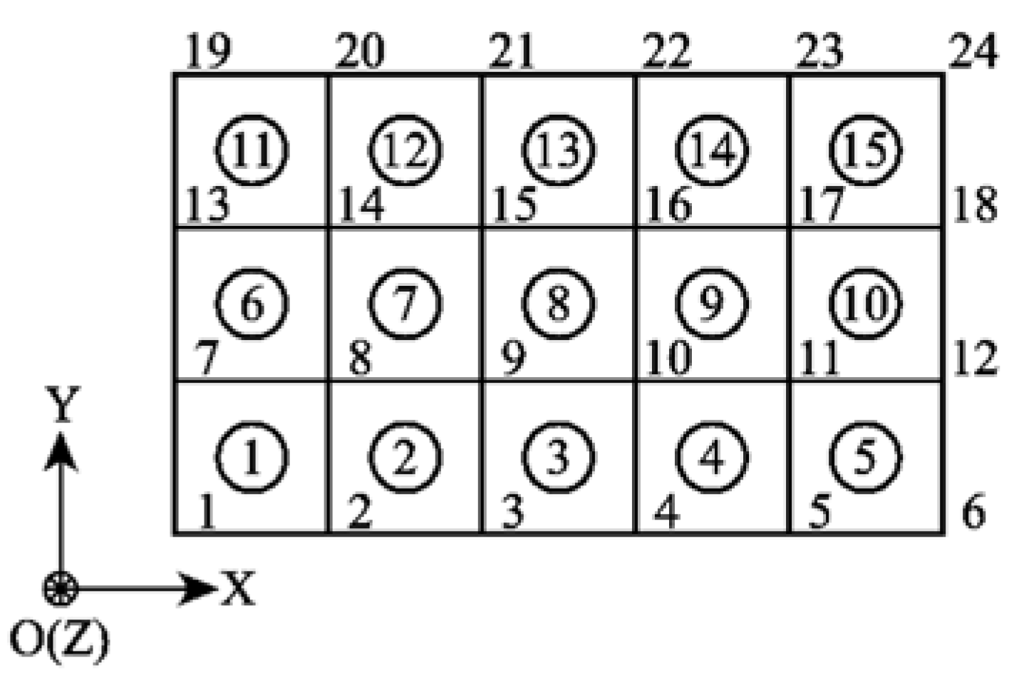
The cantilever plate model is shown in Figure 14, The length, width and thickness of the cantilever plate are 0.5 m, 0.3 m and 0.004 m respectively, the density of the structural material is 7850kg/m3, the modulus of elasticity is 2.06 × 10¹¹Pa, poisson ratio is 0.3, and it is divided into 15 plate-shell units, the length and width of each unit is 0.1m, and the left edge of the plate is fixed. The first five orders of its nature frequencies are 13.61 Hz, 50.21 Hz, 85.46 Hz, 167.02 Hz, and 236.78 Hz. The numbers above the nodes of the units are the nodes numbers, and the numbers inside the circles are the cell units numbers.
The cantilever plate numerical model is set up with two damage cases as shown in Table 6.
In the simulation, a single-point excitation is applied to node 18 of the cantilever plate model, and the Z-direction transfer ratio of each node substituted into the objective function is calculated with the Z-direction acceleration response of node 20 as a reference. The frequency range of the objective function o b j 1 is taken from 11Hz to 240Hz (including the first five orders of the nature frequency of the model), and 230 frequency points are taken at equal intervals of 1Hz.
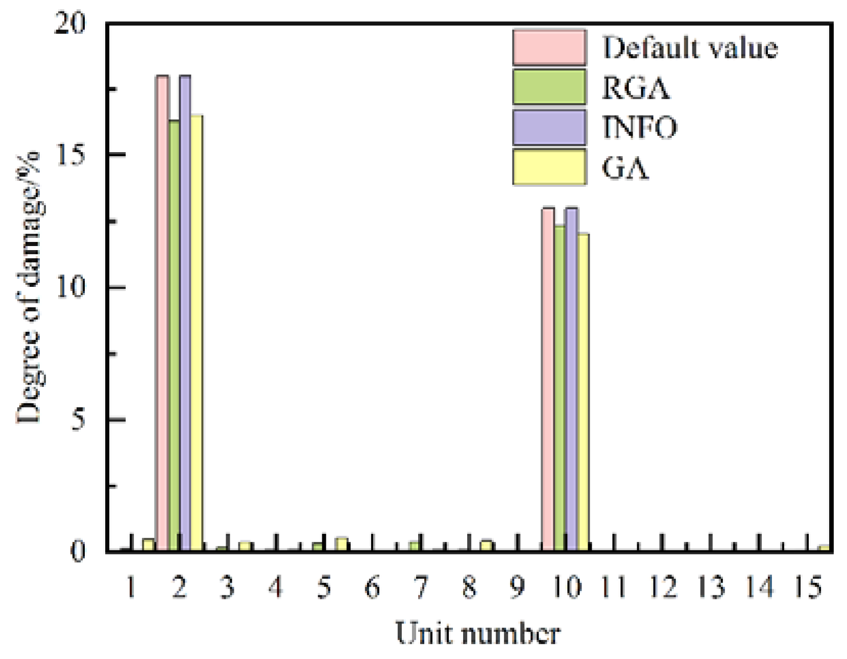
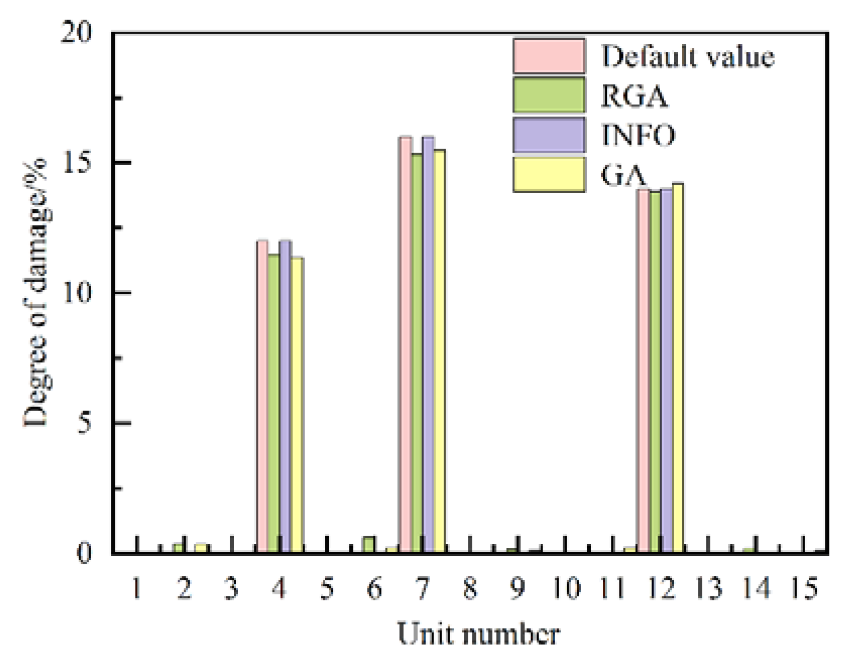
The three intelligent algorithms are used to identify the damage of the two damage cases of cantilever plate in Table 6 without adding noise. The results of the damage identification in Case 3 and Case 4 are shown in Figure 15, Figure 16, and Table 7.
It can be observed from Figure 15 and Figure 16 that the three intelligent algorithms can accurately localize the two damages in Case 3 and the three damages in Case 4 without any obvious misjudgment unit without noise interference.
Table 7 shows that the mean errors of the target damage units identified by GA and RGA in Case 3 are 7.82% and 7.38%, and in Case 4, are 3.36% and 3.11%, respectively, whereas there are significant identification errors in both cases for INFO.
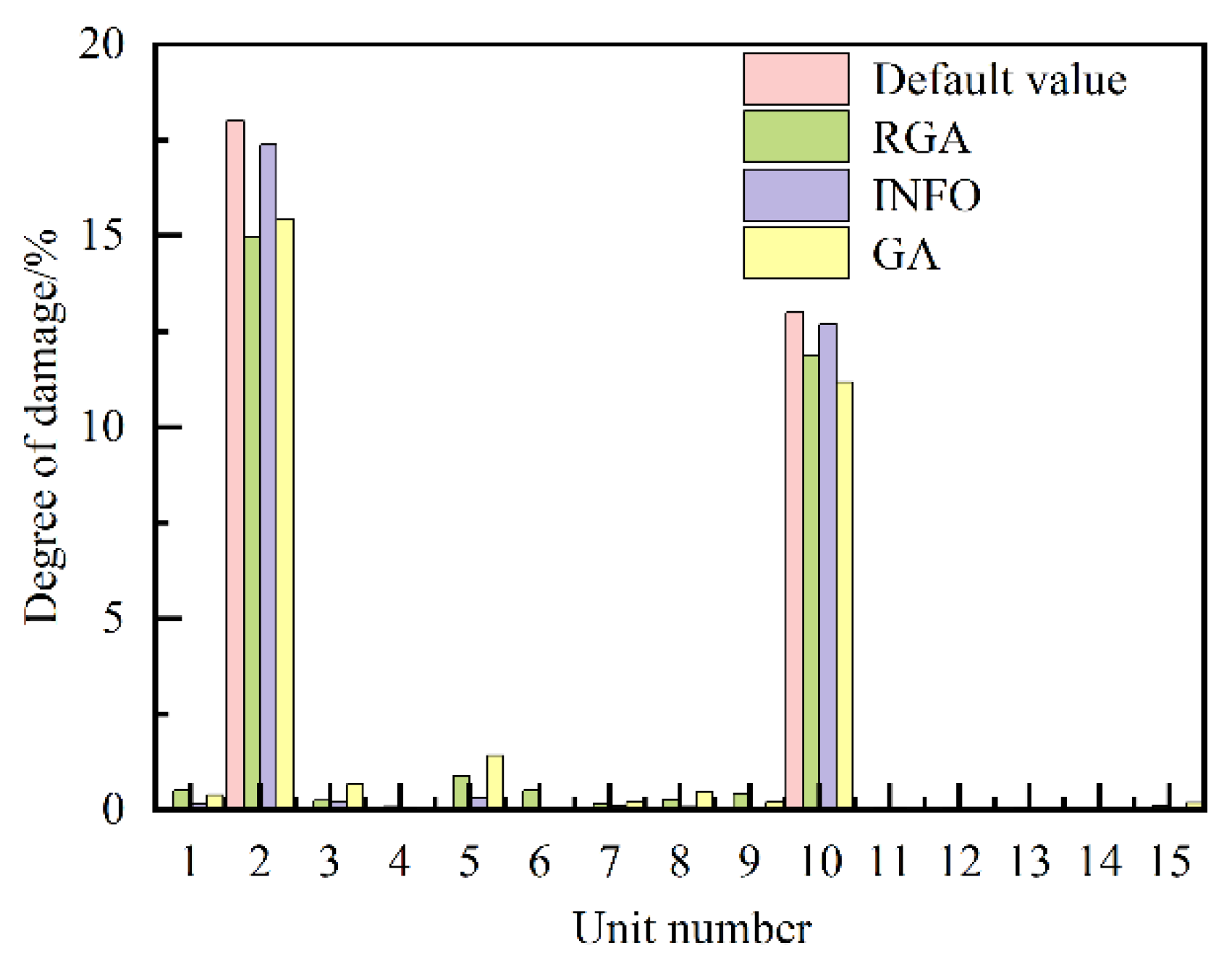
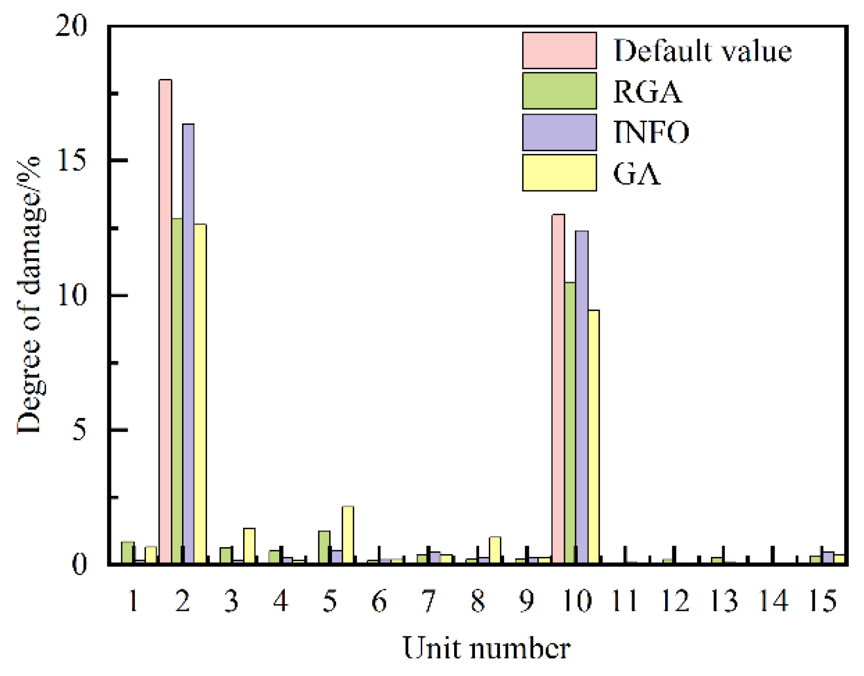
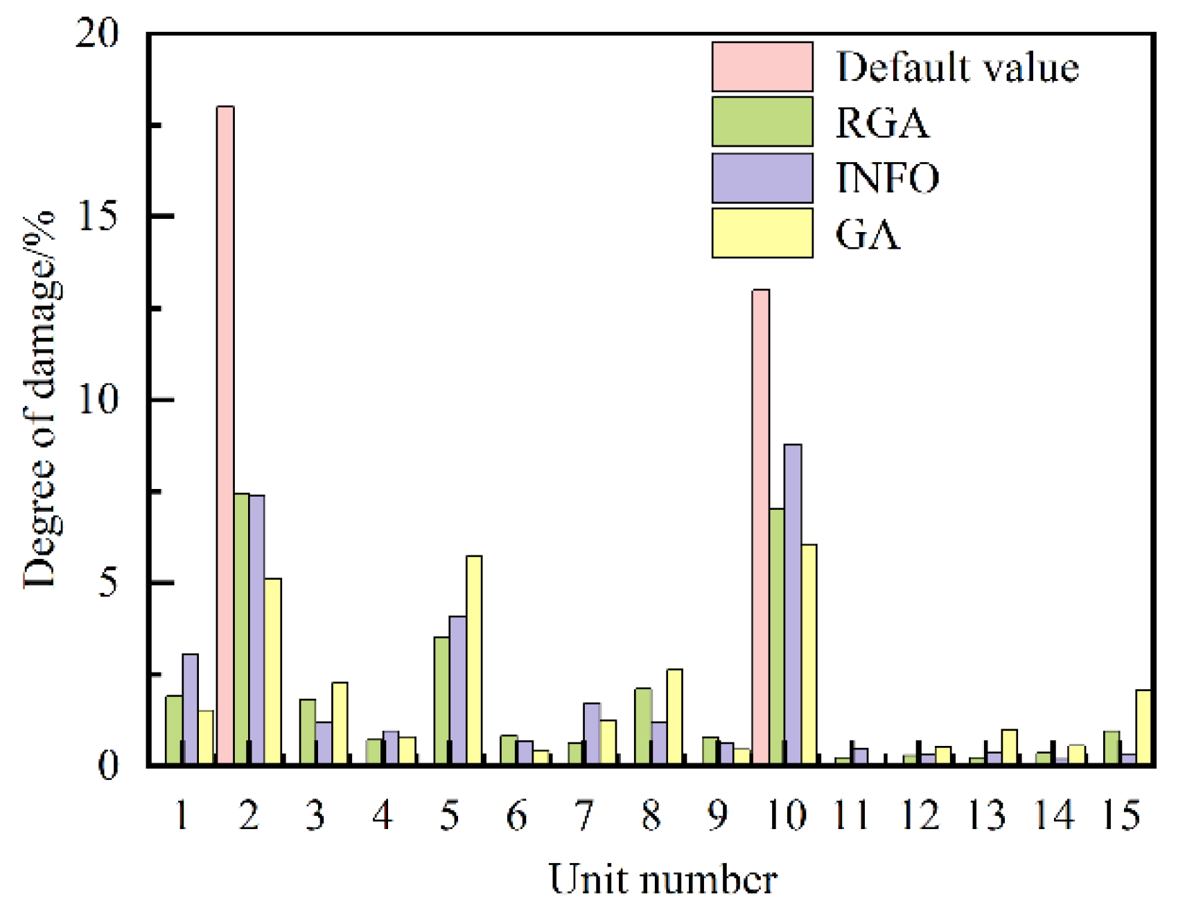
When 1%, 3% and 10% noise added to the cantilever plate damage Case 3. The results of damage identification under the influence of three different levels of noise are shown in Figure 17, Figure 18 , Figure 20 and Table 8, respectively.
From Figure 17, Figure 18 and Figure 19, it can be found that under the influence of 1% and 3% noise, GA, RGA and INFO can accurately locate the damage position of the cantilever plate, of which INFO has the best damage identification results without significant misjudgment units, while more significant misjudgment units are found for both GA and RGA and under the influence of 10% noise, there are many obvious misjudgment units for the three methods.
Table 8 (Case 3) shows that under the influence of 1%, 3% and 10% noise, the mean errors of the target damage units identified by GA are 14.18%, 28.64% and 62.47% , by RGA are 12.77%, 24.02% and 52.34%, and by INFO are 2.90%, 6.80% and 45.65%, respectively. It can be seen that INFO has the highest accuracy, RGA has the second highest accuracy and GA has the lowest accuracy.
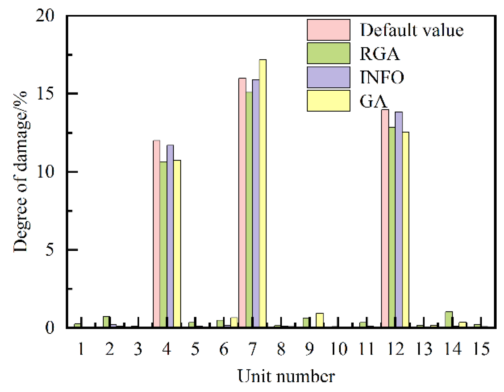
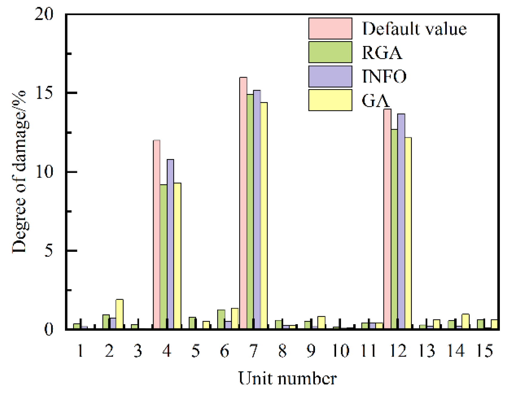
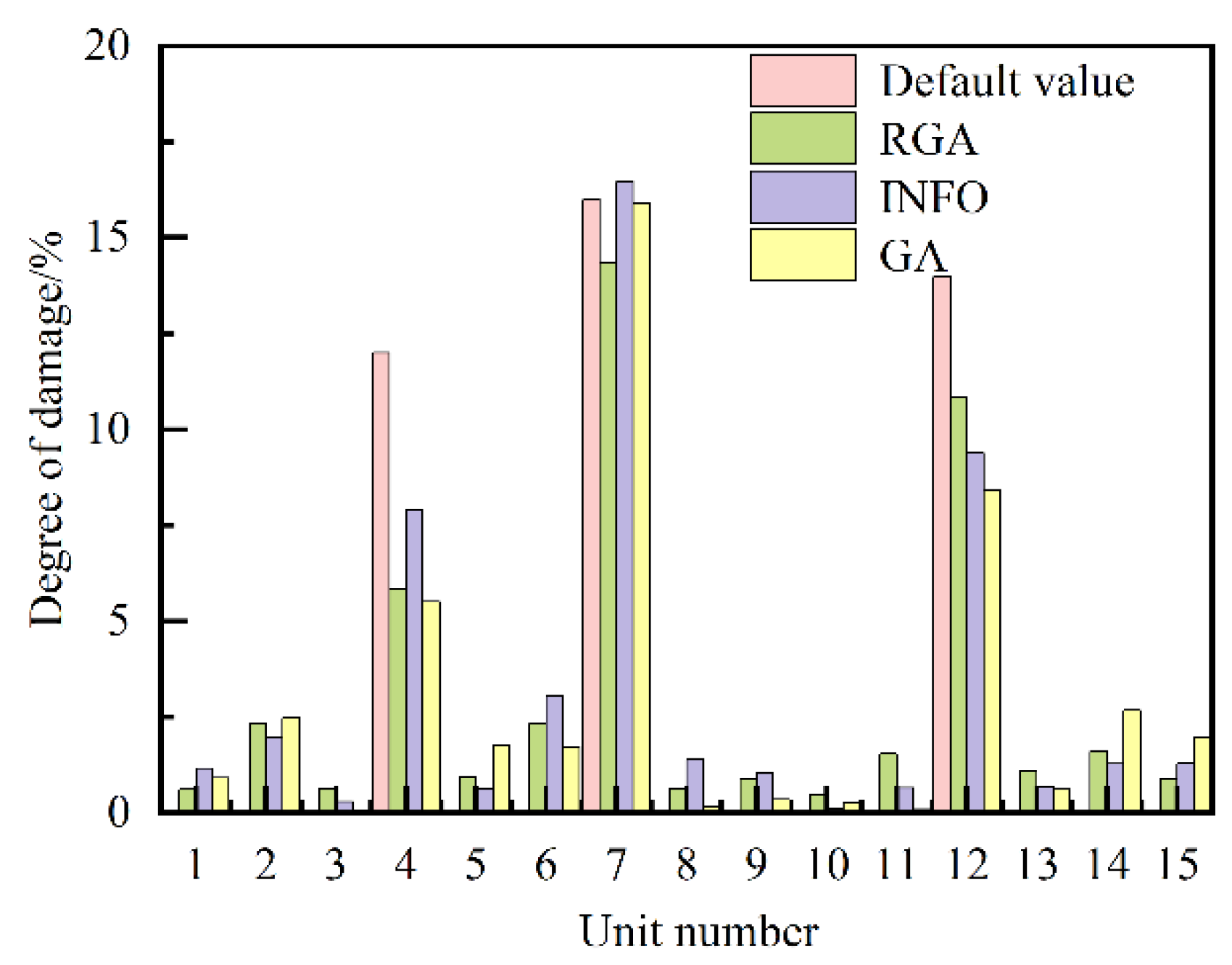
Adding 1%, 3% and 10% noise to the Case 4, the results of damage identification are shown in Figure 20, Figure 21, Figure 22 and Table 9, respectively.
From Figure 20, Figure 21 and Figure 22, it is observed that GA, RGA and INFO are able to accurately locate the damage position of the cantilever plate (Case 4) under 1% as well as 3% noise influence, under 3% noise, GA and RGA have more significant misjudgment at unit 2 and 6, while INFO has significant misjudgment at unit 2, under the influence of 10% noise, there are many obvious misjudgment units for the three methods.
Table 9 (Case 4) shows that under the influence of 1%, 3% and 10% noise, the mean errors of the target damage units identified by GA are 9.46%, 15.22% and 31.54%, by RGA are 8.38%, 13.19% and 28.17%, and by INFO are 1.40%, 5.78% and 23.32%, respectively, It can be seen that INFO has the highest accuracy in identifying the damage degree of the target unit, RGA has the second highest accuracy and GA has the lowest accuracy.
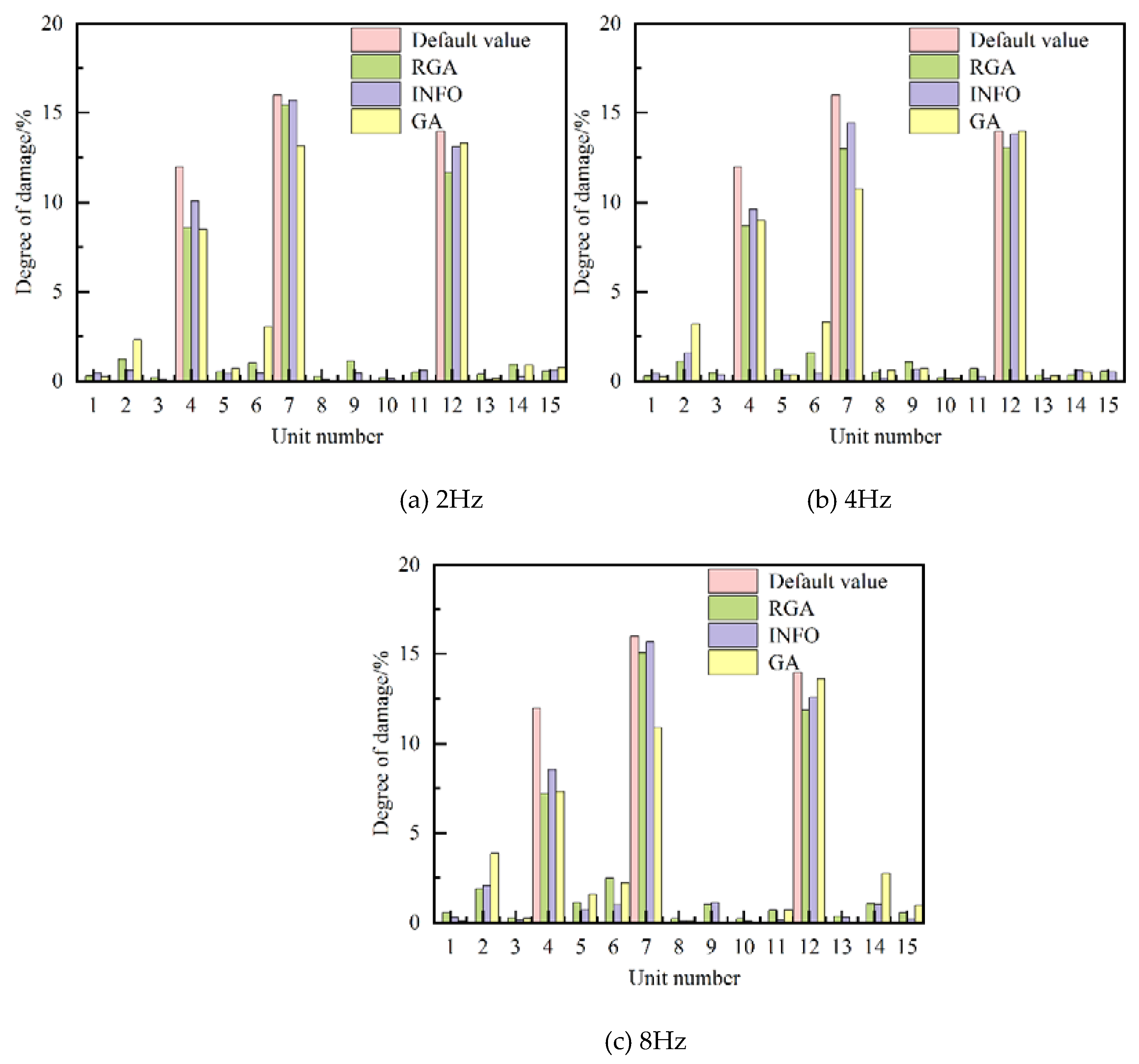
Keep the frequency range from 11Hz to 240Hz unchanged, the following three scenarios were simulated for the Case 4 of cantilever plate (adding 3% noise): (1) take points at equal intervals of 2Hz for a total of 115 frequency points. (2) take points at equal intervals of 4Hz for a total of 58 frequency points. (3) take points at equal intervals of 8Hz for a total of 29 frequency points. The damage identification results are shown in Figure 23, and the target damage unit identification results are shown in Table 10.
From Figure 23, it can be observed that under the influence of the same noise, the three algorithms can identify the damage location of the cantilever plate for three kinds of taking point spacing, and the three algorithms obtained the damage identification results of each plate unit at 2Hz spacing slightly worse than the results of the aforementioned Figure 21 at 1Hz spacing, but there is no obvious advantage in comparison with the identification results obtained at 4Hz spacing, while identification results for 4Hz spacing are better than those for 8Hz spacing.
Table 10 shows that, under the influence of the same noise, being equally spaced at 2Hz, the mean errors of the target damage units identified for the GA, RGA, and INFO are 17.34%, 16.08% and 7.95% , being equally spaced at 4Hz, are 19.26%, 17.67% and 10.31%, and being equally spaced at 8Hz, are 24.50%, 20.22% and 13.55% respectively. It can be seen that the identification accuracy of the three algorithms is getting lower and lower with the gradual increase of taking point spacing within the same frequency range. With the same taking point spacing, INFO has the highest identification accuracy, RGA has the second highest identification accuracy, and GA has the worse identification accuracy.

7. Conclusions

In this paper, RGA was obtained by improving GA with improved variation rate and crossover rate and non-uniform variation operator, which significantly improves its optimization ability, and INFO was first introduced as a high-performance optimization algorithm to identify the structure damage. Then the objective function based on dynamic response was established for each intelligent algorithm for damage identification by combining the finite element theory of structural dynamics, and the objective function balances the sensitivity of each part of the function to the damage through the weighting factors calculated by the damage classification. Finally, GA, RGA and INFO were respectively utilized in the numerical simulation to identify the damage cases of simply supported beams and cantilever plates with different levels of noise and different spacings of the frequency points. The simulations verify the effectiveness of the method and compare the effect of the algorithms for damage identification, and the following conclusions are obtained:
  • Under most of the same cases, INFO has the highest damage identification accuracy, RGA has the second highest identification accuracy, and GA has the lowest identification accuracy.
  • Under the same case, as the noise level gradually increases, the accuracy of damage identification of the algorithms will gradually become lower. Under the influence of 10% noise level, the three algorithms in the identification of multiple cases will appear obvious misjudgment units and the identification error of the damage degree of the target unit is larger, at this time the three algorithms can't accurately identify the damage cases.
  • In the same frequency range with the gradual increase in the frequency point spacing, the accuracy of damage identification for the algorithm gradually decreased, but part of the identification results is still within the acceptable range as the errors are not a significant increase.

References

  1. Qian C Y, Huang M S, Cheng S X, et al. Damage identification of the benchmark frame based on an improved cuckoo search[J]. Journal of Vibration and Shock, 2018, 37(22):158-163.
  2. Vaez S R H, Fallah N. Damage detection of thin plates using GA-PSO algorithm based on modal data[J]. Arabian Journal for Science and Engineering, 2017, 42(3):1251-1263. [CrossRef]
  3. Wan Z H, Huang M S, Cheng X H, et al. Two-stage damage identification method based on fractal theory and whale optimization algorithm[J], Advances in structural engineering, 2021, 21(12):1026-1058. [CrossRef]
  4. Mohan S C, Maiti D K, Maity D. Structural damage assessment using FRF employing particle swarm optimization[J]. Applied Mathematics and Computation, 2013, 219(20):10387-10400. [CrossRef]
  5. Miguel L F F, Lopez R H, Letícia F F M. A hybrid approach for damage detection of structures under operational conditions[J]. Journal of Sound and Vibration, 2013, 332(18):4241-4260. [CrossRef]
  6. Ding Z H, Huang M, Lu Z R. Structural damage detection using artificial bee colony algorithm with hybrid search strategy[J]. Swarm and Evolutionary Computation, 2016, 28:1-13. [CrossRef]
  7. Pan C D, Yu L, Chen Z P, et al. A hybrid self-adaptive Firefly-Nelder-Mead algorithm for structural damage detection[J]. Smart Structures and Systems, 2016, 17(6):957-980.
  8. Chen Z P, Yu L. A new structural damage detection strategy of hybrid PSO with Monte Carlo simulations and experimental verifications[J]. Measurement, 2018, 122:658-669. [CrossRef]
  9. Ding Z, Li J, Hao H. Structural damage identification using improved Jaya algorithm based on sparse regularization and Bayesian inference[J]. Mechanical Systems and Signal Processing, 2019, 132:211-231. [CrossRef]
  10. Guilherme F G, Sebastiao S C, Antonio C A. A sunflower optimization (SFO) algorithm applied to damage identification on laminated composite plates[J]. Engineering with Computers, 2019, 35(2):619-626. [CrossRef]
  11. Alkayem N F, Cao M, Ragulskis M. Damage localization in irregular shape structures using intelligent FE model updating approach with a new hybrid objective function and social swarm algorithm[J]. Applied Soft Computing, 2019, 83:105604. [CrossRef]
  12. Huang M S, Li X F, Lei Y Z, et al. Structural damage identification based on modal frequency strain energy assurance criterion and flexibility using enhanced Moth-Flame optimization[J]. Structures, 2020, 28:1119-1136. [CrossRef]
  13. Minh H L, Khatir S, Wahab M A, et al. An Enhancing Particle Swarm Optimization Algorithm (EHVPSO) for damage identification in 3D transmission tower[J]. Engineering Structures, 2021, 242:112412. [CrossRef]
  14. Li X L, Serra R, Olivier J. A multi-component PSO algorithm with leader learning mechanism for structural damage detection[J]. Applied Soft Computing, 2022, 116:108315. [CrossRef]
  15. Zhang G C, Wan C F, Xiong X B, et al. Output-only structural damage identification using hybrid Jaya and differential evolution algorithm with reference-free correlation functions[J]. Measurement, 2021, 199:111591. [CrossRef]
  16. Li Y F, Minh H L, Khatir S, et al. Structure damage identification in dams using sparse polynomial chaos expansion combined with hybrid K-means clustering optimizer and genetic algorithm[J]. Engineering Structures, 2023, 283:115891. [CrossRef]
  17. Thanh S T, Minh H L, Magd A W, et al. A new metaheuristic algorithm: Shrimp and Goby association search algorithm and its application for damage identification in large-scale and complex structures[J]. Advances in Engineering Software, 2023, 176:103363. [CrossRef]
  18. Muhammad I S, Samir K, Brahim B, et al. Damage assessment in laminated composite plates using modal strain energy and YUKI-ANN algorithm[J]. Composite Structures, 2023, 303:116272. [CrossRef]
  19. Holland, J. Genetic algorithms[J]. Scientific American, 1992, 267(1):66-73.
  20. Ahmadianfar I, Heidari A A, Noshadian S, et al. INFO: An efficient optimization algorithm based on weighted mean of vectors[J]. Expert Systems with Application, 2022, 195:116516. [CrossRef]
  21. Allemang R, J. The Modal Assurance Criterion (MAC): Twenty years of use and abuse[J]. Journal of Sound and Vibration, 2003, 37(8):14-23.
  22. Tong Z P, Zhang Y, Shen R Y, et al. Submarine finite element model updating method based on frequency response functions of vibration [J]. Journal of Shanghai Jiaotong University, 2005, 39(11): 111-114.
  23. Lu H, Feng Z R, Wang X J, et al. Structural damage identification based on hybrid whale annealing algorithm and sparse regularization[J]. Journal of Vibration and Shock, 2021, 40(17):85-91.
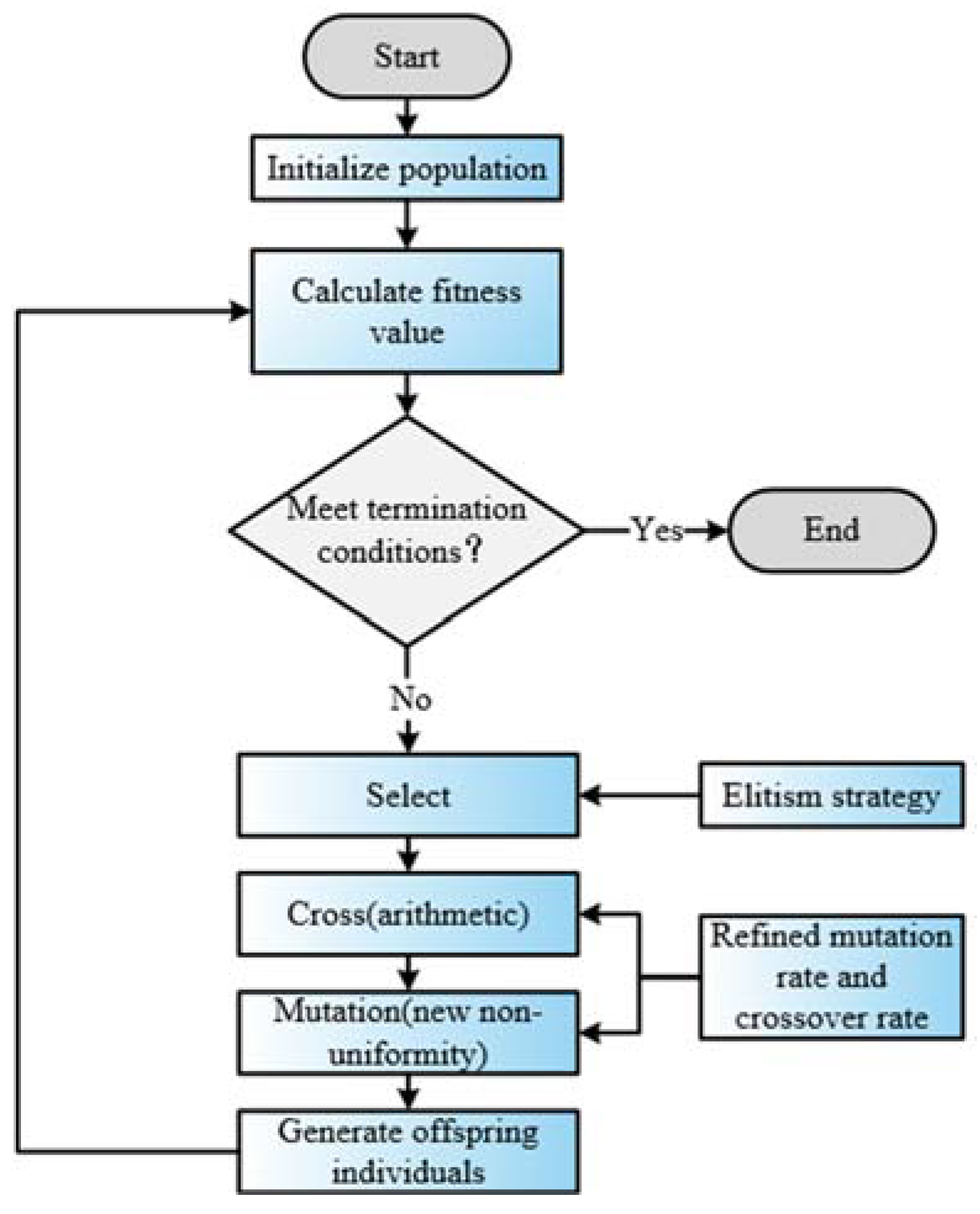
Figure 1. Flow of the RGA.
Preprints 116323 g001
Figure 2. Arithmetic crossover(2) Mutation.
Preprints 116323 g002
Figure 3. Flow of the INFO.
Preprints 116323 g003
Figure 4. Simulation model of simply supported beamTwo damage cases as shown in Table 1 are set up in the model. The symbol "#" in Table 1 and subsequent tables is used to connect the damage unit number with the damage degree of the unit.
Preprints 116323 g004
Figure 5. Damage identification results of each beam unit in Case 1 (no noise).
Preprints 116323 g005
Figure 6. Damage identification results of each beam unit in Case 2 (no noise).
Preprints 116323 g006
Figure 7. Damage identification results of each beam unit under 1% noise (Case 1).
Preprints 116323 g007
Figure 8. Damage identification results of each beam unit under 3% noise (Case 1).
Preprints 116323 g008
Figure 9. Damage identification results of each unit under 10% noise (Case 1).
Preprints 116323 g009
Figure 10. Damage identification results of each beam unit under 1% noise (Case 2).
Preprints 116323 g010
Figure 11. Damage identification results of each beam unit under 3% noise (Case 2).
Preprints 116323 g011
Figure 12. Damage identification results of each beam unit under 10% noise (Case 2).
Preprints 116323 g012
Figure 13. Damage identification results of each beam unit with different frequency spacing.
Preprints 116323 g013
Figure 14. Cantilever plate model.
Preprints 116323 g014
Figure 15. Damage identification results of each plate unit in Case 3 (no noise).
Preprints 116323 g015
Figure 16. Damage identification results of each plate unit in Case 4 (no noise).
Preprints 116323 g016
Figure 17. Damage identification results of each plate unit under 1% noise (Case 3).
Preprints 116323 g017
Figure 18. Damage identification results of each plate unit under 3% noise (Case 3).
Preprints 116323 g018
Figure 19. Damage identification results of each plate unit under 10% noise (Case 3).
Preprints 116323 g019
Figure 20. Damage identification results of each plate unit under 1% noise (Case 4).
Preprints 116323 g020
Figure 21. Damage identification results of each plate unit under 3% noise (Case 4).
Preprints 116323 g021
Figure 22. Damage identification results of each plate unit under 10% noise (Case 4).
Preprints 116323 g022
Figure 23. Damage identification results of each plate unit with different frequency point spacing.
Preprints 116323 g023
Table 1. Damage case settings for simply supported beam.
Damage case number Damage unit number#degree of damage/%
1 5 # 13, 9 # 9
2 3 # 19, 6 # 15, 10 # 15
Table 2. Identification results of target damage units for simply supported beam (no noise).
Damage case number Damage unit number # degree of damage/%
GA RGA INFO
1 5 # 12.80, 9 # 8.79 5 # 12.86, 9 # 8.90 5 # 13.00, 9 # 9.00
2 3 # 18.51, 6 # 15.34,
10 # 14.82
3 # 18.52, 6 # 15.19,
10 # 14.85
3 # 19.00, 6 # 15.00,
10 # 15.00
Table 3. Identification results of target damage units under three different levels of noise (Case 1).
Noise level/% Damage unit number # degree of damage/%
GA RGA INFO
1 5 # 12.13, 9 # 8.21 5 # 12.23, 9 # 8.36 5 # 12.61, 9 # 8.97
3 5 # 9.04, 9 # 9.26 5 # 11.44, 9 # 7.85 5 # 12.03, 9 # 8.74
10 5 # 2.75, 9 # 5.42 5 # 8.91, 9 # 4.92 5 # 9.76, 9 # 5.61
Table 4. Identification results under three different levels of noise (Case 2).
Noise level/% Damage unit number#degree of damage/%
GA RGA INFO
1 3 # 17.65, 6 # 16.18,
10 # 14.05
3 # 17.04, 6 # 15.25,
10 # 14.21
3 # 18.72, 6 # 15.07,
10 # 14.84
3 3 # 19.42, 6 # 17.08,
10 # 13.06
3 # 15.87, 6 # 14.56,
10 # 14.62
3 # 17.57, 6 # 15.22,
10 # 14.63
10 3 # 9.71, 6 # 18.01,
10 # 10.75
3 # 8.69, 6 # 14.51,
10 # 12.79
3 # 13.58, 6 # 16.17,
10 # 12.69
Table 5. Identification results with different frequency point spacing (Case 2).
Taking point spacing/Hz Damage unit number#degree of damage/%
GA RGA INFO
2 3#16.13, 6#17.07,
10#13.29
3#14.38, 6#15.42,
10#13.51
3#17.47, 6#15.54,
10#13.93
4 3#15.46, 6#17.16,
10#12.85
3#14.24, 6#15.50,
10#13.35
3#18.40, 6#15.62,
10#13.18
8 3#14.39, 6#18.20,
10#12.34
3#12.45, 6#15.61,
10#12.97
3#16.89, 6#15.33,
10#13.37
Table 6. Damage case settings for cantilever plate.
Damage case number Damage unit number # degree of damage/%
3 2 # 18, 10 # 13
4 4 # 12, 7 # 16, 12 # 14
Table 7. Identification results of target damage units for cantilever plate (no noise).
Case number Damage unit number # degree of damage/%
GA RGA INFO
3 2#16.54, 10#12.02 2#16.32, 10#12.35 2#18.00, 10#13.00
4 4#11.36, 7#15.47,
12#14.20
4#11.48, 7#15.35,
12#13.87
4#12.00, 7#16.00,
12#14.00
Table 8. Identification results of target damage units of cantilever plate under three different levels of noise (Case 3).
Noise level/% Damage unit number#degree of damage/%
GA RGA INFO
1 2#15.43, 10#11.17 2#14.94, 10#11.89 2#17.37, 10#12.70
3 2#12.62, 10#9.44 2#12.87, 10#10.46 2#16.37, 10#12.41
10 2#5.12, 10#6.06 2#7.45, 10#7.01 2#7.38, 10#8.80
Table 9. Identification results of target damage units of cantilever plate under three different levels of noise (Case 4).
Noise level/% Damage unit number#degree of damage/%
GA RGA INFO
1 4#10.73, 7#17.18,
12#12.54
4#10.65, 7#15.09,
12#12.85
4#11.70, 7#15.91,
12#13.83
3 4#9.29, 7#14.41,
12#12.16
4#9.20, 7#14.91,
12#12.68
4#10.80, 7#15.18,
12#13.69
10 4#5.51, 7#15.89,
12#8.42
4#5.83, 7#14.34,
12#10.82
4#7.91, 7#16.46,
12#9.38
Table 10. Identification results of target damage units of cantilever plate with different frequency point spacing (Case 4).
Taking point spacing/Hz Damage unit number#degree of damage/%
GA RGA INFO
2 4#8.48, 7#13.16,
12#13.31
4#8.62, 7#15.45,
12#11.67
4#10.10, 7#15.71,
12#13.13
4 4#8.99, 7#10.78,
12#14.01
4#8.68, 7#13.02,
12#13.06
4#9.62, 7#14.43,
12#13.82
8 4#7.34, 7#10.89,
12#13.62
4#7.21, 7#15.08,
12#11.90
4#8.57, 7#15.68,
12#12.59
Disclaimer/Publisher’s Note: The statements, opinions and data contained in all publications are solely those of the individual author(s) and contributor(s) and not of MDPI and/or the editor(s). MDPI and/or the editor(s) disclaim responsibility for any injury to people or property resulting from any ideas, methods, instructions or products referred to in the content.
Copyright: This open access article is published under a Creative Commons CC BY 4.0 license, which permit the free download, distribution, and reuse, provided that the author and preprint are cited in any reuse.
Prerpints.org logo

Preprints.org is a free preprint server supported by MDPI in Basel, Switzerland.

Subscribe

© 2024 MDPI (Basel, Switzerland) unless otherwise stated