A Strategy of Weak-Connected Grid Search for Noise Filtering and Density Grid-Based Data Clustering

Preprint

Article

A Strategy of Weak-Connected Grid Search for Noise Filtering and Density Grid-Based Data Clustering

Altmetrics

Downloads

Views

Comments

This version is not peer-reviewed

Submitted:

28 August 2024

Posted:

28 August 2024

You are already at the latest version

Alerts

Abstract

One of the efficient data mining tools is density-based clustering, including the density grid-based clustering. However, a common drawback always existing in clusters made by the density grid-based method is the existence of weakly connected grids deriving mainly from noise. Appearing such an unwanted connection with a high frequency reduces the accuracy of the obtained cluster data space (CDS) and its application efficiency. Here, we present an essential improvement to overcome this problem. First, we describe a concept of the weak-connected grid cell (WCG) and present a fuzzy-type approximation to depict the density-based distribution of data points at grid nodes. Then, we propose a strategy of searching WCG for density grid-based clustering (SWCG-DGB) to set up a CDS, filter noise, and tune the created CDS. A buffer is deployed during this phase to collect border points and filter noise, which improves the computational time significantly, especially for noisy datasets. Results from numerical surveys reflected the compared efficiency of this method in clustering validity, including the accuracy of the number of clusters.

Keywords:

Subject: Engineering - Mechanical Engineering

1. Introduction

The characteristic analysis is a significantly concerning aspect in various fields, such as geology, medicine, business, or engineering systems, including image and data processing [1,2]. To be seen as a vital tool for characteristic analysis, clustering explores the data structure and distills meaningful information via analyzing, separating, and merging similar data points into distinct groups. There have been many clustering approaches, each one owning its specific techniques [3,4,5]. Among them, density-based clustering is one of the most famous paradigms [6,7,8,9].

In [6], Martin Ester et al. presented Density-Based Spatial Clustering of Applications with Noise (DBSCAN). It finds data points in a circle of radius ε and adds them into a cluster of data points with the same characteristic. If the number of neighbors of an unassigned point is less than a predefined threshold minPts, the point is seen as noise. Its considerable benefit is the ability to merge data points into arbitrary-shaped clusters without any assumption about the number of data clusters. This aspect is necessary and vital to face an inevitable characteristic of large data sets in real applications [10,11]. It is the advantage of most density-based methods. However, using Euclidean distance in most algorithms results in computational complexity, especially for large datasets [12]. Inefficiencies when dealing with severely noisy datasets are also a common problem of density-based clustering, including the method shown in [6]. Over recent years, many different methods have been proposed deriving from efforts to extend the ability of density-based methods [13,14,15]. Also, several combinations of private approaches have been considered to form more efficient methods, such as the collaboration of density-based and grid-based clustering solutions [13,16,17,18,19,20,21,22]. The GRIDBSCAN [13] is a development of the DBSCAN based on the grid approach to provide a solution to different densities that DBSCAN cannot overcome. It follows three phases. The first one selects appropriate grids for homogeneous density in each grid. The second one merges cells with similar densities and recognizes the most suitable values as ε and minPts to run the DBSCAN with these identified constants in the third phase. Even though getting the compared advantages in terms of accuracy of the generated CDS, the high time-consuming and matching with small-sized databases only are its considerable disadvantages.

To solve the above issues partly, the HDBSCAN [16,17], DPC [18], and DPCSA [19] considered sophisticated density-based approaches. As an extension of the DBSCAN, the HDBSCAN [16] presented a multiple clustering in a hierarchy to get the best possible solution. It took minPts as input and employed a non-parametric density estimation method followed by Hartigan’s notion of hard clusters to create a simplified cluster tree to obtain the final solution for an unlimited range of density thresholds. For the DPC [18], it was a density-based clustering via the density-peak clustering approach to determine the optimal number of clusters in a dataset. The idea behind this strategy is that the cluster centers have larger densities and that the distances between them are significant. The method, however, is dependent on user input due to the manually selected center points from the decision graph. Yu et al. expanded the DPC by proposing the DPCSA [19]. It used a two-stage cluster label assignment to data points to reduce error propagation. By using a dynamic closest neighbor table update approach, the DPCSA overcomes the constraints of DPC and improves clustering performance. However, a user still needs to select the cluster centers from the decision graph.

Recently, a fast-density grid-based method (DGB) was presented in [20] with the improvement of computational time. This method proposes a type of density computation that has rarely been found in convenient algorithms before. Instead of calculating the density of grid cells as the famous algorithms like ENCLUS [21], CLIQUE [22], or DSTREAM [23], it would compute the density of grid nodes only without considering that at each data point in the cells. There is no need to calculate the Euclidean distances between mutual data points to improve the computational complexity. However, like to the traditional density grid-based clustering methods, the challenge of misclassification caused by incorrectly recognizing the number of clusters may usually exist.

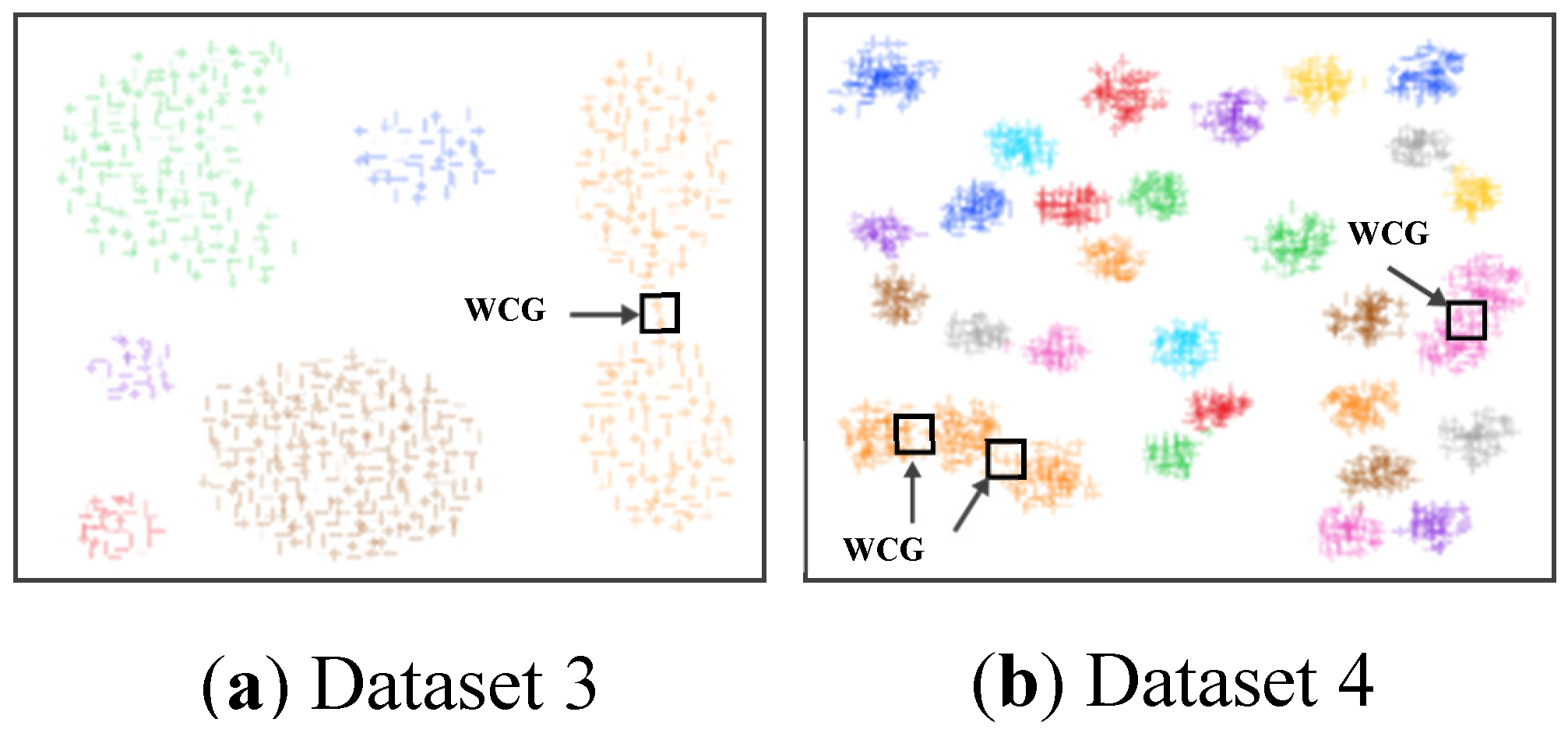
It can observe that density grid-based clustering owns promising advantages. However, the limitations mentioned above blur its effectiveness. Especially, the existence of noise may cause weak links between some grids that make the obtained results unstable and inaccurate. Focusing on this aspect, we propose a Density Grid-Based Clustering algorithm named SWCG-DGB using a strategy of Weak-Connected Grid search. First, we suggest a concept called Weak-Connected Grid Cell (WCG), by which we describe outside grids, neighboring grids, and a buffer. A fuzzy type approximation [24,25] is then employed to calculate the density of grid nodes for establishing initial clusters. A search strategy is carried out to seek and remove WCG existing in the initial clusters. As a result, Density Grid-Based data clusters are finally generated in the filtered data space. As usual, simulation surveys are performed to evaluate the SWCG-DGB. Our main contributions are as follows:

We point out a common drawback often appearing in the density grid-based clustering approach related to the WCG. Accordingly, we propose a solution for improving the clustering validity, including filtering noise and fine-tuning the generated CDS.
We propose a buffer for storing features of data points and the grid-cell’s coordinates. It allows detecting WCGs more effectively with a lower computational cost. The reason is that only the data points marked in the buffer are indicated as border or noise points instead of the entire dataset. This enhancement is very efficient for large datasets.

The rest of the paper is organized as follows. The related concepts are presented in Section 2 to depict the SWCG-DGB in Section 3. The following section shows surveys and evaluations via benchmark datasets. Finally, Section 5 gives the vital conclusions of this approach.

2. Related Concepts

Definition 1.

(Characteristic Vector). The characteristic vector is a tuple (pos, C, mark) created by a structure type table. Here, pos is the position of grid cells (or cells for short), C is a set of data points in the same cell, and mark is the number of clusters marked for all cells in the cluster matrix.

Definition 2.

(Neighboring Cells). A cell is a neighbor of another one if both have at least one common boundary.

Let’s consider two cells

g_{1} (j_{1}^{1}, j_{2}^{1}, ..., j_{k}^{1})

and

g_{2} (j_{1}^{2}, j_{2}^{2}, ..., j_{k}^{2})

in a k-dimension data space. Where

(j_{1}^{1}, j_{2}^{1}, ..., j_{k}^{1})

and

(j_{1}^{2}, j_{2}^{2}, ..., j_{k}^{2})

are the ordinal numbers on two different data dimensions. We follow the standard grid concept, to which the distance between any two neighboring nodes on an arbitrary data dimension is one. Accordingly, in general, g₁ and g₂ are neighbors (or neighboring cells, denoted g₁ ~ g₂) if the two conditions in (1) must be satisfied:

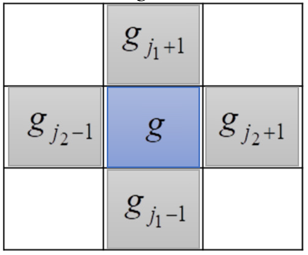
\begin{array}{l} 1) j_{i}^{1} = j_{i}^{2}, \\ 2) |j_{d}^{1} - j_{d}^{2}| = 1, i, d = 1 ... k and d \neq i . \end{array}

(1)

Figure 1 shows the neighboring cells of cell g in the two-dimension data space

Definition 3.

(Grid Cluster and Outside Grid) [23]. A set of cells

G = (g_{1}, ..., g_{m})

is a grid cluster (or a cluster for short) if for any two cells

g_{i}, g_{j} \in G

, there exist a sequence of cells

g_{d_{1}}, ..., g_{d_{h}} \in G

such that

g_{d_{1}} \equiv g_{i}

g_{d_{h}} \equiv g_{j}

, and

g_{d_{1}} \sim g_{d_{\begin{array}{l} 2 \end{array}}}

g_{d_{2}} \sim g_{d_{\begin{array}{l} 3 \end{array}}}

,…, and

g_{d_{h - 1}} \sim g_{d_{\begin{array}{l} h \end{array}}}

. Consider

g_{k} \in G

, if g_k has at least one neighbor not belonging to G, then g_k is outside grid in G.

Definition 4.

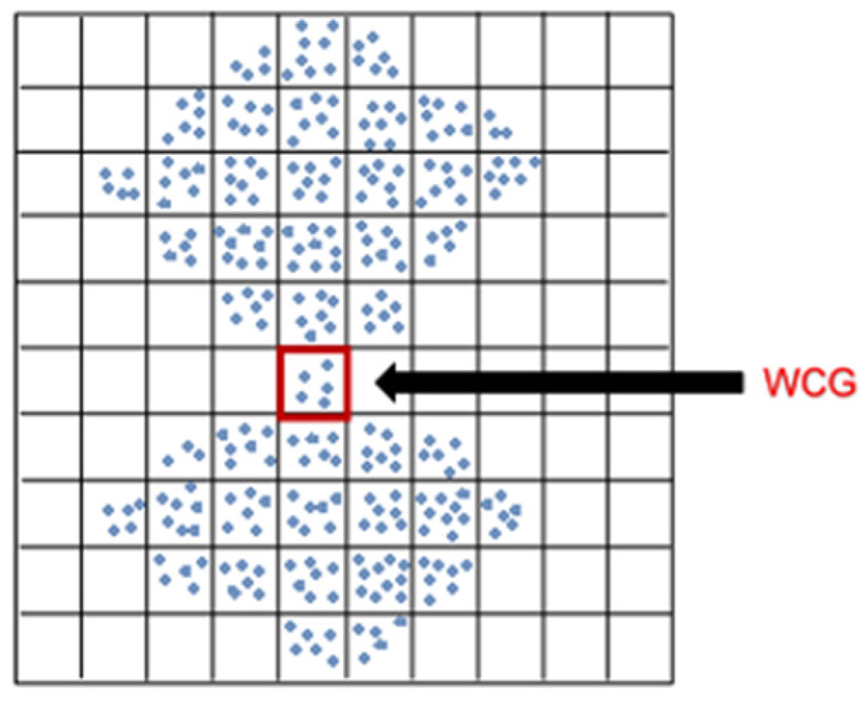
(Weak-Connected Grid Cell, WCG). Let’s consider a cell in a certain cluster. The cell is a WCG if both of the following statements are satisfied. 1) On one arbitrary data dimension, two neighbors of this cell belong to this cluster; and 2) Two of its neighbors on any of the remaining data dimensions do not belong to this cluster.

Figure 2 illustrates a WCG existing in a cluster. In this case, the cluster may be split easily into two smaller ones at this WCG. For our algorithm, the first separation step makes a rough space of initial clusters. This observation takes the role of a direction for the next phase: fine separation. The next section details these aspects.

Definition 5.

(Fuzzy Type Approximation). Let’s consider data point P on the d-th data dimension of a normalized k-dimension data space. A fuzzy membership is defined as follows:

f_{d} (N_{d}) = \{\begin{cases} 1 - Δ_{d}, i f Δ_{d} \leq λ \\ 0, o t h e r w i s e \end{cases}

(2)

where, λ is the length of each cell,

Δ_{d} = |P_{d} - N_{d}|

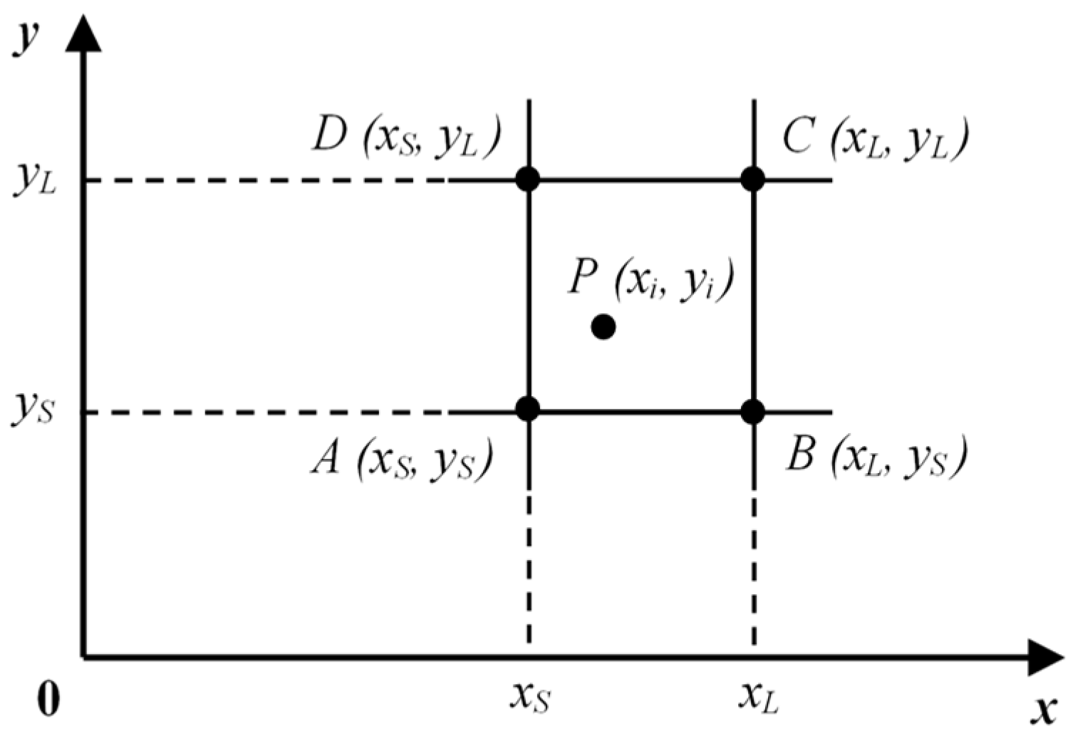
, P_d is the coordinate of P, and N_d is the node’s coordinate in d-th dimension (see Figure 3).

In Figure 3, x_S and x_L (y_S and y_L) are two coordinates on the x-axis (y-axis), signed x_Small and x_Large (y_Small and y_Large), respectively. Points A, B, C, and D are four nodes of the cell containing P. The density of these nodes is calculated, and node C (x_L, y_L), which is the representation of data point P, is merged into the struct_table type buffer.

Be noted that the distance between any two neighbor nodes in the standard grid (λ) equals one. Equation (2) shows the contribution of each data point to its surrounding nodes and is utilized to calculate the local density of the nodes according to one data dimension. In the n-dimensional data space, the node density is therefore calculated:

W = \prod_{d = 1}^{n} f_{d} (N_{d})

(3)

For example, for data point P(x_i,y_i) in Figure 3, the weighted fuzzy densities to four nodes A, B, C, and D are

W_{A} = (1 - |x_{i} - x_{S} (A)|) (1 - |y_{i} - y_{S} (A)|)

(4)

W_{B} = (1 - |x_{i} - x_{S} (B)|) (1 - |y_{i} - y_{S} (B)|)

(5)

W_{C} = (1 - |x_{i} - x_{S} (C)|) (1 - |y_{i} - y_{S} (C)|)

(6)

W_{D} = (1 - |x_{i} - x_{S} (D)|) (1 - |y_{i} - y_{S} (D)|)

(7)

The node’s local density is applied by summing up the density of all the variables according to (Equations 4-7):

Δ_{A} = \frac{W_{A} d_{p}}{W_{A} + W_{B} + W_{C} + W_{D}}

(8)

Δ_{B} = \frac{W_{B} d_{p}}{W_{A} + W_{B} + W_{C} + W_{D}}

(9)

Δ_{C} = \frac{W_{C} d_{p}}{W_{A} + W_{B} + W_{C} + W_{D}}

(10)

Δ_{D} = \frac{W_{D} d_{p}}{W_{A} + W_{B} + W_{C} + W_{D}}

(11)

dp is the density of data point P, which is set to 1 in the general case to simplify the defuzzification process (8)-(11) because the denominator in these equations would always be one

W_{A} + W_{B} + W_{C} + W_{D} = 1

(12)

Definition 6.

(Density Matrix). The density_matrix keeps the density of nodes. It has the size to be square of no_grid, which is the size of the grid in each dimension.

In the beginning, the density of all nodes is computed via equations (2-11) and stored in the density_matrix. It is then used for the mountain ridge searching process by finding the nodes with a density higher than a density threshold. The nodes owning a density value less than this threshold are marked as zero-density nodes. Hence, instead of processing all the nodes, one only needs to operate on a small number of nodes with non-zero density to accelerate the speed of the clustering process.

3. Proposed Method

Section 1 mentioned some typically density-based clustering methods, such as the DBSCAN [6], HDBSCAN [16], DPC [18], DPCSA [19], and DGB [20]. Despite owning advantages in fast computation, they have a misclassification when finding the number of data clusters in many cases related to WCGs. Here, we present the algorithm SWCG-DGB for density-based clustering with a proposed solution for the above difficulty. It is an extension of the DGB [20] with a supplemented vital tool for finding WCGs to filter noise, make an initial CDS, and perform fine-tuning of the CDS. Let’s consider a given source dataset. The main steps of the SWCG-DGB are as follows.

3.1. Initialization

It consists of normalizing the data space, finding the corner coordinates of each data point to map the data point into the buffer, and calculating the local density of nodes.

We normalize the original dataset to [0, 1], and then each data point is scaled into a grid range of [1, no_grid]. Where, no_grid is the size of the grid in each dimension. In other words, it is the number of cells in each data dimension. Here, we select

n o_g r i d = N \in N *

for all the data dimensions. As an example, with any data point P(x_i,y_i) in Figure 3, the normalization takes place as:

x_{i} \leftarrow \frac{(x_{i} - x_{\min})}{x_{\max} - x_{\min}} (N - 1) + 1

(13)

y_{i} \leftarrow \frac{(y_{i} - y_{\min})}{y_{\max} - y_{\min}} (N - 1) + 1

(14)

where x_min (y_min) and x_max (y_max) respectively are the minimum and maximum values of the dataset in x-dimension (y-dimension).

With each normalized data point, calculating local density for four nodes is done by Equations (8-12) using the fuzzy type approximation mentioned in Definition 5. These densities are saved in different local matrices, and then the sum of local density matrices is stored in a matrix named density_matrix with an initial setting to be zero.

3.2. Finding the Number of Clusters

Finding mountain ridges (or initial clusters) is a core process for the SWCG-DGB. In this progress, we map data points onto individual data clusters and store the information in a cell array named CL_set. Algorithm 1 depicts this process. First, from the density of nodes sorted in descending order, the highest density is chosen for the mountain ridge searching task. Then, for each mountain ridge, its neighboring nodes whose density is higher than a threshold set up prior are merged into it. The mapping of data points into suited clusters happens regularly.

Algorithm 1. Searching mountain ridges

Inputs: All data points.
Outputs: The updating position of the node in the buffer and CL set.
1: Calculating density of nodes and add them into density_matrix
2: Reshaping density_matrix, finding the node_i has max_density
3: while (max_density > edge_factor )
4:   for i =1 to length(k) of high_density_nodes set
5:      (x_i, y_i)=get_position(row_i, col_i)
6:      cluster_matrix(row_i, col_i)=n (no_cluster)
7:      updating node(x_j, y_j) into the buffer and CL_set
8:      for m =k+1 to length of (no_grid*no_grid)
9:      if (density of node_m > edge_factor)
10:        (x_m, y_m)=get_position(row_m, col_m)
11:        if (node(x_m, y_m) is neighbor of node(x_i, y_i) )
12:           cluster_matrix(row_m, col_m) = cluster_matrix(row_i, col_i)
13:              density_matrix(row_m, col_m)=max_density
14:              high_density_nodes=[high_density_nodes m]
15:              updating node(x_m, y_m) into the buffer and CL_set
16:        end (if 11)
17:      end (if 9)
18:   end (for 8)
19: end (for 4)
20:   high_density_nodes=[1]; n=n+1
21: end (while 3)

In this algorithm we select a density threshold for finding the first mountain ridge. It is the maximal density of random grid cells arranged in density_vector. Then we get the position of this cell and assign it the corresponding location in cluster_matrix equals no_cluster (n), which is the name of the cluster and was set one in the first stage. After that, we examine the position of the next cell in the density_matrix and get the cells’ position. It is done if it has a high enough density. As a result, the neighbors of those cells contain nodes satisfying the edge_factor threshold condition, which is a ratio of the prior maximum peak density value. The value of the edge_factor parameter is inferred in the initial step based on the characteristics of each dataset. Simultaneously, we tune the grid ratio value to obtain clustering results. Besides, merging and marking these cells’ data points into the buffer and mapping them onto CL_set are conducted. This process establishes core clusters containing most of the source data points in cells that are the high-density areas.

3.3. Searching the Weak-Connected Grids

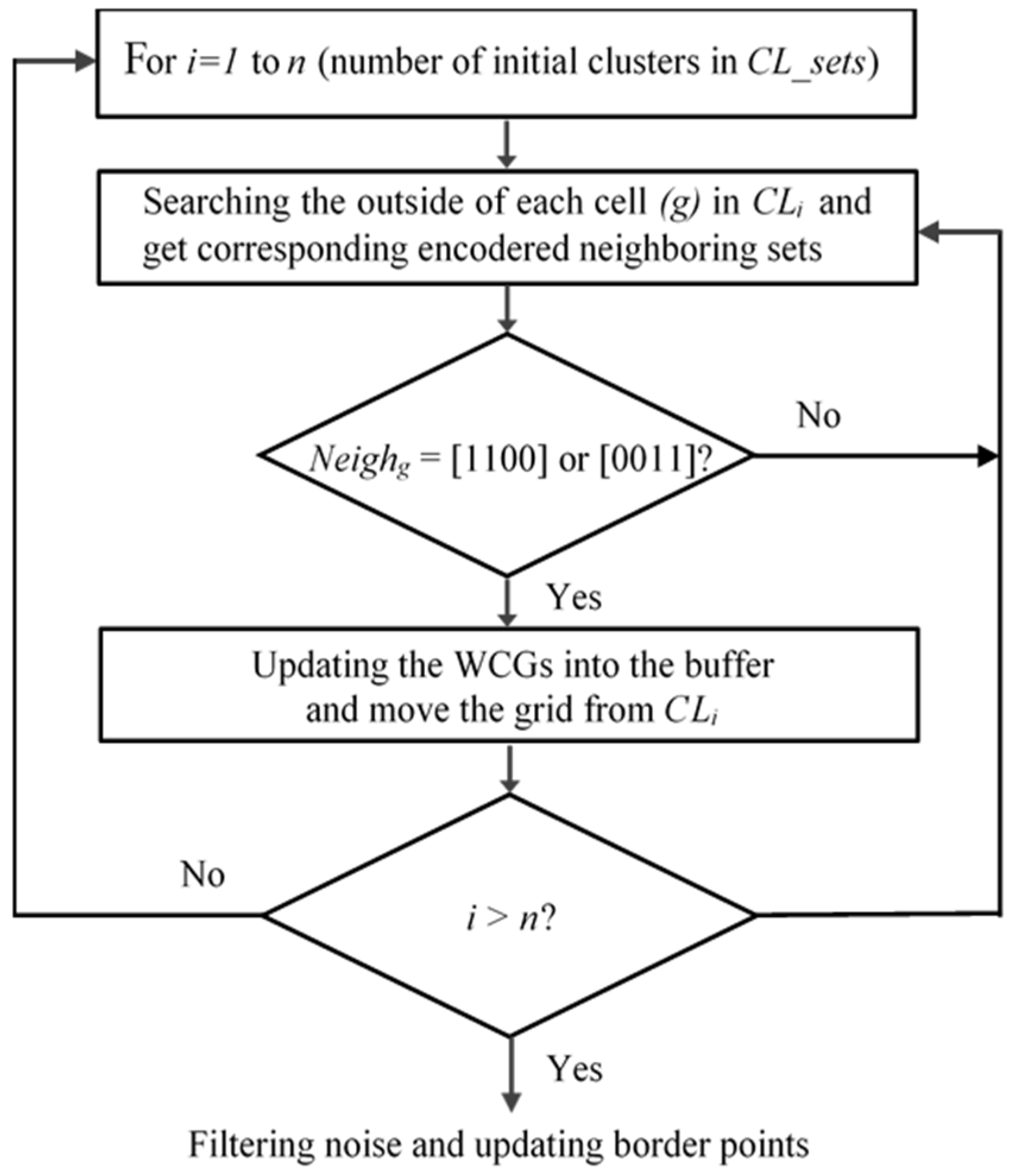
Searching for WCGs is a meaningful development in our algorithm. With every cluster formed and located in CL_set, we search for the WCGs inside it. One thing noted in this process is that after finding out the WCGs, we do not delete data points inside but just move and mark them into the buffer as a zero-number, which are called zero_marked_data. These data will be reclassified and returned to those clusters. This essential work ensures the maximum avoidance of data loss. The workflow for searching the WCGs is in Figure 4.

In the above process, outside grids are searched in each cluster and then we check the order of neighboring grids in terms of binary code. An outside grid is a WCG if its encoded neighboring set is [1 1 0 0] or [0 0 1 1]. In other words, an outside grid is a WCG if it has two neighbors on the same dimension located in the same cluster and the other neighbors are not in this cluster. When the WCG is found, data points in it are moved from the cluster and marked with a zero-number in the buffer for filtering noise and updating border points in the next part. The following work is to get the position of WCGs and mark them in the density_matrix for splitting big clusters into smaller clusters separately. The search for the WCGs is depicted in Algorithm 2 below.

Algorithm 2. Searching WCGs

Input: All grids on the CL set.
Output: Detecting and moving the WCGs out of each CL set.
1: for i =1 to length_of CL_set
2: for m =1 to length_of CL_i
3:    if grid_m is outside of CL_i
4:    [Neigh_m]= get_neighbors of grid_m
5:    if Neigh_m =[0; 0; 1; 1] or [1; 1; 0; 0]
6:        marking data points of (grid_m) as noise in buffer
7:        moving data points of (grid_m) out of CL_i
8:        (x_m, y_m)=get position of (grid_m) from buffer
9:        density_matrix (row_m, col_m) = 0
10:    end (if 5)
11:      end (if 3)
12: end (for 2)
13: end (for 1)

3.4. Filtering Noise and Updating Border Points

Algorithm 3 below describes the progress for filtering noise and updating border points. In the finding of mountain ridges presented in the above section, the border nodes are detected via setting a threshold that is the edge_factor parameter for identification of mountain ridges and border points. From the noise_threshold set up via the initial parameter function, nodes whose local density is smaller than the threshold are considered noise.

Algorithm 3. Filtering noise and updating border points

Input: All points of zero-number_grid set in buffer.
Output: Removing noise and updated border points in obtained clusters.
1: for i =1 to length of zero-number_grid set in buffer
2:   get_position(row_i, col_i);
3:   if ( cluster_matrix(row_i, col_i)=0 and
  density_matrix (row_i, col_i) > noise_threshold )
4:         for k=1 to 4
5:            if cluster_matrix (node_k) > 0
6:             satisfactory_node = satisfactory_node+1;
7:             sum = sum(satisfactory_node);
8:            end (if 5)
9:         end (for 4)
10: end (if 3)
11: if sum = 1, get density of satisfactory node
12:       if node_ density <noise_threshold
13:          cluster_matrix (row_i, col_i)=0;
14:            grid_i = noise; break;
15:       else
16:            move grid_i to corresponding cluster;
17:       end (if 12)
18: end (if 11)
19: if sum > 1, get total density of satisfactory nodes
20:       if total node_ density <noise_threshold
21:          cluster_matrix (row_i, col_i)=0;
22:            grid_i = noise; break;
23:       else
24:            move grid_i to corresponding cluster;
25:       end (if 20)
26: end (if 19)
27: end (for 1)

Be noted that the buffer for storing and marking the original data set above-mentioned makes finding noise and updating border points convenient. Instead of searching for all data points in the entire data set, we only handle data points marked zero that does not belong to any arbitrary cluster. It allows for speeding up the process, which is vital for real datasets in real-world applications, especially data streams changing over time.

The entire progress of SWCG-DGB is presented by Algorithm 4.

Algorithm 4. The SWCG-DGB

1: Normalizing each data point P(x_i,y_i) following equations (13) and (14).
2: Calculating corner coordinates of each data point P(x_i,y_i) and update C(x_L, y_L) into the buffer.
3: Calculating the local density of nodes following equations (4)-(7) and add them into the density_matrix.
4: Finding the mountain ridges (or initial clusters) and map data points corresponding to these clusters into CL_sets (Algorithm 1).
5: Searching the Weak-Connected Grids (Algorithm 2).
6: Filtering Noise and Updating Border Points (Algorithm 3).

4. Experimental Simulation

4.1. Approach

As usual, the accuracy of the quantified cluster number (QCN) is the coinciding degree between the QCN and the actual (‘right’) number of clusters (RNC). The reasonableness in the distribution of samples in the created cluster space reflects clustering validity. In addition, one often considers calculating time (CT) in actual applications. As a result, the higher the accuracy of QCN and the clustering validity degree along with the lower the CT, the higher the clustering effectiveness. In this section:

We utilize Rand Index (RI) [27], Adjusted Rand Index (ARI) [28] and Normalized Mutual Information (NMI) [29] to quantify the clustering validity. All these clustering validity indexes belong to [0, 1], and their higher values represent better clustering results;
The RNC is visually observed to estimate the accuracy.

Based on the above direction in evaluating, we compare the proposed SWCG-DGB method with the five other density-based clustering methods discussed in Section 1, namely DBSCAN [6], HDBSCAN [16], DPC [18], DPCSA [19], and the density grid-based clustering method, DGB [20]. The two HDBSCAN and DBSCAN need user input parameters. Hence, we try to specify the best values of their parameters before the surveys. To benefit DPC and DPCSA, the detected number of clusters is adjusted to the correct number of classes in accordance with the decision graph. Due to the DGB and SWCG-DGB not needing any input parameter, we carry out surveys with similar no_grid values. Accordingly, we set up their parameters as in Table 2.

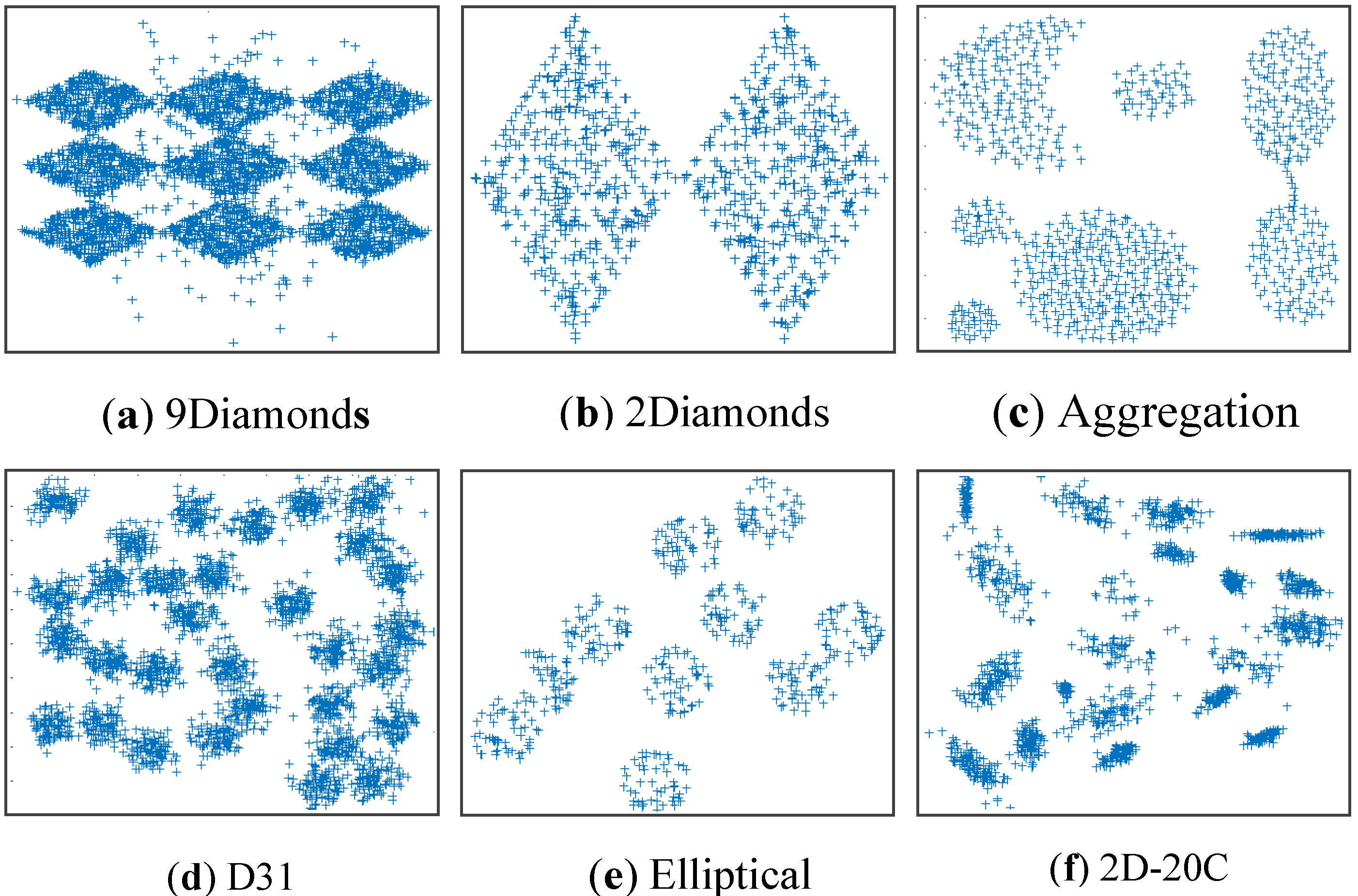
We employ six 2-dimensional synthetic datasets with the pre-observed RNC detailed in Table 1 and Figure 5 to evaluate the SWCG-DGB. These datasets are commonly used as benchmarks to test (https://github.com/deric/clustering-benchmark). The surveys are on MATLAB R2019a under the Windows 10, 64-bit operating system, Intel (R) Core (TM) i5-1135G7 @ 2.40 GHz, 16GB RAM.

4.2. Evaluation Measures

The accuracy of the quantified cluster number (QCN) is evaluated via visualization and the calculating time (CT) are compared. For a given synthetic dataset, the target is to seek QCN such that QCN is equal to its RNC with a CT as low as possible. Besides, Rand Index (RI), Adjusted Rand Index (ARI) and Normalized Mutual Information (NMI) are employed to estimate the performance of comparing algorithms. Both of their values are in [0, 1]. And better clustering performance is indicated by higher values for them.

The RI [27] is a measure to compare the output of a clustering algorithm with actual clusters. This measure may also be used for comparing the results of two clustering methods. RI is described as follows:

R a n d I n d e x (X, C) = \frac{(a + b)}{\frac{n}{2}}

(15)

In (15), n is the total number of samples, X and C represent two distinct sets of clusters, and a and b represent the number of pairs of samples that belong to (non-similar) distinct groups in X and C, respectively.

Another measure is the ARI [28] that is used to assesses the clustering results via assuming a generalized hypergeometric distribution as the model of randomness. This measure is presented as follows:

A R I (X, C) = \frac{\sum_{i j} (\frac{n_{i j}}{2}) - \sum_{i} (\frac{a_{i .}}{2}) \sum_{j} (\frac{b_{i .}}{2}) / (\frac{n}{2})}{\frac{1}{2} [\sum_{i} (\frac{a_{i .}}{2}) \sum_{j} (\frac{b_{i .}}{2})] - \sum_{i} (\frac{a_{i .}}{2}) \sum_{j} (\frac{b_{i .}}{2}) / (\frac{n}{2})}

(16)

where X is the results and C denotes the actual labels. n_ij is the number of samples same in both clusters x_i and

c_{i}

, a_i and b_i are respectively the number of the same samples of x_i and c_i clusters.

Finally, NMI [29] is a widely employed metric to evaluate clustering approaches. The following definition, this metric is applied information theory to quantify the differences between two clustering partitions, is:

N M I (X, C) = \frac{M I (X, C)}{\sqrt{H (X) H (C)}}

(17)

In the above, Mutual Information (MI) achieves the degree of information between the two random variables and is defined in (18).

M I (X, C) = \sum_{x_{i} \in X, c_{i} \in C} p (x_{i}, c_{i}) l o g (\frac{p (x_{i}, c_{i})}{p (x_{i}) p (c_{i})})

(18)

where p(x_i,c_i) is the probability of belonging an instance to clusters x_i and c_i at the same time. Additionally, p(x_i) and p(c_i) are the probabilities that an instance will belong to associated clusters x_i and c_i, respectively. Take note that NMI takes its values between 0 and 1. It takes the value of 1 if two clusters are precisely similar, and it takes the value of 0 if two clusters are independent.

4.3. Simulating Results on Synthetic Datasets

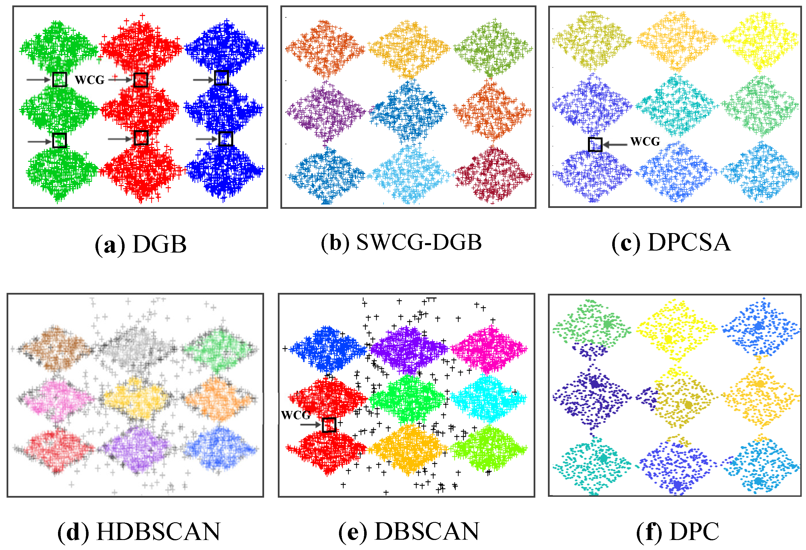
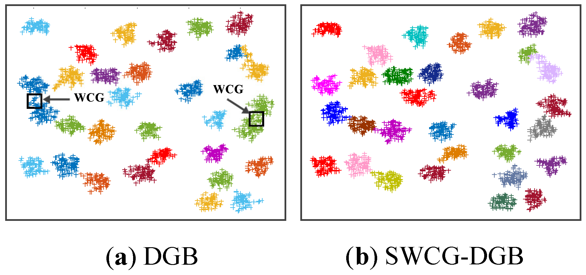
Following the approach and measuring metrics shown in Subsection 4.1 and 4.2, we obtained the results in Figure 6, Figure 7, Figure 8, Figure 9, Figure 10 and Figure 11 and Table 3 and Table 4.

First, we employed the five methods to cluster Dataset 1, which contains 3300 two-dimensional data points with 5% noise and RNC=9 (see Figure 5 and Table 1). The results in Figure 6 and Table 3 reflect that the SWCG-DGB could cluster the database correctly with QNC= RNC=9. The other methods are inferior to the SWCG-DGB. Namely, QNC=3 for the DGB, QNC=8 for the DBSCAN, and QNC=10 for the DPCSA. For the DPC and HDBSCAN, despite the accurate number of clusters (QNC=9=RNC), some confusion between border points and noise is present in imperfect data clusters.

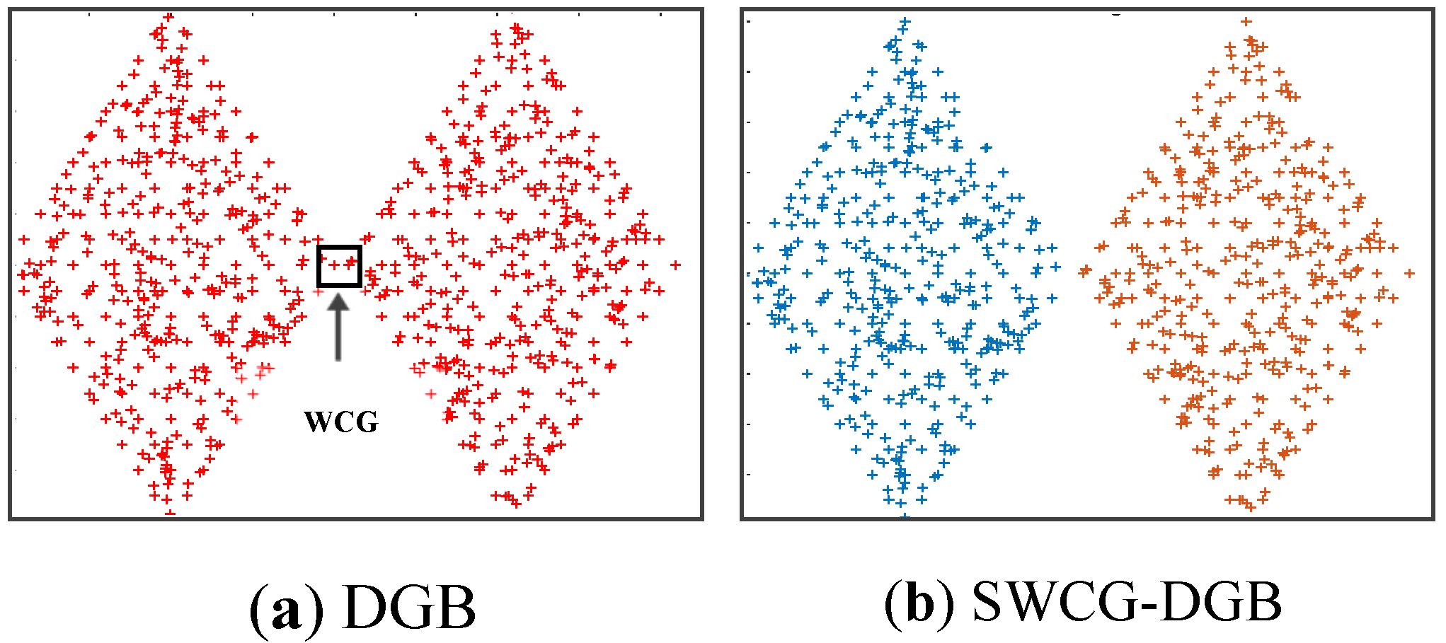
For Dataset 2, Figure 7 and Table 3 show the SWCG-DGB could find the correct number of clusters (QNC= RNC=2), while the DGB is incorrect with QNC=1.

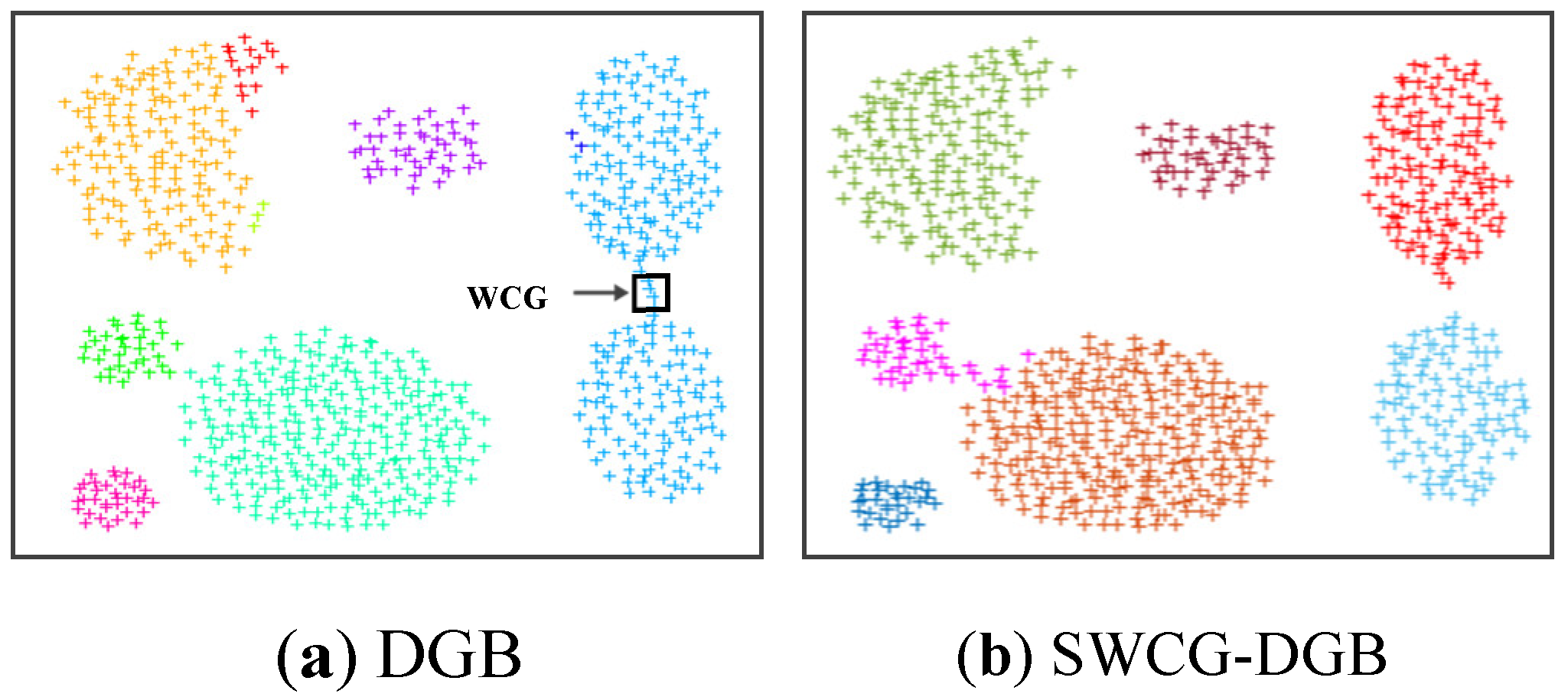
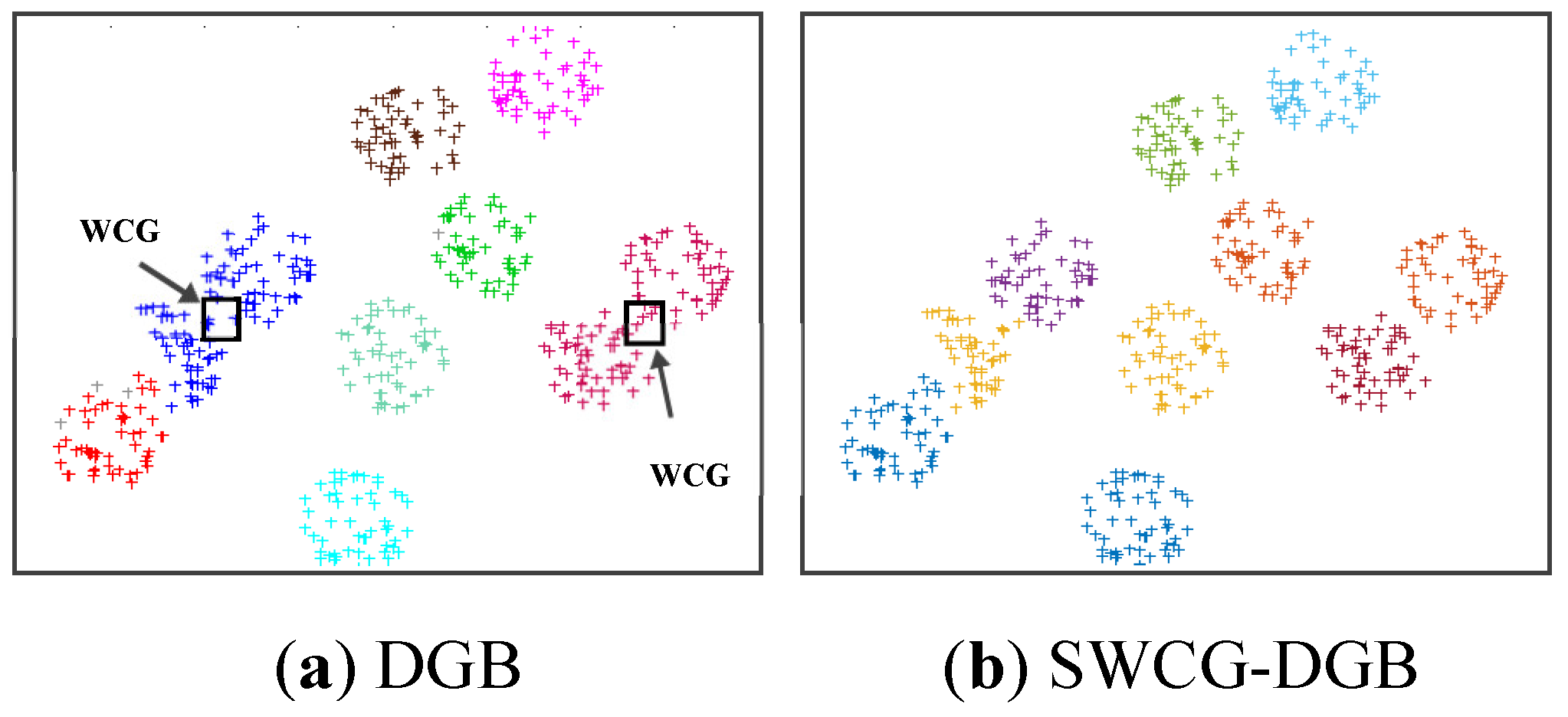
For Dataset 3 and Dataset 4, the compared effectiveness of the SWCG-DGB is much the same. Figure 8 and Figure 9 and Table 3 depict QNC=RNC=7 for Dataset 3 and QNC= RNC=31 for Dataset 4 based on the proposed method.

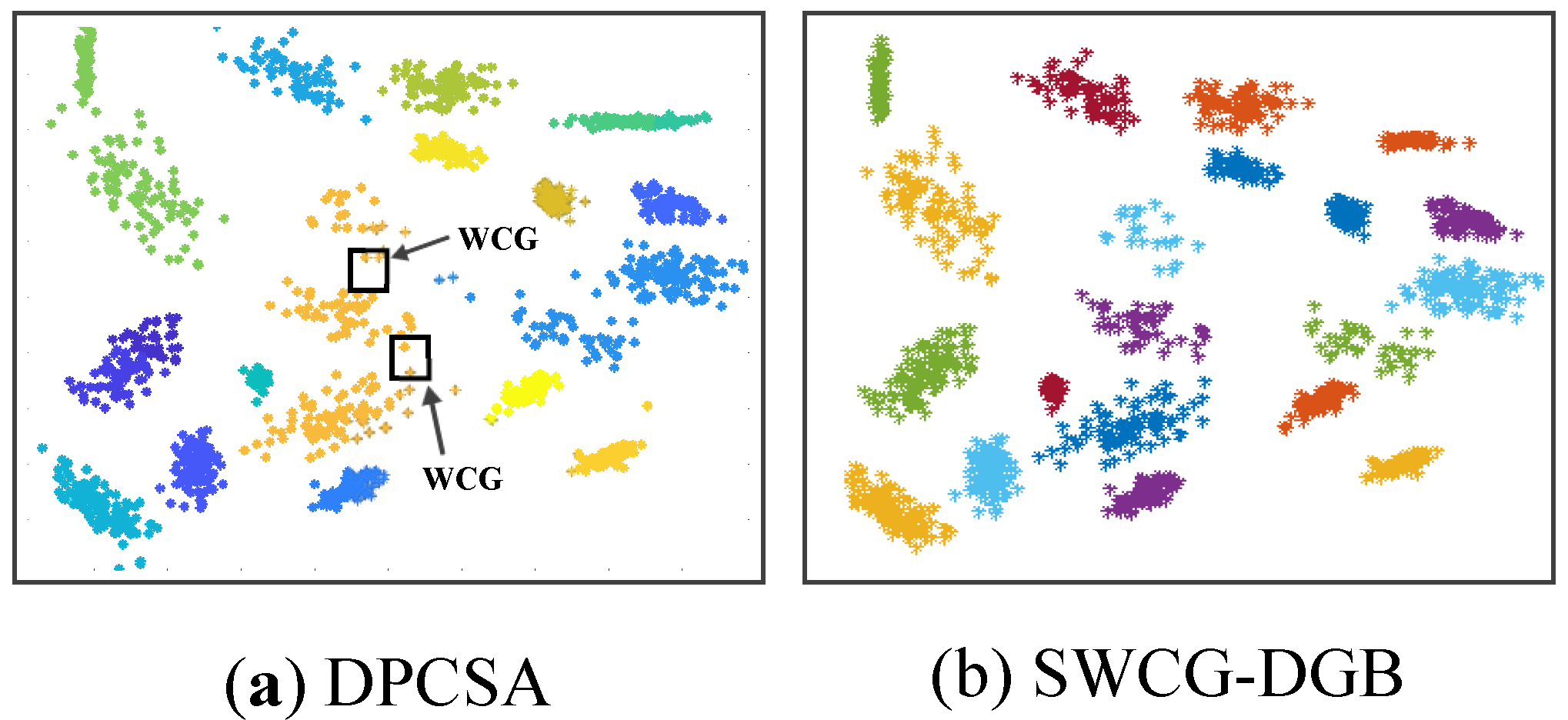
Similarly, for Dataset 5 and Dataset 6 in Figure 10 and Figure 11 and Table 3, they show the accuracy of the SWCG-DGB better than DGB with QNC=RNC=10, and DPCSA with QNC=RNC= 20 regarding Dataset 5 and 6, respectively.

In other words, the SWCG-DGB could always accurately quantify the cluster data space of the datasets in Table 2, even in the presence of noise in the case of Dataset 1. Its advantage is the capability to recognize WCGs to adjust finely and re-establish the created CDS more reasonably. It is easy to see from Figure 6, Figure 7, Figure 8, Figure 9, Figure 10, Figure 11, Figure 12 and Figure 13 that the WCG generated a bridge between two adjacent clusters to form either an inappropriately larger one or data clusters with unsuitable data distribution. This aspect is the main reason for the incorrect results of the method DGB.

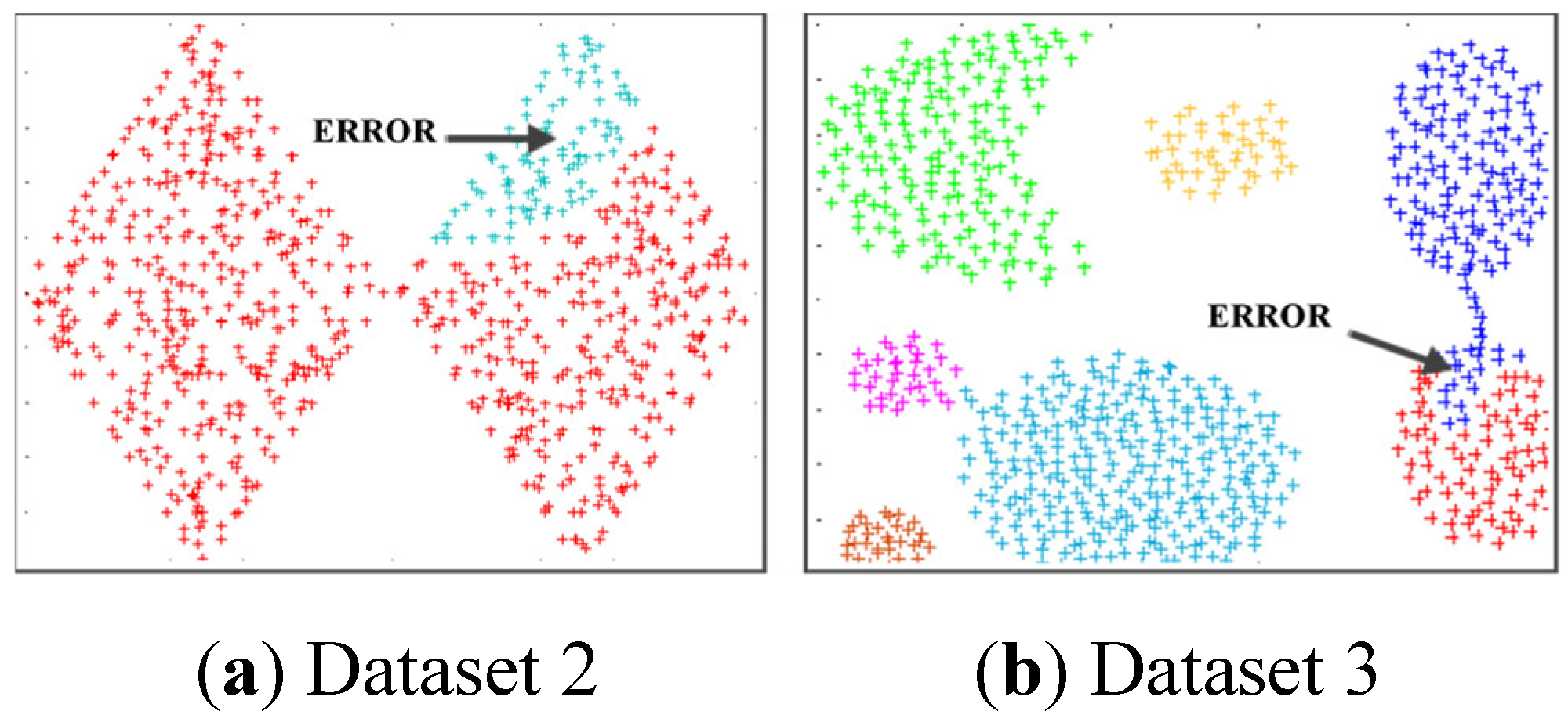
Besides, Figure 12 reflects the incorrect clustering results of the DPCSA when facing Dataset 2 and Dataset 3 as for Dataset 1 of the DPC in Figure 6. In this case, the WCG causes the data classification error denoted in the figure. Similarly, Figure 13 shows that WCG leads to the incorrect QNC of Dataset 3 and Dataset 4 with the HDBSCAN. It is much the same as the issue of the DGB abovementioned. Owning the ability to recognize WCGs, the proposed SWCG-DGB can overcome these difficulties to set up the fit cluster data spaces illustrated in Table 3 and Figure 6, Figure 7, Figure 8, Figure 9, Figure 10 and Figure 11.

Together with evaluating the clustering validity via comparing the QNC and RNC and estimating the reasonableness of data distribution in each cluster, we also surveyed the running time or calculating time (CT) of the methods. Table 3 and Table 4 show that the SWCG-DGB is the best in the clustering validity but is not the fastest method. However, their difference is not much.

In addition, the performance of the clustering is then evaluated using three metrics, including RI, ARI, and NMI. We show the metrics on the six synthetic datasets in Table 1. The results are shown in Table 5, Table 6 and Table 7, and the best results are highlighted in boldface in each column.

Following the results reported, in most instances, the proposed method obtained the best results. From these results, we can see clearly that the performance of the SWCG-DGB is much better than the other clustering methods.

4.3. Simulating Results on Real Datasets

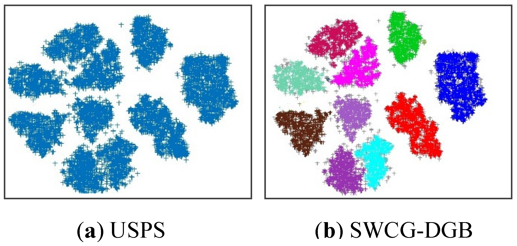
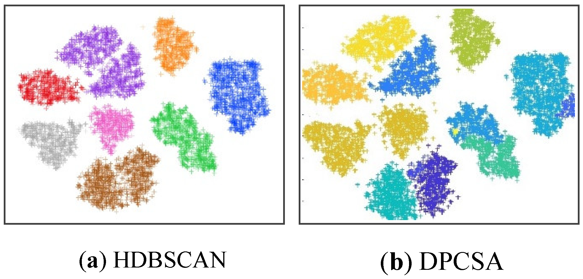
In this section, we compare the capacity of six clustering algorithms on three real datasets that described in Table 1. Namely, Figure 14 and Figure 15 show one popular image data set (USPS) [30], which the U.S. postal service collects from handwritten numbers on envelopes, along with the correctly clustered result of the proposed algorithm and the incorrectly clustered results of the HDBSCAN and DPCSA. All results on the number of clusters are shown in Table 8 below. In general, for all three real datasets, the SWCG-DGB could find the correct number of clusters (QNC= RNC), similar to the DGB, while the remainder methods had some incorrect cases.

Besides, the clustering results obtained in Table 9 evaluate the surveyed methods via the RI, ARI, and NMI using these real datasets. In each column, the best results are highlighted in boldface. It can see that the proposed method yields the best results in most cases.

5. Conclusions

The essential improvement to the density grid-based clustering to propose the method named SWCG-DGB has been presented. This approach has a remarkable advantage related to WCGs in solving the common issue of density grid-based clustering. The task of seeking WCGs to remove noise and adjust the created CDS takes a vital role in improving the clustering validity, including filtering noise and fine-tuning the CDS. In this phase, the calculating strategy without the Euclidean distance is to decrease the complexity of the clustering process. Besides, the buffer explored to store features of data points and coordinates of the grid cells is a fit technique solution. It allows for reducing considerable computational time in filtering noise and updating border points.

Many survey results show that the proposed SWCG-DGB can always better accurately quantify the cluster data space of the given datasets. Accordingly, clustering validity based on the SWCG-DGB is better than the other considered methods. However, the calculating cost is not a comparative advantage of this method. Improving the calculating time, hence, is our motivation in the following research.

Acknowledgments

The authors would like to express their gratitude to the Vietnam National Foundation for Science and Technology Development (NAFOSTED) under grant number 107.01-2019.328.

Conflicts of Interest

The authors declare that we have no conflict of interests or personal relationships that could have appeared to influence the work reported in this paper.

References

Salem; Semeh Ben; Sami Naouali; Zied Chtourou. A fast and effective partitional clustering algorithm for large categorical datasets using a k-means based approach. Computers & Elect. Eng. 2018, 68, 463–483. [Google Scholar] [CrossRef]
Chaira; Tamalika. A novel intuitionistic fuzzy C means clustering algorithm and its application to medical images. Applied soft computing. 2011, 1711–1717. [Google Scholar] [CrossRef]
Saxena; Amit; et al. A review of clustering techniques and developments. Neurocomputing. 2017, 267, 664–681. [Google Scholar] [CrossRef]
Li, S.; Li, L.; Yan, J.; He, H. SDE: A novel clustering framework based on sparsity-density entropy. IEEE Transactions on Knowledge and Data Engineering. 2018, 1575–1587. [Google Scholar] [CrossRef]
Saelens, W.; Cannoodt, R.; Saeys, Y. A comprehensive evaluation of module detection methods for gene expression data. Nature comm. 2018, 1090. [Google Scholar] [CrossRef] [PubMed]
Ester, M.; Kriegel, H. P.; Sander, J.; Xu, X. A density-based algorithm for discovering clusters in large spatial databases with noise. kdd. 1996, 226–231. [Google Scholar]
Cheng; Yizong. Mean shift, mode seeking, and clustering. IEEE transactions on pattern analysis and machine intelligence, 1995; 790–799.
Georgoulas, G.; Konstantaras, A.; Katsifarakis, E.; Stylios, C. D.; Maravelakis, E.; Vachtsevanos, G. J. “Seismic-mass” density-based algorithm for spatio-temporal clustering. Expert Systems with Applications, 2013; 4183–4189. [Google Scholar]
Marques; João C. ; Michael B. Orger. “Clusterdv: a simple density-based clustering method that is robust, general and automatic.” Bioinformatics, 2019, 2125-2132.
Chang; Hong; Dit-Yan Yeung. Robust path-based spectral clustering. Pattern Recognition, 2008; 191–203. [CrossRef]
Chen; Xinquan. A new clustering algorithm based on near neighbor influence. Expert Systems with applications, 2015; 7746–7758. [CrossRef]
Huang; Anna. Similarity measures for text document clustering. Proceedings of the sixth new zealand computer science research student conference (NZCSRSC2008), Christchurch, New Zealand, 2008, 9–56.
Uncu, O.; Gruver, W. A.; Kotak, D. B.; Sabaz, D.; Alibhai, Z.; Ng, C. GRIDBSCAN: GRId density-based spatial clustering of applications with noise. 2006 IEEE Inter. Conf. on Systems, Man and Cybe. vol. 4. IEEE, 2006, 2976-2981.
Chen, Y.; Tang, S.; Bouguila, N.; Wang, C. , Du, J.; Li, H. A fast clustering algorithm based on pruning unnecessary distance computations in DBSCAN for high-dimensional data. Pattern Recog, 2018, 83, 375–387. [Google Scholar] [CrossRef]
Marques; J. C.; Orger, M. B. Clusterdv: a simple density-based clustering method that is robust, general and automatic. Bioinformatics, 2019, 2125-2132. [Google Scholar] [CrossRef]
Campello; R. J.; Moulavi, D.; Sander, J. Density-based clustering based on hierarchical density estimates. Pacific-Asia conf. on knowledge discovery and data mining. Springer, Berlin, Heidelberg, 2013, 160-172.
McInnes, L.; Healy, J.; Astels, S. hdbscan: Hierarchical density based clustering. J. Open Source Softw, 2017; 205. [Google Scholar] [CrossRef]
Rodriguez, A.; Laio, A. Clustering by fast search and find of density peaks. Science, 2014; 1492–1496. [Google Scholar] [CrossRef]
Yu, D.; Liu, G.; Guo, M.; Liu, X.; Yao, S. Density peaks clustering based on weighted local density sequence and nearest neighbor assignment. IEEE Access, 2019; 7, 34301–34317. [Google Scholar] [CrossRef]
Wu; Bo; Bogdan M. Wilamowski. A fast density and grid based clustering method for data with arbitrary shapes and noise. IEEE Transactions on Industrial Informatics, 2016; 1620–1628. [CrossRef]
Cheng, C. H.; Fu, A. W.; Zhang, Y. Entropy-based subspace clustering for mining numerical data. Proceedings of the fifth ACM SIGKDD international conference on Knowledge discovery and data mining, 1999; 84–93. [Google Scholar]
Duan, D.; Li, Y.; Li, R.; Lu, Z. “Incremental K-clique clustering in dynamic social networks. Artificial Intelligence Review, 2012; 129–147. [Google Scholar] [CrossRef]
Chen, Y. , Tu, L. Density-based clustering for real-time stream data. Proceedings of the 13th ACM SIGKDD Inter. Conf. on Knowledge discovery and data mining, 2007, 133-142.
Li, H.; Wu, C.; Jing, X.; Wu, L. Fuzzy tracking control for nonlinear networked systems. IEEE Transactions on Cybernetics, 2016; 2020–2031. [Google Scholar] [CrossRef]
Nguyen; Sy Dzung; Vu Song Thuy Nguyen; Nhat Truong Pham. Determination of The Optimal Number of Clusters: A Fuzzy-set based Method. IEEE Transactions on Fuzzy Systems, 2021. [CrossRef]
Van Der Maaten; Laurens. Accelerating t-SNE using tree-based algorithms. The journal of machine learning research, 2014; 3221–3245.
Rand; William M. Objective criteria for the evaluation of clustering methods. Journal of the American Statistical association, 1971; 846–850.
Hubert, L.; Arabie, P. Comparing partitions journal of classification 2 193–218. Google Scholar, 1985; 128–193. [Google Scholar]
Strehl, A.; Ghosh, J. Cluster ensembles---a knowledge reuse framework for combining multiple partitions. Journal of machine learning research 3. Dec 2002, 583–617. [Google Scholar]
https://www.csie.ntu.edu.tw/cjlin/libsvmtools/datasets/multiclass.html.

Figure 1. Neighbors of cell g in two-dimension data space.

Figure 2. A WCG appearing between the two clusters in the two-dimension data space.

Figure 3. Node’s local density in the two-dimensional data space.

Figure 4. Workflow for searching the WCGs.

Figure 5. The six benchmark datasets: 9Diamonds (Dataset 1), 2Diamonds (Dataset 2), Aggregation (Dataset 3), D31 (Dataset 4), Elliptical (Dataset 5), and 2D-20C (Dataset 6).

Figure 6. The comparative results deriving from Dataset 1 and the six methods consisting of DGB (no_grid=20), SWCG-DGB (no_grid=20), HDBSCAN (minPts=15), DBSCAN (minPts=14; ε=4), DPC, and DPCSA.

Figure 7. The comparative results between the SWCG-DGB and DGB (no_grid=22) with Dataset 2.

Figure 8. The comparative results between the SWCG-DGB and DGB (no_grid=16) with Dataset 3.

Figure 9. The comparative results between SWCG-DGB and DGB (no_grid=55) with Dataset 4.

Figure 10. The comparative results between SWCG-DGB and DGB (no_grid=44) with Dataset 5.

Figure 11. The comparative results between SWCG-DGB (no_grid=44) and DPCSA with Dataset 6.

Figure 12. The incorrect clustering results of the method DPCSA with Dataset 2 and Dataset 3.

Figure 13. The incorrect clustering results of the method HDBSCAN with Dataset 3 and 4.

Figure 14. The original USPS dataset and correctly clustering results of the proposed method SWCG-DGB (no_grid=66) on it.

Figure 15. The incorrect clustering results of the methods HDBSCAN (minPts=15) and DPCSA with the number of clusters in the USPS dataset are 12 and 11, respectively.

Table 1. Details of the datasets.

Datasets	Samples	Dimension	RNC	Noise
Dataset 1 (9Diamonds) Dataset 2 (2Diamonds) Dataset 3 (Aggregation) Dataset 4 (D31) Dataset 5 (Elliptical) Dataset 6 (2D-20C)	3300 800 788 3100 500 1517	2 2 2 2 2 2	9 2 7 31 10 20	Yes (5%) No No No No No
Dataset 7 (Iris) Dataset 8 (Seeds) Dataset 9 (USPS)	150 210 9298	4 7 256	3 3 10	No No No

Table 2. Input parameters of the methods in each survey.

Datasets	HDBSCAN	DBSCAN	DGB	SWCG-DGB
Datasets	minPts	minPts /ε	no_grid	no_grid
Dataset 1 Dataset 2 Dataset 3 Dataset 4 Dataset 5 Dataset 6	15 15 15 15 15 15	4 / 0.12 3 / 0.6 4 / 1.0 10 / 0.6 10 / 0.6 10 / 0.6	20 22 16 55 44 44	20 22 16 55 44 44
Dataset 7 Dataset 8 Dataset 9	15 15 15	6 / 0.16 10 / 0.2 4 / 0.12	60 34 66	60 34 66

Table 3. The number of clusters corresponding to each dataset quantified by the methods (QNC), where the bold values reflect the correct quantified cases (QNC= RNC).

Methods			Datasets
Methods	1	2		3	4	5			6
DBSCAN HDBSCAN DPC DPCSA DGB SWCG-DGB	8 9 9 10 3 9	1 2 2 2 1 2		9 6 7 7 6 7	29 28 31 31 29 31	7 8 10 10 8 10			23 18 19 18 12 20

Table 4. The calculating time (CT) of the algorithms.

Method			Datasets
Method	1	2		3	4	5			6
DBSCAN HDBSCAN DPC DPCSA DGB SWCG-DGB	0.336 0.044 1.215 2.459 0.464 0.356	0.860 0.015 0.621 0.596 0.923 0.513		0.559 0.011 0.372 0.548 0.487 0.361	1.347 0.033 1.952 2.686 1.487 1.457	0.871 0.020 0.413 0.661 0.423 0.302			3.012 0.049 1.114 2.577 0.590 0.352

Table 5. Comparison of results of the algorithms in terms of Rand Index (RI).

Method			Datasets
Method	1	2		3	4	5			6
DBSCAN HDBSCAN DPC DPCSA DGB SWCG-DGB	0.792 0.951 0.954 0.801 0.798 0.972	0.756 0.910 0.918 0.721 0.756 0.942		0.795 0.936 0.970 0.820 0.812 0.976	0.730 0.960 0.976 0.919 0.852 0.961	0.786 0.971 0.972 0.716 0.721 0.983			0.798 0.906 0.922 0.738 0.797 0.936

Table 6. Comparison of results of the algorithms in terms of Adjusted Rand Index (ARI).

Method			Datasets
Method	1	2		3	4	5			6
DBSCAN HDBSCAN DPC DPCSA DGB SWCG-DGB	0.641 0.743 0.891 0.750 0.727 0.904	0.632 0.801 0.910 0.603 0.689 0.915		0.755 0.819 0.922 0.729 0.734 0.939	0.623 0.805 0.908 0.835 0.780 0.942	0.704 0.901 0.855 0.461 0.627 0.913			0.720 0.602 0.896 0.590 0.705 0.901

Table 7. Comparison of results of the algorithms in terms of Normalized Mutual Information (NMI).

Method			Datasets
Method	1	2		3	4	5			6
DBSCAN HDBSCAN DPC DPCSA DGB SWCG-DGB	0.716 0.832 0.841 0.765 0.742 0.932	0.702 0.815 0.816 0.678 0.713 0.928		0.811 0.875 0.972 0.790 0.789 0.953	0.718 0.855 0.953 0.862 0.832 0.957	0.723 0.940 0.912 0.524 0.664 0.952			0.755 0.723 0.811 0.622 0.765 0.933

Table 8. The number of clusters corresponding to each real dataset quantified by the methods (QNC), where the bold values reflect the correct quantified cases (QNC= RNC).

Methods			QNC
Methods		Dataset 7 (Iris)		Dataset 8 (Seeds)			Dataset 9 (USPS)
DBSCAN HDBSCAN DPC DPCSA DGB SWCG-DGB		2 2 3 2 3 3		2 3 3 3 3 3			15 12 9 11 10 10

Table 9. Comparison of results of the algorithms in terms of RI, ARI, and NMI for three real datasets 7-9.

Methods	RI	ARI
Methods	Dataset 7 (Iris)
DBSCAN	0.751	0.682	0.740
HDBSCAN	0.776	0.568	0.733
DPC	0.935	0.893	0.917
DPCSA	0.892	0.886	0.870
DGB	0.955	0.902	0.919
SWCG-DGB	0.962	0.931	0.948
Dataset 8 (Seeds)
DBSCAN	0.782	0.632	0.704
HDBSCAN	0.753	0.413	0.531
DPC	0.921	0.910	0.933
DPCSA	0.746	0.703	0.693
DGB	0.923	0.905	0.910
SWCG-DGB	0.934	0.887	0.895
Dataset 9 (USPS)
DBSCAN	0.675	0.596	0,638
HDBSCAN	0.973	0.868	0.882
DPC	0.927	0.903	0.916
DPCSA	0.851	0.783	0.843
DGB	0.945	0.901	0.916
SWCG-DGB	0.984	0.925	0.938

Disclaimer/Publisher’s Note: The statements, opinions and data contained in all publications are solely those of the individual author(s) and contributor(s) and not of MDPI and/or the editor(s). MDPI and/or the editor(s) disclaim responsibility for any injury to people or property resulting from any ideas, methods, instructions or products referred to in the content.

© 2024 by the authors. Licensee MDPI, Basel, Switzerland. This article is an open access article distributed under the terms and conditions of the Creative Commons Attribution (CC BY) license (http://creativecommons.org/licenses/by/4.0/).

Copyright: This open access article is published under a Creative Commons CC BY 4.0 license, which permit the free download, distribution, and reuse, provided that the author and preprint are cited in any reuse.

MDPI Initiatives

Important Links

Choose an area of interest and we will send you notifications of new preprints at your preferred frequency.

Disclaimer

A Strategy of Weak-Connected Grid Search for Noise Filtering and Density Grid-Based Data Clustering

Abstract

1. Introduction

2. Related Concepts

3. Proposed Method

3.1. Initialization

3.2. Finding the Number of Clusters

3.3. Searching the Weak-Connected Grids

3.4. Filtering Noise and Updating Border Points

4. Experimental Simulation

4.1. Approach

4.2. Evaluation Measures

4.3. Simulating Results on Synthetic Datasets

4.3. Simulating Results on Real Datasets

5. Conclusions

Acknowledgments

Conflicts of Interest

References

MDPI Initiatives

Important Links

Subscribe