Decarbonizing Tall Building Structures: Implementing Machine Learning At The Early-stage Of Design Process

Preprint

Article

Decarbonizing Tall Building Structures: Implementing Machine Learning At The Early-stage Of Design Process

Altmetrics

Downloads

Views

Comments

This version is not peer-reviewed

Submitted:

27 August 2024

Posted:

28 August 2024

You are already at the latest version

Alerts

Abstract

The construction of tall buildings generates a high spatial and temporal concentration of greenhouse gas (GHG) emissions. Research studies have shown that as building height increases, more resources per floor area are required to withstand the increasing effects of lateral loads (wind and earthquake). This has major implications for the environmental performance of tall buildings since the Embodied GHG Emissions (EGHGE) of structural systems tend to represent the greatest portion of the life cycle GHG emissions of tall buildings. This study presents a data driven-based approach for decarbonization of tall buildings and evaluates the significant impact of material types (concrete, steel, and timber), concrete strength, and structural systems relative to a building's height on the EGHGE associated with tall buildings. In mitigating the effects of climate change, this research implements machine learning (ML) algorithms as an early-stage design tool to facilitate the choice of materials, and structural systems for tall buildings. This work considers a wide range of high-rise buildings with four different types of lateral structural systems (Braced-Frame system, Outrigger-Belt system, Shear Wall system, and Tubular system), four different types of construction materials (concrete, steel, hybrid, and timber), varying heights (ranging from 10 to 100 stories), and various concrete materials with different compressive strength ranging from 32 to 90 MPa. Data gathered from more than 100 existing tall building projects along with the data obtained from finite element analysis of 120 high-rise buildings models were utilized to train various ML regression algorithms: Decision Tree, Support Vector Machine, Polynomial Regression, and Elastic-Net Regularized Regression. The performance of ML models was carefully assessed, and the best prediction model was selected to estimate the total amount of CO2 emissions for high-rise buildings. Results indicate that hybrid structures with the Out-Rigger-Belt system exhibit the lowest carbon emission (110 kg/m2) compared to other structural types and systems.

Keywords:

Subject: Engineering - Architecture, Building and Construction

1. Introduction

Resources, such as energy, water, and carbon flow throughout the life cycle of buildings and can be categorized into embodied flows and operational flows. The resources used in building construction and the manufacturing of building materials across their supply chains are known as embodied flows. Initial embodied flows represent the embodied flows of the building as-built, while recurrent embodied flows represent the resources required to produce and replace building materials throughout the period of analysis. Operational flows are resources involved in the operation of buildings which include heating, cooling, ventilation, domestic hot water, lighting, appliances, and cooking. Regulations and current attempts to improve the environmental performance of buildings have principally focused on operational energy(Helal et al., 2019). However, embodied energy can account for a significant portion (up to 60%) of the life cycle energy demand of a building (Hamelin & Zmeureanu, 2014). Additionally, improvements in the operational efficiency of buildings are often achieved using assemblies of high embodied energy such as thermal insulation and advanced façade systems (Fraga-De Cal et al., 2021; Helal et al., 2020). Therefore, as the operational energy efficiency of buildings improves, the operational Greenhouse Gas (GHG) emissions decrease. Over time, a building’s life cycle environmental flows will contain an increasing amount of embodied GHG emissions (EGHGE).

The increasing rate of urbanization has seen an accelerated trend in the construction of tall buildings, intending to increase population density near employment opportunities. In nearly two decades, between 2000 and 2017, there were 1,319 structures higher than 200m, a 400% increase from 263. (Helal et al., 2019). The number and heights of tall buildings are expected to continue growing as a solution to the challenges of urbanization and as a means of establishing compact cities that are attributed to less car dependency, better public transport services, and better health outcomes. However, such construction generates a high spatial and temporal concentration of GHG emissions, a phenomenon such as the ‘carbon spike.’ Tall buildings can have up to 60% more embodied energy per gross floor area than low-rise buildings (Helal et al., 2020). This increase in resource use is mainly due to the cumulative effect of lateral loads on the behavior of tall buildings, whereby more resources per floor area are required for the structural systems of tall buildings to endure the growing influence of seismic and wind stresses. Since most of a tall building’s life cycle GHG emissions are embedded in its structural systems, this has significant effects on the environmental performance of tall structures.

The “premium-for-height” design framework was put up by Bangladeshi-American structural engineer and architect Fazlur Rahman Khan (1967) for the structural systems of tall buildings during the 1960s. Khan argued that the challenge of a structural engineer is to design structural systems that minimize the ‘premium-for-height’ of a tall building as defined by the increase in material per gross floor area with increasing building height (Helal et al., 2018). However, in meeting the challenges of reducing climate change and addressing higher density, minimizing the environmental effects associated with structural systems must become a design priority to achieve high environmental performance in tall buildings.

Machine Learning (ML) methods have shown promising applications in decarbonizing tall buildings. (Giannelos et al., 2023) used ML to forecast CO2 emissions, while (Sanni-Anibire et al., 2021) developed a cost estimation model for tall building projects. (Jiwei Li, 2020) reviewed the use of ML in building energy consumption research, and (Płoszaj-Mazurek, 2020) applied ML to architectural design for carbon footprint reduction. There are also a number of studies investigating the environmental impact of structural elements such as concrete and steel. The predicting ability of ML-based methods in Compressive Strength (CS) and Embodied Carbon (EC) of cement replacement concrete was investigated in (Lavercombe et al., 2021) study. Another approach for mitigating the environmental impact of structural materials is the application of recycled coarse aggregate in concrete (Shang et al., 2022). A crucial component in meeting the CO2 reduction issue is ferrous scrap. Ferrous scrap, on the other hand, is among the most intricate industrial raw resources. Furthermore, scrap has a very diverse range of physical and chemical properties. Certainty on the details of the scrap, however, is necessary to produce high-quality steel products and ML approaches can positively address the environmental challenges for producing high-quality steel (De La Peña et al., 2023).

These studies collectively demonstrate the potential of ML methods in addressing the environmental impact of tall buildings and used materials in various aspects. This research presents an ML-based approach as an early-stage design tool to facilitate the choice of materials, and structural systems for tall buildings. The holistic approach of this study which covers a wide range of structural systems, construction materials, and number of floors could yield reliable outcomes, can be used by decision-makers and stakeholders to estimate the carbon emission of desired buildings in its early-stage.

2. Methodology

The methodology used in this study includes four steps. The first step consists of finite element modeling (FEM) of various tall buildings encompassing four different types of structural systems (shear-wall, out-rigger, brace-frame, and tube), four material types (concrete, steel, timber, hybrid), ten different number of floors for buildings (10, 20, 30, 40, 50, 60, 70, 80, 90, and 100), and finally seven different construction concrete materials covering a wide range of compressive strengths including: 32, 40, 50, 60, 70, 80, 90, 100 MPa. The GHG emissions for each building are determined in the second step. In the third step, a dataset comprising of FEM simulation results along with data from 100 existing tall buildings projects was created and it was used to train various supervised regression ML algorithms such as: Decision Tree, Support Vector Machine, Polynomial Regression, and Elastic-Net Regularized Regression. Finally, in the last step, through comparing the performance of the predictive models, the best ML-based model is selected to estimate the EGHGE. The implemented ML algorithms and their results are discussed in detail in section 4 of this paper.

2.1. Notions and Definitions

2.1.1. Tall Buildings

Among multiple possible definitions, this work adopts the definition for tall buildings proposed by the Council on Tall Buildings and Urban Habitat (CTBUH). As such, this work defines a tall building as a building whose height is at least 35 meters and whose structural design is significantly influenced, because of its height, by lateral forces due to wind or earthquake actions. This adopted definition emphasizes the influence of dynamic lateral loads on tall buildings while underlining the importance of considering them from the beginning of the design process.

2.1.2. Structural Systems

A structural element is a physically distinguishable part of a structure such as a wall, column, beam, slab, or connection. A structural system refers to an arrangement of structural elements capable of resisting loads. Tall buildings are generally composed of two structural sub-systems: a lateral load-resisting system, which predominantly resists wind and earthquake loads; and a vertical load-resisting system, which predominantly resists gravity loads. It is important to note that the actions of these structural sub-systems and their resistance to loading are not mutually exclusive. Due to the complex nature of structural interactions, a vertical load-resisting system moderately resists lateral loads and contributes to the overall lateral stiffness of a tall building and vice versa. This work identifies the following thirteen structural systems for tall buildings: 1) shear wall, 2) braced frame, 3) rigid frame, 4) outrigger and belt, 5) framed tube, 6) braced tube, 7) bundled tube, 8) tube-in-tube, 9) diagrid, 10) space truss, 11) super frame, 12) exoskeleton and 13) buttressed. However, in this research the following four most common important structural systems for tall buildings are considered and studied; 1) shear wall system, 2) braced-frame system, 3) outrigger-belt system, and 4) tube system.

2.2. Data Collection and Determination of Global Warming Potential (GWP)

The dataset was gathered from various sources, including data collection from more than 100 existing high-rise buildings projects along with the data obtained from the FEM analysis of approximately 120 high-rise buildings models encompassing various structural types, lateral systems, and varying numbers of stories. Consequently, CO₂ emissions corresponding to different concrete strengths, including 32, 40, 50, 60, 70, 80, 90, and 100 MPa, were calculated. Major structural elements such as beams, columns, slabs, and core shear wall volume (BOQ) were calculated. This involved calculating the Global Warming Potential (GWP) by multiplying Structural Material Quantities (SMQ) with Embodied Carbon Coefficients (ECC). It should be noted that the accurate determination of ECC values is challenging. The available ECC values, derived from literature, often vary, primarily due to the exclusion of certain life cycle stages such as transportation, construction, and demolition in existing ECCs. However, default ECC values have been defined based on a comprehensive literature review. For instance, unreinforced concrete typically exhibits ECC values between 0.1 and 0.2 kgCO₂e/kg, while reinforced concrete values range from 0.13 to 0.28 kgCO₂e/kg (De Wolf, 2014), contingent upon factors like rebar percentage and material strength. Similarly, steel values exhibit variations depending on multiple factors including location, manufacturing, transportation, fly ash replacement, and recycled content, averaging 0.8 kgCO₂e/kg for hot rolled steel and 1.7 kgCO₂e/kg for rebar.

This research also focuses on case studies, holding material properties and geometric factors constant to isolate the influence of Life Cycle Inventory (LCI) methods on EGHGE. Primary building parameters and their values are selected based on established industry codes of standards, ensuring a comprehensive study of the influence of different factors on EGHGE. Load considerations encompass permanent, facade, wind, and earthquake loads, following the best code of practices in tall building design and construction. Ultimately, the research aims to quantify the embodied greenhouse gas emissions of structural systems in tall buildings by using the following equation-based approach Eq. (1):

{E G H G E}_{S S, L C I} = \sum_{m = 1}^{M} (Q_{m, S S} \times {E G H G E C}_{m, L C I})

where, EGHGE_{SS, LCI} is the amount of embodied GHG emissions of a structural system (SS) in kgCO₂-e calculated using LCI approach (i.e. process-based, input-output-based or hybrid-based). Q _m,ss is the quantity of material “m” in a structural system (SS) (e.g. steel in kg); and EGHGE_cm, LCI is the embodied GHG emissions coefficient of material “m” (e.g. 2.90 kgCO₂-e/kg for hot-rolled steel) developed using life cycle inventory approach LCI. And “M” is a particular component i = 1, 2, 3, ….

3. Finite Element Modeling of Tall Buildings

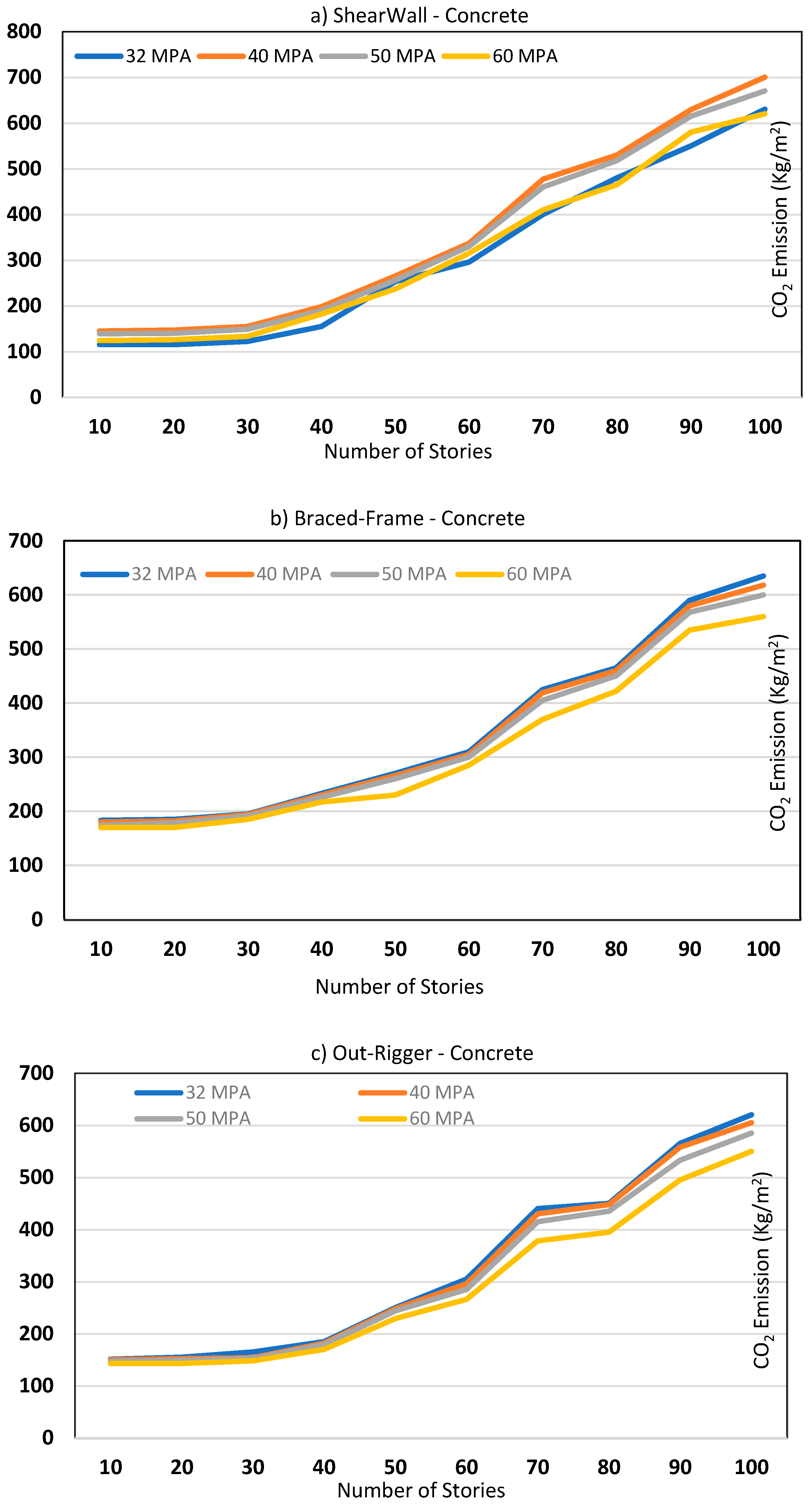
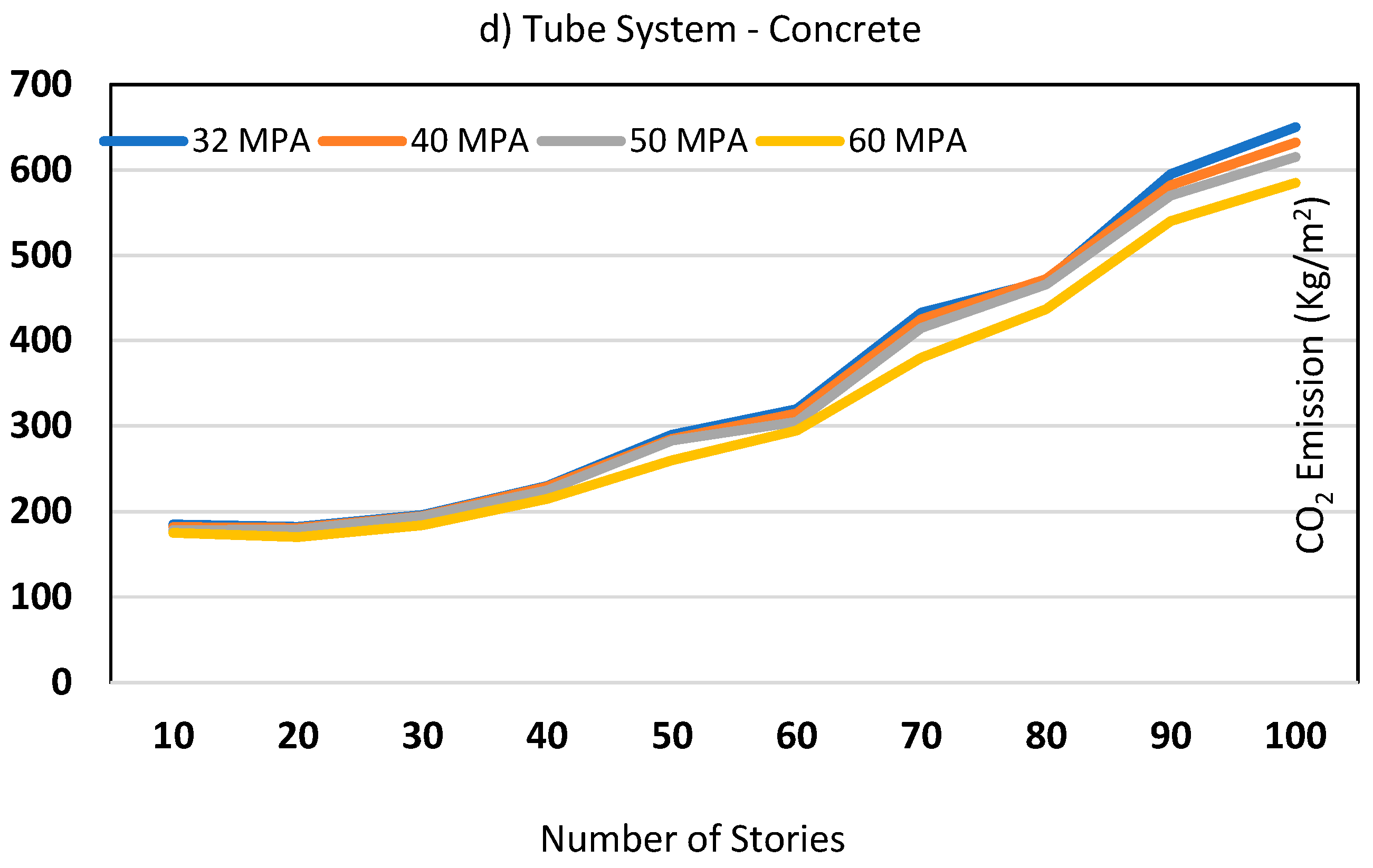
In the present work, finite element analysis of 120 tall buildings was performed using the CSI ETABS software. The FEM simulation of concrete structures revealed that structures with either the shear wall or the out-rigger-belt lateral systems exhibited lower carbon emissions (starting at approximately 150 kg/m²) as compared to braced frame and tube lateral systems, which begin at approximately 180 kg/m². This disparity in emissions can be attributed to the inherent differences in structural behavior and material utilization across these lateral systems. In shear wall and out-rigger-belt systems, the distribution and absorption of lateral forces are primarily facilitated by vertical elements such as walls and belt trusses. These systems are characterized by their relatively higher stiffness and capacity to resist lateral loads, resulting in reduced stresses and deformations throughout the building. Consequently, structural components within these systems can be designed to be smaller and more efficiently proportioned, leading to lower material consumption and, subsequently, reduced CO₂ emissions. On the other hand, braced frame and tube systems often necessitate a more robust and extensive structural framework to withstand lateral forces. The presence of diagonally braced frames or perimeter tube structures requires larger quantities of concrete and steel, contributing to higher initial carbon emissions. Additionally, the increased complexity and redundancy inherent in these systems may lead to higher embodied carbon in construction materials and processes.

Overall, the findings underscore the importance of lateral system selection in mitigating the environmental impact of high-rise concrete structures. By favoring shear wall or out-rigger-belt systems over braced frame or tube systems, designers and engineers can optimize structural performance while minimizing CO₂ emissions. This emphasizes the need for holistic sustainability assessments during the early stages of design, integrating structural analysis, material selection, and environmental considerations to achieve truly sustainable built environments. Figure 1 (a), (b), (c), and (d) are illustrating the CO2 emissions of concrete structures with different structural systems and type of concrete strengths.

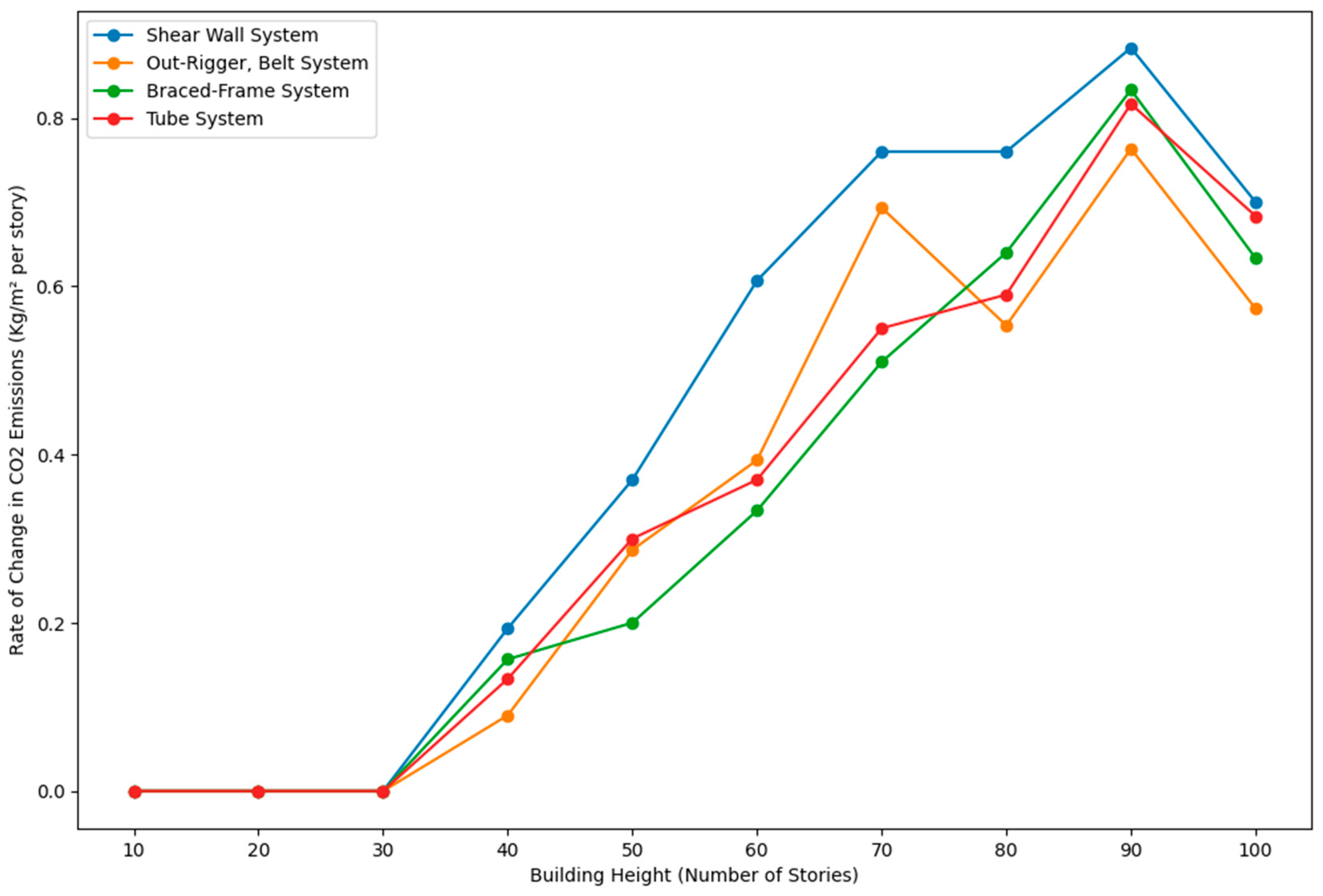
Another interesting observation was the rate of change in CO₂ emissions with respect to height of the building (see Figure 2). Initially, in low-rise buildings with a smaller number of stories, the rate of change in CO₂ emissions tends to be relatively slow. Here, the Shear Wall System, the average rate of change in CO₂ emissions for structures with less than 30 stories is approximately 7.23 kg-CO₂e/m² per story. And for structures with more than 30 stories, this rate increases to approximately 32.28 kg-CO₂e/m² per story. For Out-Rigger, Belt System, the average rate of change in CO₂ emissions for structures with less than 30 stories is approximately 4.17 kg-CO₂e/m² per story. And for structures with more than 30 stories, this rate increases to approximately 27.40 kgCO₂e/m² per story. For Braced-Frame System, the average rate of change in CO₂ emissions for structures with less than 30 stories is approximately 6.63 kg-CO₂e/m² per story. And for structures with more than 30 stories, this rate increases to approximately 25.12 kgCO₂e/m² per story. For Tube System, the average rate of change in CO₂ emissions for structures with less than 30 stories is approximately 5.97 kg-CO₂e/m² per story. And for structures with more than 30 stories, this rate increases to approximately 26.38 kgCO₂e/m² per story.

This can be attributed to several factors. Firstly, the structural demands on low-rise buildings are typically lower, resulting in simpler and more efficient designs with fewer material requirements. Additionally, the embodied carbon emission in these buildings is relatively lower compared to taller structures. As a result, CO₂ emissions associated with the embodied carbon emission remain moderate. However, as buildings exceed a certain threshold, typically around 30 stories or higher, the rate of change in CO₂ emissions begins to increase notably. This acceleration can be attributed to several key factors, notably the structural system design requirements and material selection associated with tall buildings (concrete, steel and hybrid).

In tall buildings, especially those exceeding 30 stories, the lateral forces exerted by wind and seismic loads become significantly stronger. To withstand these forces, structural elements such as columns, beams, and shear walls need to be proportionally larger and stiffer. This results in increased material consumption, particularly of concrete and steel, which are major contributors to CO₂ emissions in construction due to their energy-intensive manufacturing processes. Moreover, the higher portions of tall buildings, where lateral forces are most pronounced, require even greater structural stiffness and strength. This necessitates the use of larger and heavier structural members, further exacerbating the environmental footprint of the building. The relationship between building height and CO₂ emissions is also influenced by the structural system employed. For instance, tall buildings with shear wall system, braced frame, or outrigger-belt system, or tube system exhibit varying levels of materials (concrete, steel, or hybrid) usage and, consequently, differing CO₂ emission profiles. Generally, systems that require more materials (concrete or steel) tend to result in higher emissions.

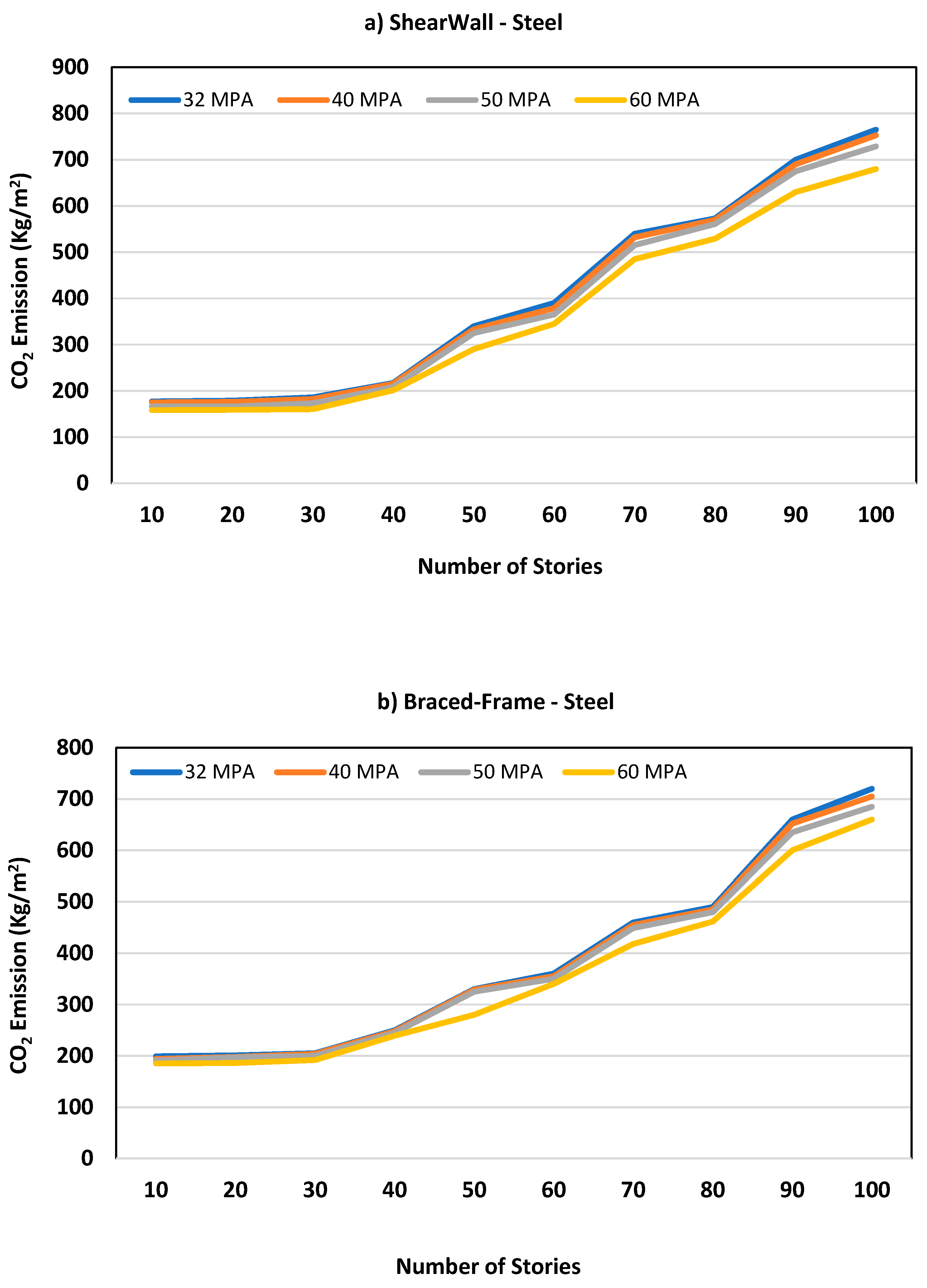
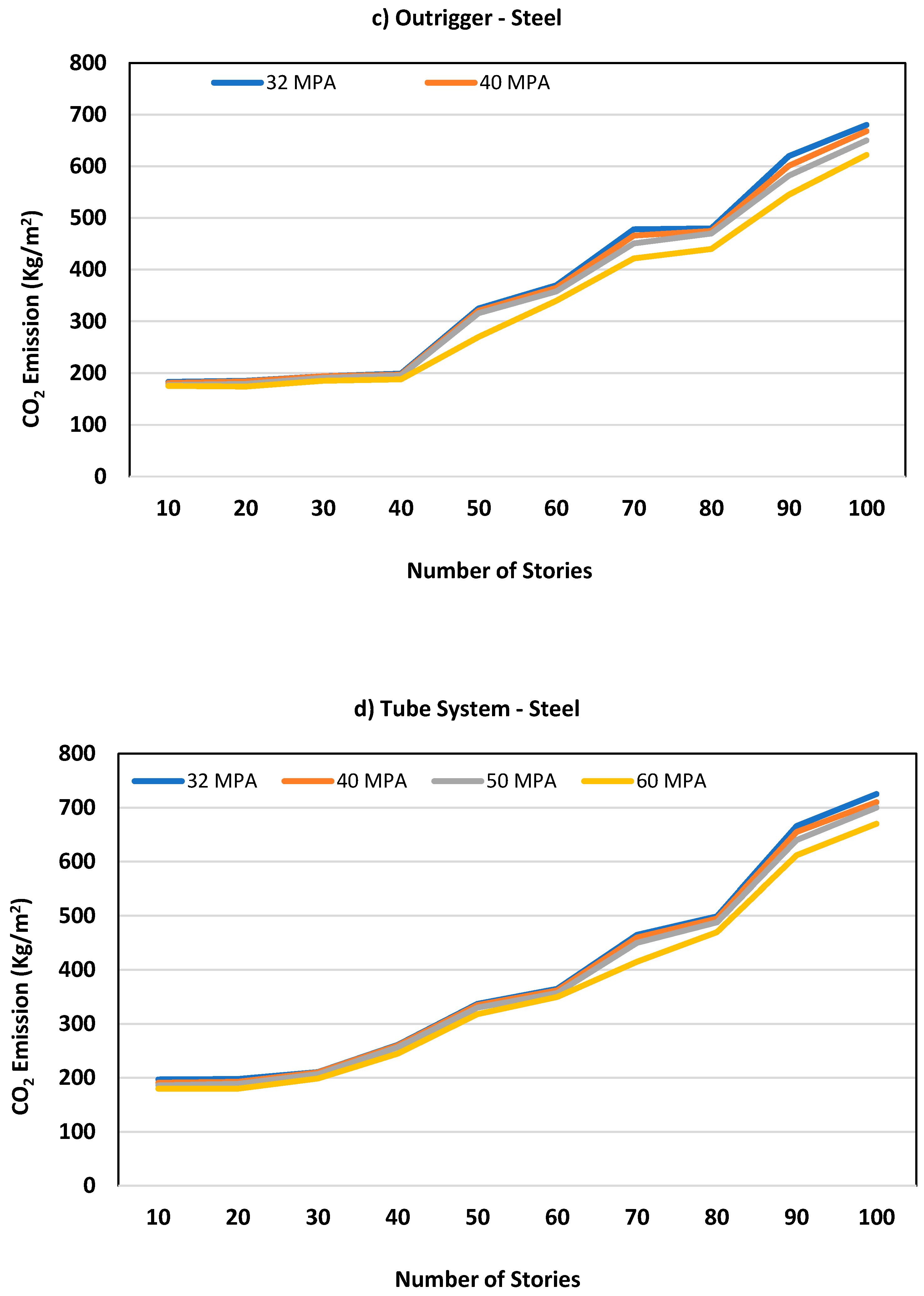
In conclusion, the rate of change in CO₂ emissions with the number of stories in a tall building is initially slow for low-rise structures but accelerates for taller buildings, particularly those exceeding 30 stories. This increase is primarily driven by the heightened structural demands and material requirements (concrete, steel, timber or hybrid) associated with tall buildings, especially in their upper portions where lateral forces are most significant. Understanding these dynamics is crucial for informing sustainable design practices aimed at mitigating the environmental impact of tall buildings. Here, the following graphs, shows analysis of steel structures similar trends and analogy where the structures containing 60 MPa concrete demonstrated the lowest CO₂ emissions across all structural types, starting at approximately 170 kg/m². 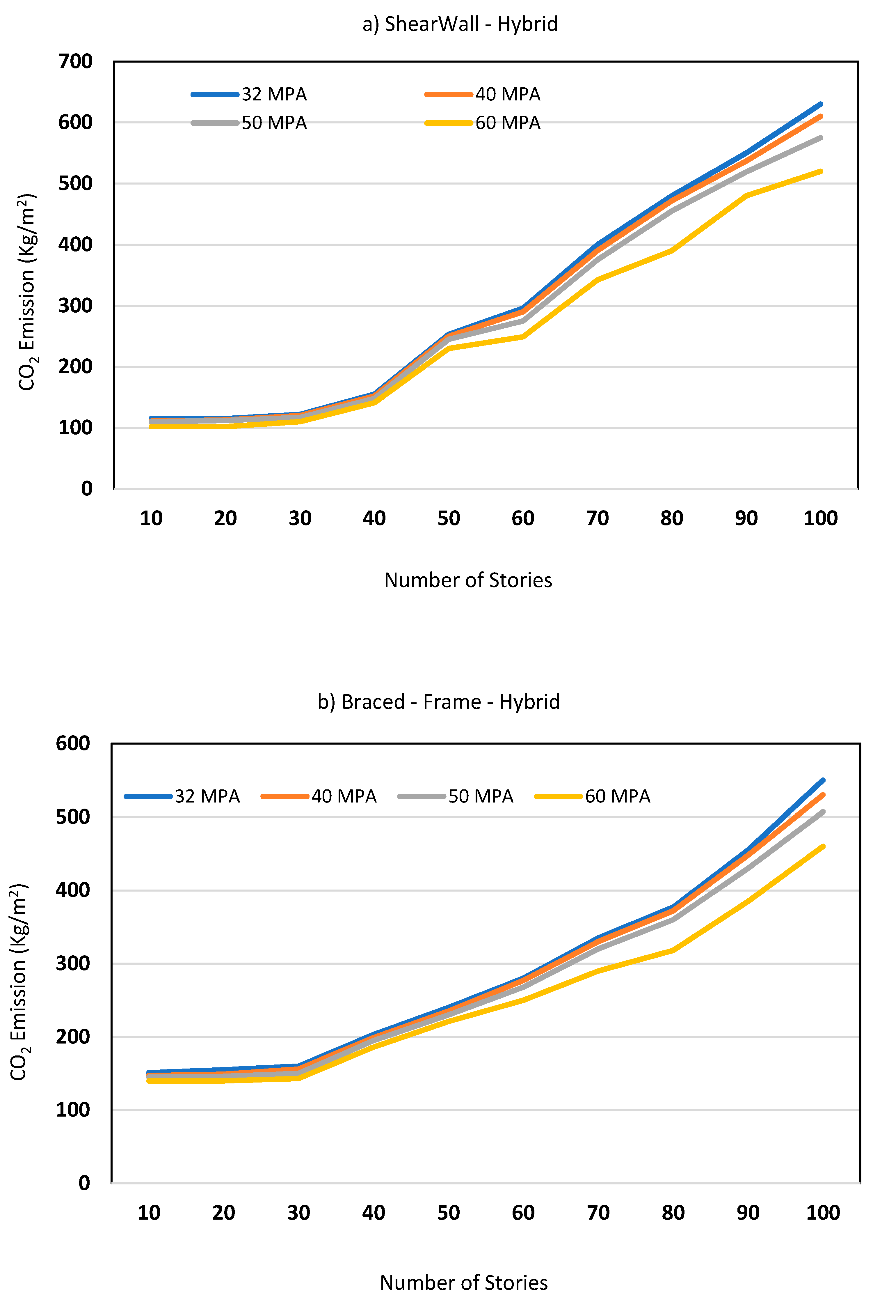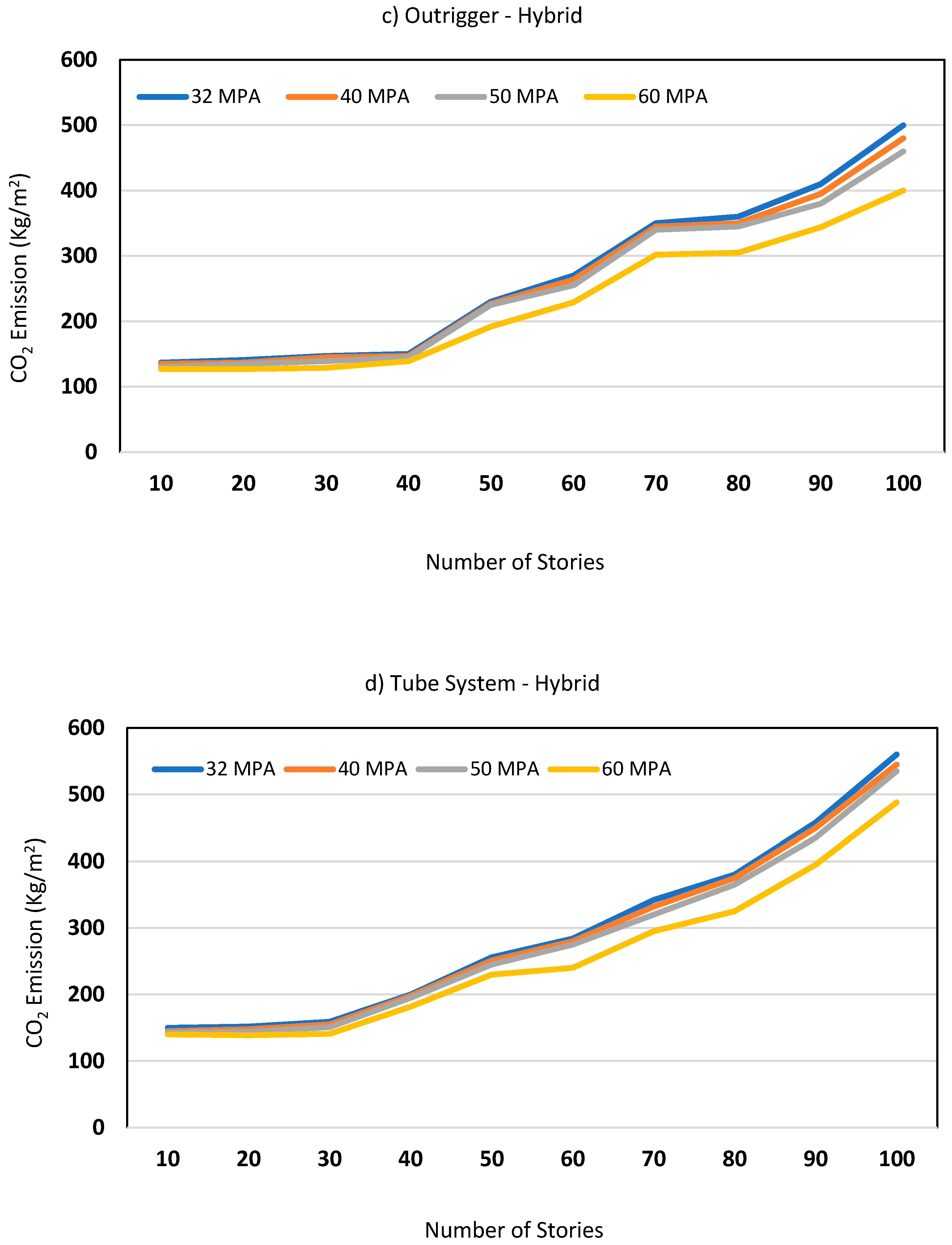Figure 3 (a), (b), (c) and (d) demonstrates this trend in steel structures with Shear Wall Braced Frame, Out-Rigger-Belt, and Tube systems. Moreover, our research findings highlight that hybrid structures demonstrate lower carbon emissions compared to conventional concrete and steel structures in tall buildings above 30 stories.

The same structural system pattern is observed in hybrid structures, with the Out-Rigger-Belt system producing the lowest CO₂ emissions when paired with 60 MPa concrete, starting at approximately 120 kg/m². Figure 4 (a), (b), (c) and (d) showcases the CO₂ emissions of different concrete strengths for a) Out-Rigger-Belts and b) Shear Wall systems. Hybrid structures combine the strengths of different materials, such as concrete, steel and timber, in a synergistic manner. By strategically utilizing each material where it is most efficient, hybrid structures optimize material consumption.

This results in reduced overall embodied carbon compared to traditional concrete or steel structures, where material usage may be less optimized. Hybrid structures often exhibit superior dynamic behavior compared to conventional concrete or steel structures. The combination of different materials can enhance structural resilience and damping characteristics, reducing the need for over-engineering and excess material usage. This dynamic efficiency translates to lower embodied carbon throughout the life cycle of the structure.

In summary, hybrid structures leverage the advantages of multiple materials to achieve lower carbon emissions compared to conventional concrete and steel structures. Through efficient material usage, and using timber, adaptability, dynamic structural behavior, and innovative design approaches, hybrid structures represent a promising pathway towards sustainable construction practices.

Notably, timber structures exhibit the lowest embodied carbon among those structural types at the same category height, with a starting point of 52 kg/m² for 60 MPa concrete. However, it’s important to consider that at this study we analyzed timber structures for projects with a maximum of 20 stories (low to mid-rise buildings). In Table (1), the calculated CO₂ emissions for different timber structures across various concrete types. The results indicate that the Shear Wall structural system, combined with 60 MPa and 70 MPa concrete types, yields the lowest carbon emissions when compared to other structural systems.

Table 1. CO₂ emissions of tall timber structures with different lateral systems for different concrete strength.

		CO₂ Emission
	Concrete Strength (MPa)
Timber Structural Type	No. of Stories	32	40	50	60	70
Shear Wall System	10	62	59	55	52	52
Shear Wall System	20	67	64	63	60	60
Out-Rigger, Belt System	10	75	72	63	57	57
Out-Rigger, Belt System	20	77	75	73	67	59
Braced-Frame System	10	75	71	65	62	62
Braced-Frame System	20	77	74	72	65	58
Tube System	10	73	70	67	65	65
Tube System	20	76	75	72	65	58

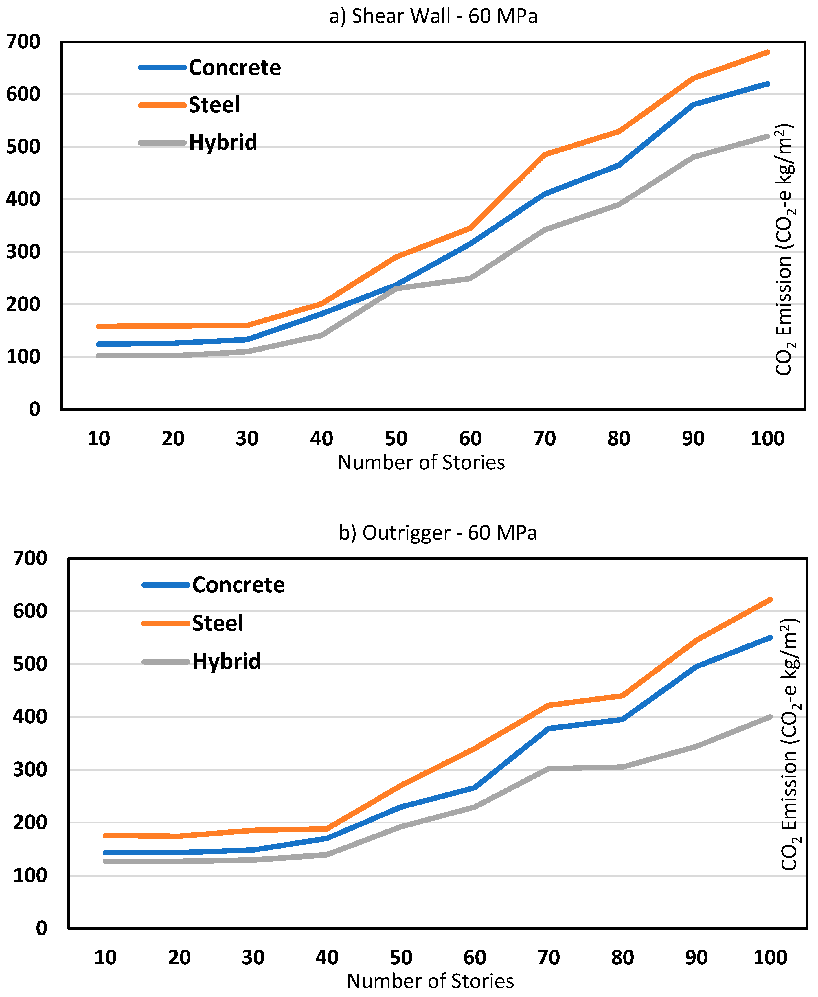
Overall, the relationship between the number of stories in a tall building and its corresponding CO2 emissions is a complex one, influenced by various materials and design factors. As the number of stories increases, we typically observe a trend where CO2 emissions initially rise gradually, reaching a point where the rate of increase accelerates significantly. This phenomenon suggests a non-linear relationship between building height and CO2 emissions. In the subsequent section of this part, results are focused on three structural types: concrete, steel, and hybrid structures, all employing a concrete material with a strength of 60 MPa. The purpose is to visually illustrate which structural type exhibits optimized carbon emissions at each level of tall buildings.

As illustrated below in Figure 5 (a) and (b), hybrid structures consistently demonstrate the most favorable CO₂ emission patterns across various story levels and lateral systems. While the Shear Wall structural system exhibits lower carbon emissions in low to mid-rise structures, the Out-Rigger-Belt structural system outperforms in terms of CO₂ emissions for hybrid structures with 70 or more stories.

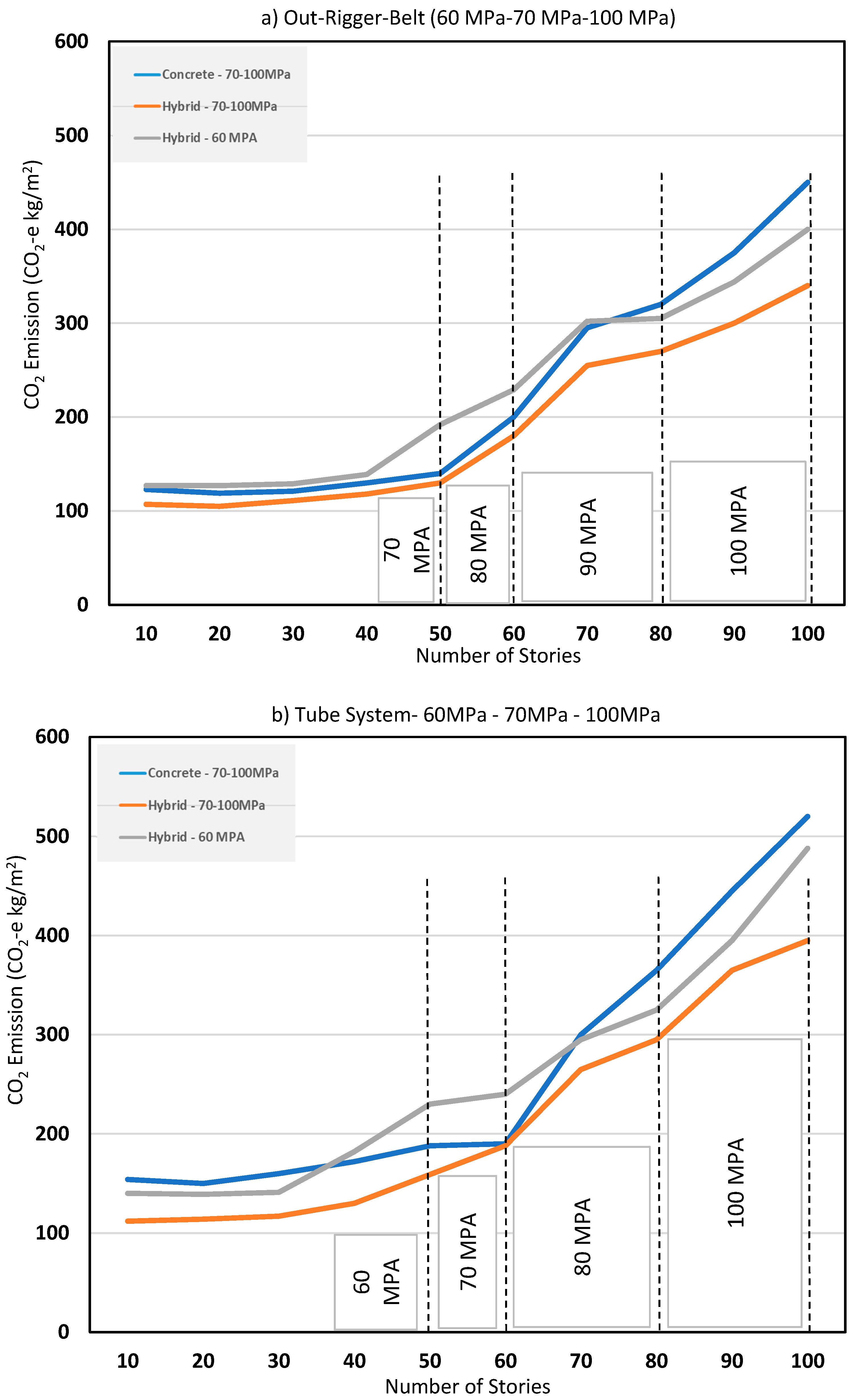
In the subsequent charts, this study compares the CO2 emissions of three different structural types and materials in two lateral systems: the Out-Rigger-Belt system and the Tube system. The aim is to identify the most optimized structural characteristics concerning carbon emissions.

As previously mentioned, hybrid structures with 60 MPa concrete material exhibit the lowest carbon emissions compared to other types, except for timber structures, which are limited to buildings of fewer than 20 stories. To further evaluate hybrid structures, we compare those with 60MPa and 70-100MPa concrete strength in Figure 6 (a) and (b). Given that this study lacks FEM analysis results for carbon emissions with 70-100MPa concrete in these structures across all story levels, and to provide a compact visualization of these concrete types in the structures and their corresponding CO₂ emissions, authors divided the plots with dotted lines. These lines represent the use of 70-100MPa concretes with varying strengths at each story level. For example, at the 50-story level, results for structures with 70 MPa concrete is illustrated, and at 60-story buildings, results for structures with 80 MPa concrete, and so forth.

The results demonstrate that employing higher concrete strength (more than 60MPa) results in lower carbon emissions in structures, irrespective of their lateral systems. Notably, hybrid structures utilizing 60+ MPa concrete consistently exhibit the lowest CO₂ emissions among various structural types. This is particularly pronounced when coupled with the Out-Rigger-Belt structural system.

4. Implementation of Machine Learning Methods

In this research, machine learning algorithms were employed to develop models for prediction of CO₂ emissions. Table (2) below presents the structural features used as input variables for training and testing of ML models. The input features include: 1) number of stories (varies from 10 to 100 stories), 2) lateral system (braced-frame system, out-rigger-belt system, shear wall system, tube system), 3) structural type (concrete, steel, hybrid, and timber structures), and 4) strength of the concrete used in construction of the building (32, 40, 50, 60, 70, 80, 90, 100 MPa).

Table 2. Input features used for developing ML models.

Structural Feature	Value(s)
Number of Stories	10, 20, 30, 40, 50, 60, 70, 80, 90, 100
Lateral System	Braced-Frame System, Out-Rigger-Belt System, Shear Wall System, Tube System
Material Type	Concrete, Steel, Hybrid, Timber
Concrete Strength (MPa)	32, 40, 50, 60, 70, 80, 90, 100

Prior to training ML models, preprocessing of data was performed. This step plays an important role in preparing data for further algorithm implementation, owing to the diversity of data types and scales. Data preprocessing includes handling and manipulating the data to prepare the dataset for use in different algorithms. In the preprocessing stage, the ‘One-hot Encoding’ technique was applied to categorical variables in the dataset, encoding them into numerical variables. Handling noise, outliers, scaling, and missing data are essential steps in the preprocessing stage. However, in this particular dataset, there were no instances of noise, outliers, or missing data that required handling. As a result, categorical values in the dataset, such as the lateral system and the structural systems were encoded into numerical values, respectively. Additionally, the number of stories and the target variable (EGHGE), were normalized. Furthermore, normalization and standardization of the input data was performed to improve the performance of the models. Normalization and standardization are two common techniques used to preprocess data in ML methods. Normalization scales the data to a specific range, often between 0 and 1, while standardization transforms the data to have a mean of 0 and a standard deviation (std) of 1.

In this study, normalization was applied to Decision Tree (DT) and Support Vector Regression (SVR) algorithms, while standardization was used for the Polynomial Regression (PR), and Elastic-Net Regularized Regression. Finally, the dataset was divided into train and test subsets with a ratio of 70% for training and 30% for testing. This separation of the dataset yielded two distinct subsets, with the larger subset used for training algorithms, and the other portion employed to test the models with real, unseen data. The performance of ML models was assessed and compared against each other, and the best performing algorithm was selected. Some of these models contain hyperparameters which require tuning in order to achieve the most optimized predictive models. Thus, the GridSearch approach was utilized to tune the key hyperparameters of ML models. This technique helps to find the best vital hyperparameters for each model to have an optimized predictive model with the highest accuracy. The ML algorithms are briefly introduced in this section.

4.1. Elastic-Net Regularized Regression Method

Elastic-Net is a linear regression model that combines the penalties of Ridge and Lasso regularization to balance their strengths and weaknesses. It adds a linear combination of the L1 (Lasso) and L2 (Ridge) penalty terms to the linear regression loss function. A compromise between Lasso Regression and Ridge Regression is Elastic Net. Elastic Net is comparable to Lasso Regression when r = 1, and to Ridge Regression when r = 0. The Elastic Net is a regularization technique that combines elements from both ridge regression (which uses an L2 penalty) and lasso regression (which uses an L1 penalty). It strikes a balance between the two, allowing you to benefit from both types of regularization. Shrinking the regression coefficient helps prevent overfitting by reducing the complexity of the model and minimizing the impact of individual features on the target variable. Elastic-Net’s Cost function can be defined as Eq. (2).

J (θ) = M S E (θ) + r α \sum_{i = 1}^{n} |θ_{i}| + \frac{1 - r}{2} α \sum_{i}^{n} θ_{i}^{2}

The linear regression objective function aims to minimize the sum of squared differences between the predicted values and the actual target values. It is given by Eq. (3):

J (w, b) = \frac{1}{2 m} \sum_{i = 1}^{m} (y_{i} - (w^{T} x_{i} + b))^{2}

(3)

where:

m : Number of data points.

w : Weight vector (coefficients) for the features.

xi : Feature vector for the ith data point.

b : Bias term.

To prevent overfitting, the Elastic-Net adds regularization terms to the objective function. It combines both L1 (lasso) and L2 (ridge) penalties. The Elastic-Net cost function is given by Eq. (4):

{J (w, b)}_{E l a s t i c N e t} = J (w, b) + α (\frac{1}{2} . (1 - ρ) \sum_{j = 1}^{p} w_{j}^{2} + ρ \sum_{j = 1}^{p} |w_{j}|)

(4)

4.2. Polynomial Regression (PR) Method

PR is an algorithm that models the relationship between input and output variables as an nth degree polynomial. It can capture nonlinear relationships between variables that cannot be adequately represented using linear regression. The calculations involved in PR are similar to those in Linear Regression, but they require transforming input data into higher degree polynomials before fitting a linear regression model. The Eq. (5), defines the general equation for Polynomial Regression can be written as:

y = θ_{0} + θ_{1} x + θ_{2} x^{2} + . . . + θ_{n} x^{n}

(5)

where y is the dependent (target) variable, x is the independent variable, and θ0, θ1, …, θn are the coefficients of the polynomial. The calculations involved in the PR are similar to those in Linear Regression, except that we need to transform our input data into higher degree polynomials before fitting a linear regression model on it. PR is a valuable algorithm for modeling non-linear relationships between input and output variables. Linear regression may not effectively capture these non-linear associations, and PR offers a solution by allowing data to be transformed into higher-degree polynomials. This flexibility made PR a suitable choice for accommodating complex, non-linear patterns and relationships within the data, which is often encountered in real-world scenarios.

4.3. Decision Tree Regression Method

The decision tree for Regression algorithms is a non-parametric supervised learning method employed for regression tasks. It aims to build a model that predicts the value of a target variable by learning simple decision rules derived from the data’s features. A decision tree can be seen as a piecewise constant approximation. The decision trees are easy to understand and interpret, making them suitable for explaining the factors contributing to the predictions. They are versatile and can handle both regression and classification tasks, making them a valuable tool for various types of data analysis. The mathematics behind decision tree regression is relatively easy to understand compared to other machine learning algorithms.

The algorithm works by recursively partitioning the data into subsets based on the values of the input features. The partitioning is done in such a way that it maximizes the homogeneity of the target variable within each subset. This process is repeated until a stopping criterion is met, such as reaching a maximum depth or minimum number of samples per leaf node. Given training vectors , i = 1, …, i and a label vector , a decision tree recursively partitions the feature space such that the samples with the same labels or similar target values are grouped together.

4.4. Support Vector Regression (SVR) Method

The SVR seeks to find a function that approximates the relationship between input variables and a continuous target variable while minimizing prediction error. Mathematically, SVR entails identifying a hyperplane in a high-dimensional space that optimally separates data points into two classes, with the hyperplane being defined by a subset of training data referred to as support vectors. The algorithm operates by mapping input data into a higher-dimensional feature space using a kernel function, enabling the modeling of non-linear relationships. The hyperplane is then found in this feature space, and the predicted output is obtained by projecting it back into the original input space. Additionally, the kernel functions and the importance of support vectors in SVR calculations are explained below. The most commonly used kernel functions include linear, polynomial, radial basis function (RBF), and sigmoid. Eq. (6) demonstrates the Kernel Function equation:

K_{X i, x j} = ϕ_{x i}^{T} ϕ_{x j}

(6)

Support vectors are the data points that lie closest to the decision boundary between different classes and play a pivotal role in shaping the decision boundary. Margin is the distance between the decision boundary and the closest support vectors. The goal of SVR is to find a decision boundary that maximizes the margin while minimizing the prediction error. The calculation of the margin is presented in Eq. (7).

y (x) = θ^{T} ϕ (x) + β

(7)

where y(x) is the predicted output value for input vector x, w is the weight vector that defines the hyperplane in the feature space, ϕ(x) is the feature vector that maps the input vector x into a higher-dimensional space, and β is the bias term that shifts the hyperplane away from the origin.

4.5. Performance Evaluation of ML Models

Statistical metrics such as MAE (Mean Absolute Error), MSE (Mean Squared Error), and R-squared (R2) were employed to evaluate the effectiveness of developed machine learning models. The R2 metric was ultimately selected as the determining metric in identifying the ML model that yields the highest level of performance. The formula for calculating R-squared is presented in Eq. (8):

R^{2} = \frac{\sum_{i = 1}^{n} (\hat{y_{i}} - \overset{ˉ}{y})^{2}}{\sum_{i = 1}^{n} (y_{i} - \overset{ˉ}{y})^{2}}

(8)

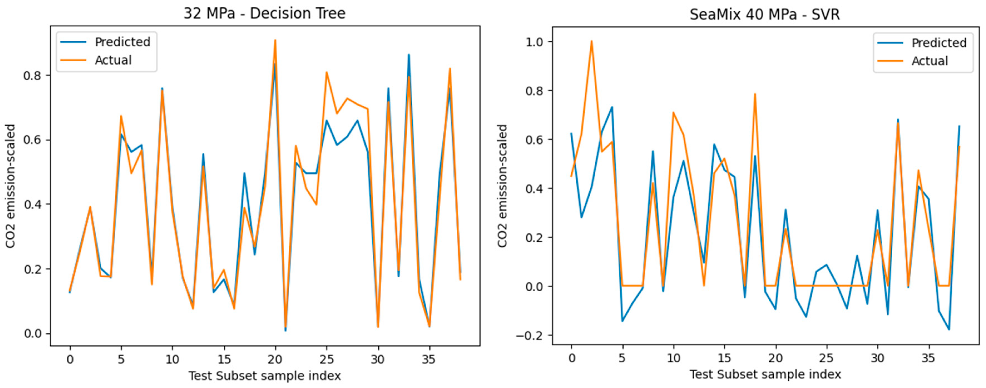
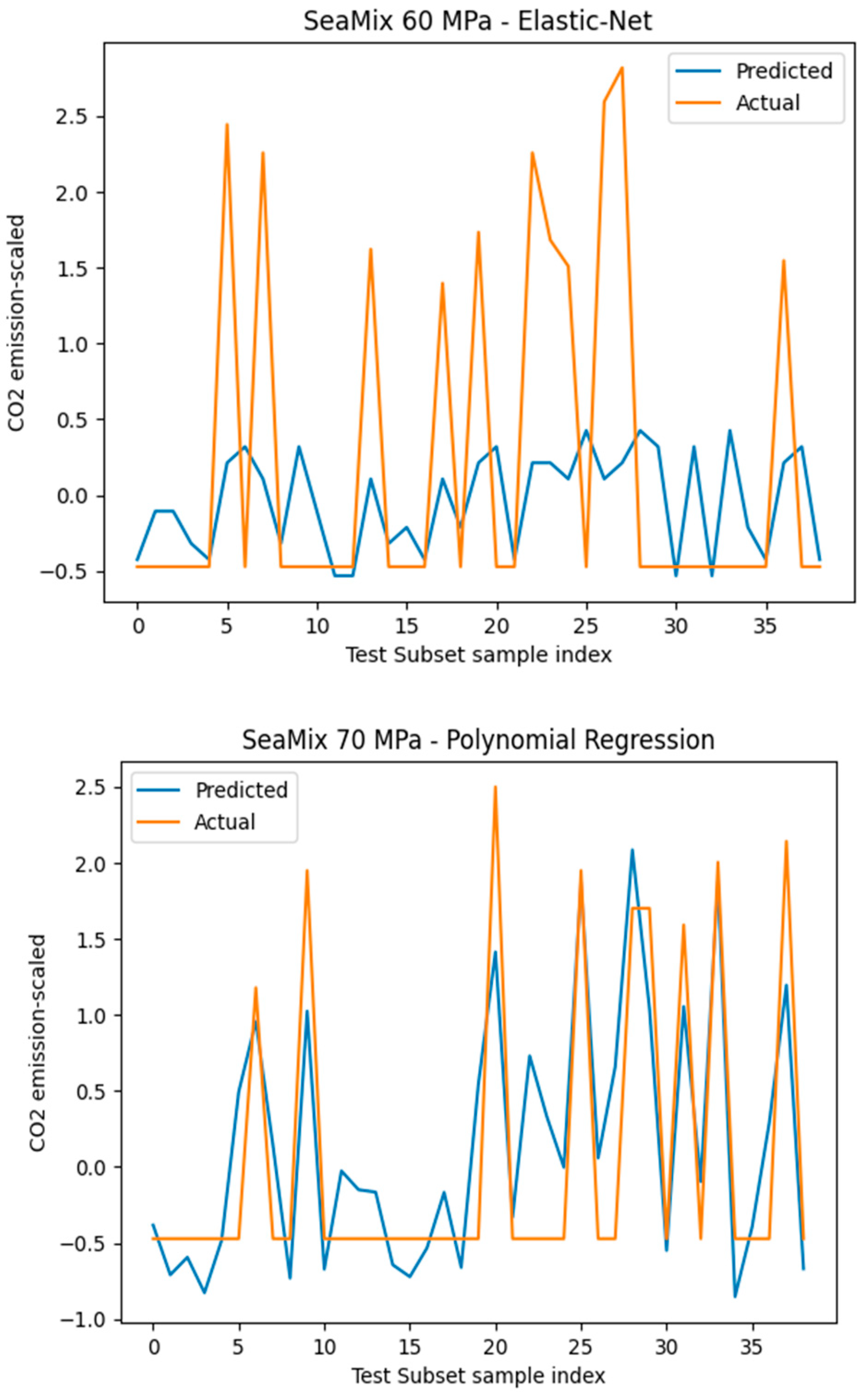
where, is the predicted value of the dependent variable, is the mean value of the dependent variable, is the actual value of the dependent variable, and n is the number of observations. Table (3) presents the R² scores along with the MAE and MSE values of the employed ML models to predict CO₂ emission. The results indicate that the DT algorithm outperformed the other methods with the R² score of 0.99, with the SVR algorithm following closely behind, in comparison to the PR. Given the existence of multiple models, this study presents the predicted against actual values plots, showcasing the predictive capacity of these models in Figure 5 where the horizontal axis represents the index of each sample in the test subset. The dataset was split into training and test subsets with a 70% - 30% ratio, resulting in each test subset containing 308 out of the 1024 available samples. The vertical axis displays the carbon emissions, reflecting the predicted (blue) and actual (orange) CO₂ emission for each model. Results suggest that the practicality of using DT algorithm in predicting CO₂ emission in such dataset consisting of categorical data and numerical data. The Decision Tree (DT) model exhibited exceptional performance with a high R-Squared value of 0.99, indicating a strong fit to the data. However, such a high R-Squared value may suggest overfitting, necessitating caution during model deployment. The DT model also demonstrated the lowest MAE (13) and MSE (452) among the models tested, signifying accurate predictions. In contrast, the Elastic-Net Regression model, designed to mitigate overfitting, achieved the lowest R-Squared (0.63) and highest MAE (100) and MSE (16049) values. While the Elastic-Net model may generalize better to unseen data compared to DT, its predictive accuracy is relatively lower.

Table 3. Comparison of performance of implemented ML models.

ML Model	R2	MAE	MSE
Decision Tree	0.99	13	452
Polynomial Regression	0.81	62	8149
SVR	0.73	68	11746
Elastic-Net	0.68	89	11949

Despite achieving high evaluation scores (high R²), the issue of overfitting remains a concern. The preprocessing step, which includes normalization and transforming categorical values into numerical ones, helps mitigate the risk of overfitting. authors anticipated this challenge due to the impact of the dataset’s sample size (number of rows) on ML-based methods. Nevertheless, authors opted for the ML approach to address innovative objectives within the context of CO₂ emissions.

Figure 7. Performance of predicting values against actual values of ML.

4.6. ML-Based CO2 Prediction Model

The closed-form ML-based model to predict the CO2 emission of tall buildings is presented in Eq. (9).

E = 330.71 + 3.04 L + 3.21 N + 9.45 M_{1} + 35.80 M_{2} - 25.34 M_{3} - 19.91 M_{4} - 4.94 S

(9)

where:

E: The total amount of CO₂ emission in, kgCO₂e/m²

L: Type of “Lateral System” of the building. The following values should be used in the model depending on the type of the lateral system:

L=1 for Braced-Frame System,

L=2 for Out-Rigger-Belt System,

L=3 for Shear Wall System,

L=4 for Tube System

N: Number of stories

M1 - M4: The Material Type and the following values should be used in the model:

Concrete (M1=1, M2=0, M3=0, M4=0)

Steel (M1=0, M2=1, M3=0, M4=0)

Hybrid (M1=0, M2=0, M3=1, M4=0)

Timber (M1=0, M2=0, M3=0, M4=1)

S: Concrete strength in MPa.

This predictive model allows for the assessment of the environmental impact of various structural designs and material choices, aiding in the decision-making process for sustainable construction practices.

4.7. Pearson Correlation Method

The Pearson correlation method, also known as bivariate correlation, was employed for feature selection analysis aimed at reducing the number of input parameters (features) and retaining only the most influential ones for inclusion in the prediction model. This approach effectively reduced training time and mitigated potential overfitting issues. This method quantifies the linear relationship between two variables by calculating the covariance of the variables divided by the product of their standard deviations. In essence, it computes the normalized covariance between two input variables, thereby measuring the linear dependency between two continuous variables. The Pearson product-moment correlation coefficient (a.k.a Pearson’s r) values range from -1 to +1. Given paired data {(

x_{1}

y_{1}

), .… , (

x_{n}

y_{n}

)} consisting of n pairs, the formula for Pearson correlation coefficient (

r_{x, y}

) is expressed as follows:

r_{x, y} = \frac{\sum_{i = 1}^{n} (x_{i} - x ̅) (y_{i} - y ̅)}{\sqrt{\sum_{i = 1}^{n} {(x_{i} - x ̅)}^{2}} \sqrt{\sum_{i = 1}^{n} {(y_{i} - y ̅)}^{2}}} = \frac{σ_{x y}}{σ_{x} σ_{y}}

where n is the sample size (number of datapoints), x_i and y_i are individual sample observations (i.e. measured values of variables),

x ̅

and

y ̅

are the means of x_i and y_i samples, respectively.

σ_{x y}

is the covariance between the features (variables) x and y.

σ_{x}

and

σ_{y}

are the standard deviation of x_i and y_i samples, respectively.

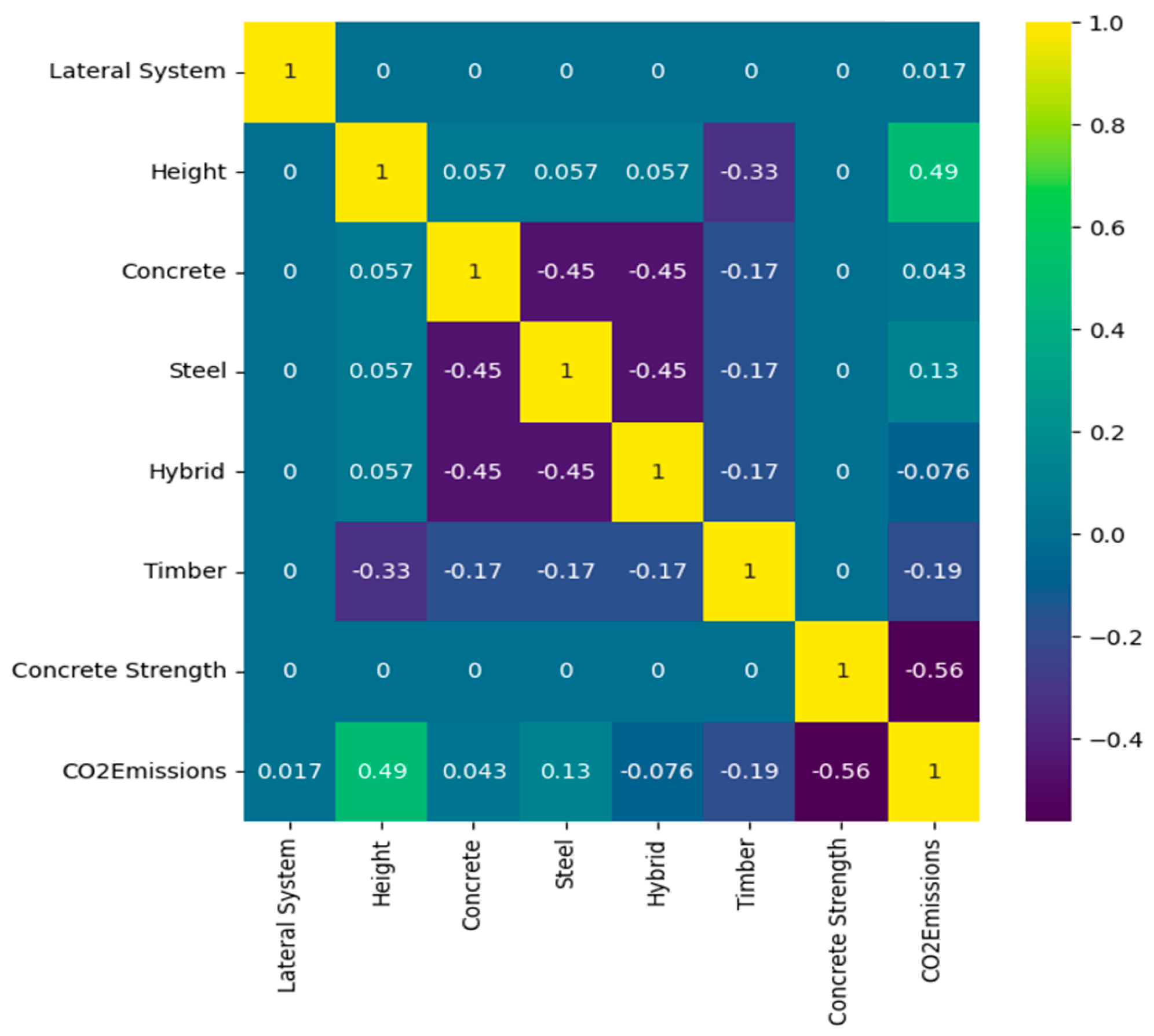
Figure 8 displays the correlation matrix, providing a graphical summary of all Pearson correlation coefficient (r) values for the features in this study. The correlation coefficient (r) quantifies the linear relationship between two variables. A value of r = 0 indicates no linear trend between the variables. A positive correlation (r > 0) suggests that as one variable increases or decreases, so does the other; a value closer to 1 signifies a stronger relationship. Conversely, a negative correlation (r < 0) indicates that as one variable increases, the other decreases, and vice versa. In our analysis, It was observed a strong relationship between height and CO₂ emissions (CO₂-e), followed by steel and concrete. This indicates that these variables have the most significant impact on CO₂ emissions in tall buildings. Other variables, such as concrete strength, timber, and hybrid systems, exhibit comparatively weaker impacts.

Therefore, using a hybrid system and higher strength concrete in designing tall buildings would lead to reduced CO2 emissions and less environmental impact.

5. Conclusions

This research presents a data driven-based approach focusing on decarbonization of tall buildings. It evaluates the significant impact of material types (concrete, steel, and timber), concrete strength, and structural systems relative to a building’s height on the EGHGE associated with tall buildings. A wide spectrum of tall buildings was considered in this study encompassing: four different types of lateral structural systems (Braced-Frame system, Outrigger-Belt system, Shear Wall system, and Tubular system), four different types of construction materials (concrete, steel, hybrid, and timber), varying heights (ranging from 10 to 100 stories), and various concrete materials with different compressive strength ranging from 32 to 90 MPa. Data from FEM simulations along with data from existing projects were used to train four ML regression methods and the best model was selected to accurately predict the total amount of CO₂ emissions of tall buildings.

ML results showed that the decision tree regression model exhibited the highest predictive performance, followed by the polynomial regression model. Results also demonstrated that the hybrid structures consistently had lower carbon emissions compared to concrete and steel structures. Furthermore, timber structures exhibited the lowest embodied carbon for buildings below 20 stories. Overall, hybrid structures with the Out-Rigger-Belt system displayed the most favorable CO₂ emission patterns across different story levels and lateral systems. Additionally, findings indicated that tall buildings constructed with high-strength concrete (60+ MPa) consistently exhibited lower CO₂ emissions, particularly in hybrid structures containing the Out-Rigger-Belt system.

Author Contributions

Conceptualization, [PA] and [BB]; methodology, [PA]; software, [PA]; validation, [PA] and [BB]; formal analysis, [PA]; investigation, [PA]; resources, [PA]; data curation, [PA]; writing—original draft preparation, [PA]; writing—review and editing, [PA] and [BB]; visualization, [PA]; supervision, [PA]; project administration, [PA]; funding acquisition, [PA]. All authors have read and agreed to the published version of the manuscript.

Funding

This research received no external funding and was entirely self-funded by the authors.

Data Availability Statement

The data presented in this study include results from various analyses and FEM models, some of which are based on confidential projects and cannot be shared publicly. However, additional FEM models and associated data, including Excel sheets of the results, are available from the corresponding author upon reasonable request.

References

De La Peña, B., Iriondo, A., Galletebeitia, A., Gutierrez, A., Rodriguez, J., Lluvia, I., & Vicente, A. (2023). Toward the Decarbonization of the Steel Sector: Development of an Artificial Intelligence Model Based on Hyperspectral Imaging at Fully Automated Scrap Characterization for Material Upgrading Operations. Steel Research International, 94(11), 2200943. [CrossRef]
De Wolf, C. (2014). Material quantities in building structures and their environmental impact.
Fraga-De Cal, B., Garrido-Marijuan, A., Eguiarte, O., Arregi, B., Romero-Amorrortu, A., Mezzasalma, G., Ferrarini, G., & Bernardi, A. (2021). Energy Performance Assessment of Innovative Building Solutions Coming from Construction and Demolition Waste Materials. Materials, 14(5), 1226. [CrossRef]
Giannelos, S., Moreira, A., Papadaskalopoulos, D., Borozan, S., Pudjianto, D., Konstantelos, I., Sun, M., & Strbac, G. (2023). A Machine Learning Approach for Generating and Evaluating Forecasts on the Environmental Impact of the Buildings Sector. Energies, 16(6), 2915. [CrossRef]
Hamelin, M.-C., & Zmeureanu, R. (2014). Optimum Envelope of a Single-Family House Based on Life Cycle Analysis. Buildings, 4(2), 95–112. [CrossRef]
Helal, J., Stephan, A., & Crawford, R. (2018). Beyond the “premium-for-height” framework for designing structural systems for tall buildings: Considering embodied environmental flows.
Helal, J., Stephan, A., & Crawford, R. H. (2019). Towards a design framework for the structural systems of tall buildings that considers embodied greenhouse gas emissions. In P. J. S. Cruz (Ed.), Structures and Architecture: Bridging the Gap and Crossing Borders (1st ed., pp. 881–888). CRC Press. [CrossRef]
Helal, J., Stephan, A., & Crawford, R. H. (2020). The influence of structural design methods on the embodied greenhouse gas emissions of structural systems for tall buildings. Structures, 24, 650–665. [CrossRef]
Jiwei Li, L. X. (2020). Advances in the Study of Building Energy Consumption by Machine Learning Method. Computer Science and Application, 10(05), 1002–1008. [CrossRef]
Lavercombe, A., Huang, X., & Kaewunruen, S. (2021). Machine Learning Application to Eco-Friendly Concrete Design for Decarbonisation. Sustainability, 13(24), 13663. [CrossRef]
Płoszaj-Mazurek, M. (2020). Machine Learning-Aided Architectural Design for Carbon Footprint Reduction. BUILDER, 276(7), 35–39. [CrossRef]
Sanni-Anibire, M. O., Mohamad Zin, R., & Olatunji, S. O. (2021). Developing a preliminary cost estimation model for tall buildings based on machine learning. International Journal of Management Science and Engineering Management, 16(2), 134–142. [CrossRef]
Shang, M., Li, H., Ahmad, A., Ahmad, W., Ostrowski, K. A., Aslam, F., Joyklad, P., & Majka, T. M. (2022). Predicting the Mechanical Properties of RCA-Based Concrete Using Supervised Machine Learning Algorithms. Materials, 15(2), 647. [CrossRef]
Behzad Behnia, Peyman Askarinejad, Noah LaRussa-Trott (2023). Investigating Low-Temperature Cracking Behavior of Fiber Reinforced Asphalt Concrete Materials.

Figure 1. (a). This is a figure of CO₂ emissions of concrete structure with shear wall system. (b). This is a figure of CO₂ emissions of concrete structure with braced frame system. (c). This is a figure of CO₂ emissions of concrete structure with out-rigger system. (d). This is a figure of CO₂ emissions of concrete structure with Tube system.

Figure 2. The rate of change in CO₂ emissions vs. height of tall buildings.

Figure 3. (a). This is a figure of CO₂ emission of steel structure with a shear wall system. (b). This is a figure of CO₂ emission of steel structure with a braced-frame system. (c). This is a figure of CO₂ emission of steel structure with out-rigger system. (d). This is a figure of CO₂ emission of steel structure with a tube system.

Figure 4. (a). CO₂ emission of tall buildings with hybrid materials and shear wall system. (b). CO₂ emission of tall buildings with hybrid materials and braced-frame system. CO₂ emission of tall buildings with hybrid materials and out-rigger system. (d). CO₂ emission of tall buildings with hybrid materials and tube system.

Figure 5. (a). CO₂ emission in concrete, steel, and hybrid structures with 60 MPa concrete in shear wall lateral system. (b). CO₂ emission in concrete, steel, and hybrid structures with 60 MPa concrete in out-rigger lateral system.

Figure 6. (a). CO₂ emission of concrete and hybrid structures with different concrete strength for out-rigger lateral system. (b). CO₂ emission of concrete and hybrid structures with different concrete strength for tube lateral system.

Figure 8. Pearson correlation matrix used for feature selection in regression analysis.

Disclaimer/Publisher’s Note: The statements, opinions and data contained in all publications are solely those of the individual author(s) and contributor(s) and not of MDPI and/or the editor(s). MDPI and/or the editor(s) disclaim responsibility for any injury to people or property resulting from any ideas, methods, instructions or products referred to in the content.

© 2024 by the authors. Licensee MDPI, Basel, Switzerland. This article is an open access article distributed under the terms and conditions of the Creative Commons Attribution (CC BY) license (http://creativecommons.org/licenses/by/4.0/).

Copyright: This open access article is published under a Creative Commons CC BY 4.0 license, which permit the free download, distribution, and reuse, provided that the author and preprint are cited in any reuse.

MDPI Initiatives

Important Links

Choose an area of interest and we will send you notifications of new preprints at your preferred frequency.

Disclaimer

Decarbonizing Tall Building Structures: Implementing Machine Learning At The Early-stage Of Design Process

Abstract

1. Introduction

2. Methodology

2.1. Notions and Definitions

2.1.1. Tall Buildings

2.1.2. Structural Systems

2.2. Data Collection and Determination of Global Warming Potential (GWP)

3. Finite Element Modeling of Tall Buildings

4. Implementation of Machine Learning Methods

4.1. Elastic-Net Regularized Regression Method

4.2. Polynomial Regression (PR) Method

4.3. Decision Tree Regression Method

4.4. Support Vector Regression (SVR) Method

4.5. Performance Evaluation of ML Models

4.6. ML-Based CO2 Prediction Model

4.7. Pearson Correlation Method

5. Conclusions

Author Contributions

Funding

Data Availability Statement

References

MDPI Initiatives

Important Links

Subscribe