3.1. Optimization of indoor 3D reconstruction based on adaptive normal prior
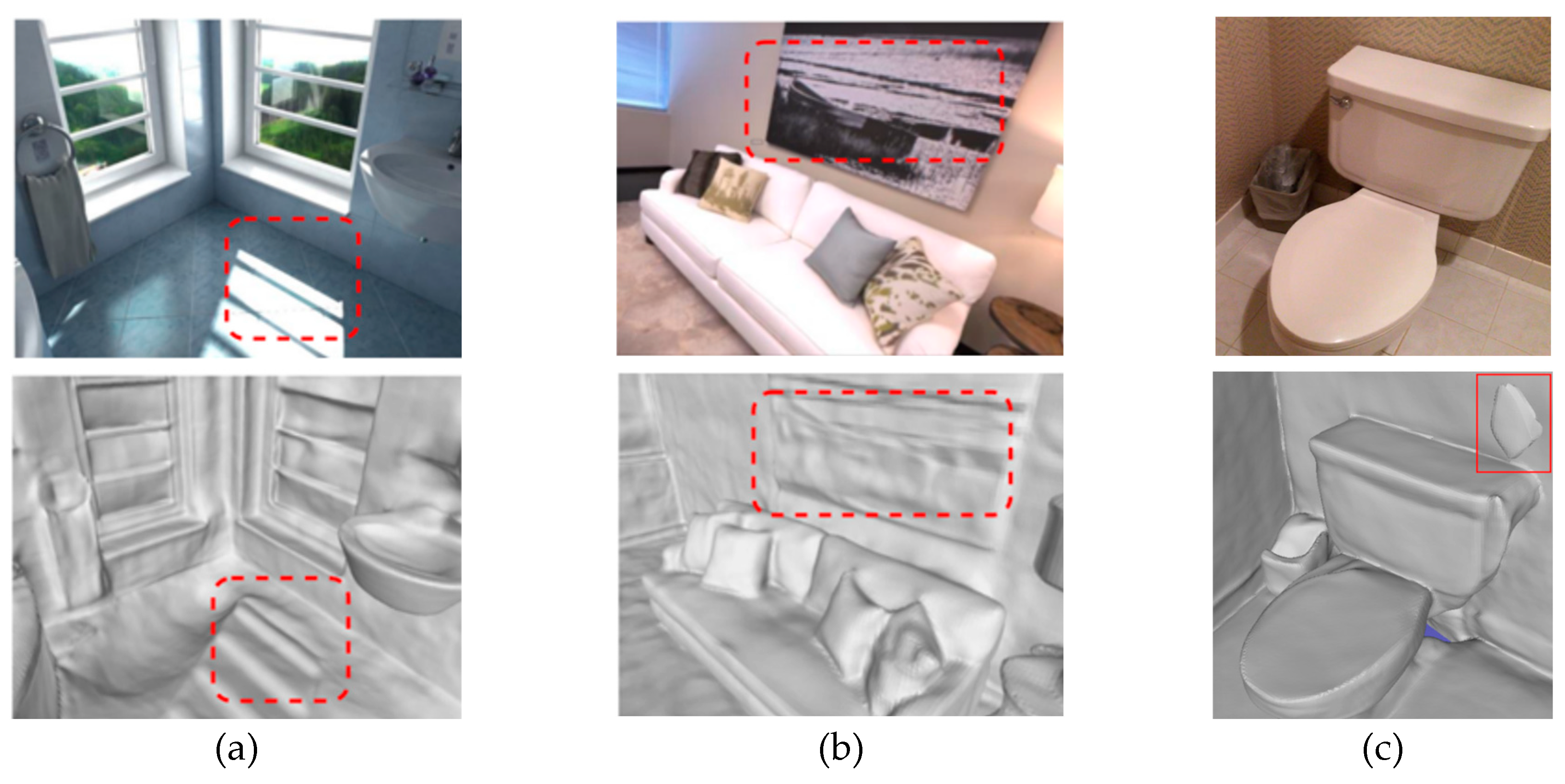
Normal map is an important type of image, which represents the surface normal direction of each pixel in the image through the color of the pixel. In 3D graphics and computer vision, the normal is a vector perpendicular to the surface of an object, which can be used to describe the direction and shape of the surface. In the normal map, RGB color channels are generally used to represent the X, Y, and Z components of the normal vector respectively. Normal information helps to correct errors in the reconstruction process and improve the reconstruction quality.
Currently, many monocular normal estimation methods have achieved high accuracy under clear image input. However, considering that indoor scene images often have small blur and tilt, this paper selects TiltedSN [
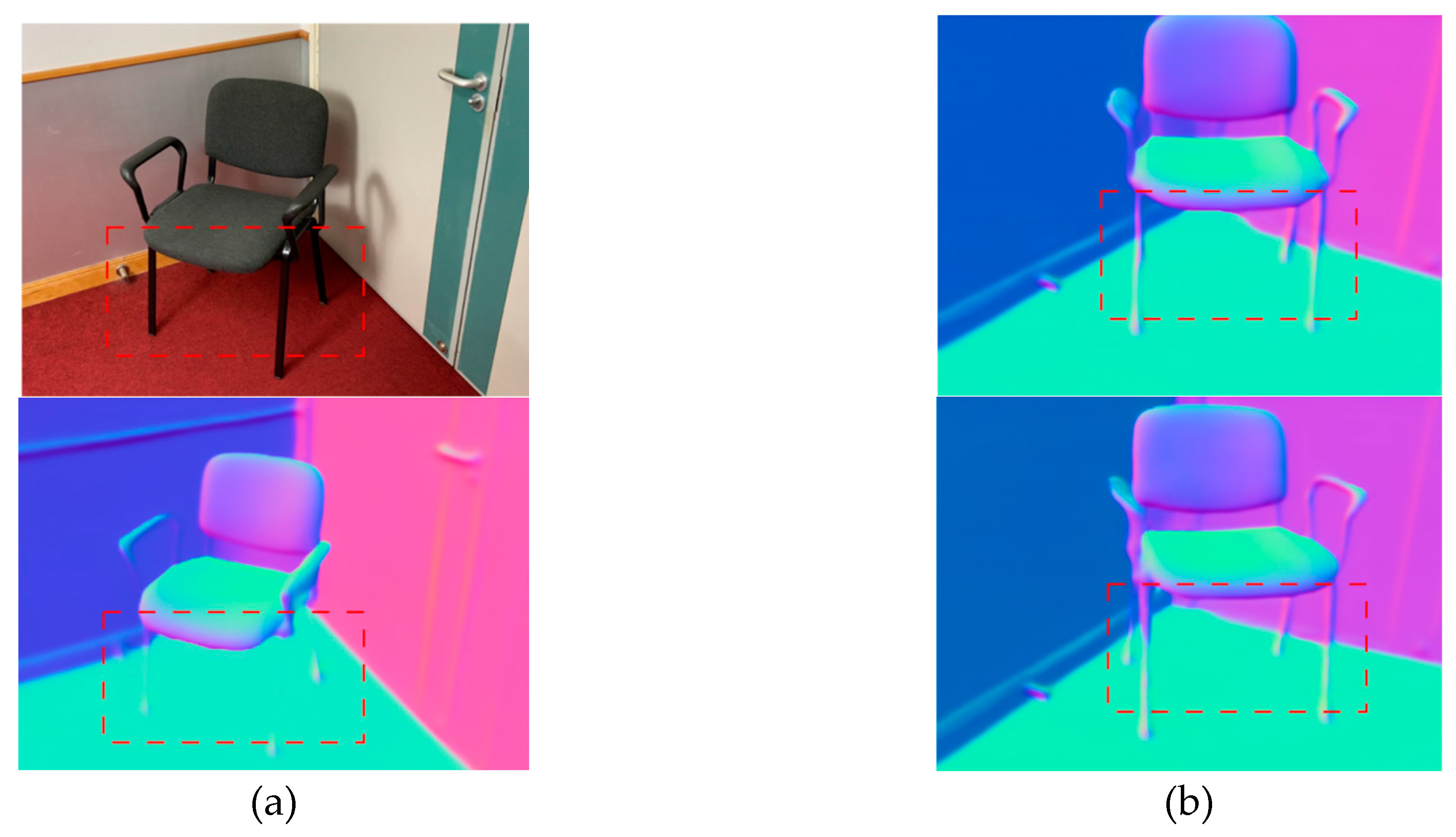
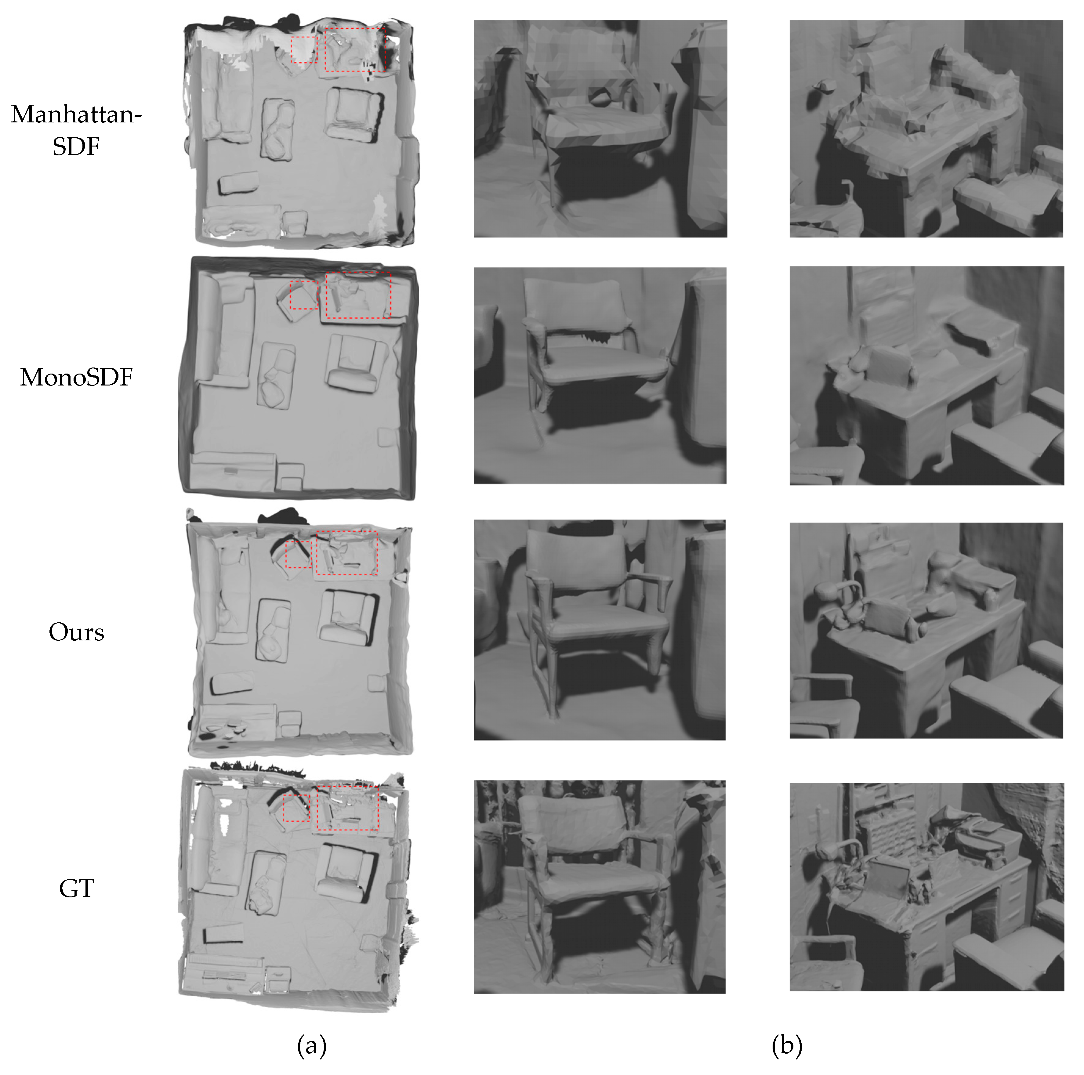
20] as the normal estimation module. Because the estimated normal map is usually over-smoothed, there are problems of inaccurate estimation on some fine structures, such as the chair legs in
Figure 3(a). Therefore, we adopt an adaptive method to use normal priors, using a mechanism based on the consistency of multiple views of the input image to evaluate the reliability of the normal prior. As shown in
Figure 3(b), this process is also called geometric checking. For areas that do not meet the consistency of multiple images, the normal prior is not applied. Instead, the appearance information is used for optimization to avoid the negative effects of incorrect normal maps that lead to misjudgment in reconstruction.
Given a reference image
, evaluate the consistency of the surface observed from pixel
. Define a local 3D plane
in the camera space associated with
, where
is the viewing direction,
is the distance to pixel
, and
is the normal estimate. Next, find a set of adjacent images, assuming that one of the adjacent images is
. The homography change from
to
can be calculated by the following formula:
where
is the intrinsic parameter matrix, the rotation and translation camera parameters. For pixel
in
, find a square block
centered on it as the neighborhood, and warp the block to its adjacent view
using the calculated homography matrix. The block matching method (Patchmatch) can be used to find similar image blocks on adjacent views, and the Normalized Cross-Correlation (NCC) method is used to evaluate the visual consistency of (
,
). NCC is a method for measuring the similarity between two images. It evaluates the similarity between the two images by calculating the degree of correlation between them. Compared with simple cross-correlation, normalized cross-correlation is insensitive to changes in brightness and contrast, so it is more reliable in practical applications. The applied NCC formula is as follows:
where
,
and
represent two image regions to be compared,
is the average value of
,
is the difference between them, the numerator calculates the sum of the products of the differences between the two image blocks, and the denominator calculates the square root of the product of the sum of the squares of the differences between the two image blocks. This process ensures the normalization of the results, making the NCC range in (-1, 1). The closer the NCC value is to 1, the more similar the two image regions are; the closer the NCC value is to -1, the less similar they are; the closer the NCC value is to 0, the less obvious linear relationship there is between them.
If the reconstructed geometry is not accurate at the sampling pixel, it cannot meet the multi-view photometric consistency, which means that its related normal prior cannot provide help for the overall reconstruction. Therefore, a threshold ϵ is set, and by comparing the NCC at the sampling block with ϵ, the following indicator function can be used to adaptively determine the training weight of the normal prior.
The normal prior is used for supervision only when . If , the normal prior of the region is considered unreliable and will not be used in subsequent optimization processes.
3.2. Neural implicit reconstruction
Since the neural radiation field cannot express the surface of the object well, we are looking for a new implicit expression. The signed distance function (SDF) can represent the surface information of objects and scenes and achieve better surface reconstruction. Therefore, we choose SDF as the implicit scene representation.3.3.1 Scene Representation
3.2.1. Scene Representation
We represent the scene geometry as a SDF. A SDF is a continuous function f that, for a given 3D point, returns the distance from that point to the nearest surface:
Here,
represents a 3D point and
is the corresponding SDF value, thus completing the mapping from a 3D point to a signed distance. We define the surface
as the zero level set of the SDF, expressed as follows:
By using the Marching Cubes algorithm on the zero horizontal plane of the SDF, that is, the surface of the object or scene, we can obtain a 3D mesh with a relatively smooth surface.
Using the SDF to get the mesh has the following advantages:
1) Clear surface definition: SDF provides the distance to the nearest surface for each spatial point, where the surface is defined as the location where the SDF value is zero. This representation is well suited for extracting clear and precise surfaces, making the conversion from SDF to mesh relatively direct and efficient.
2) Geometric accuracy: SDF can accurately represent sharp edges and complex topological structures, which can be maintained when converted to meshes, thereby generating high-quality 3D models.
3) Optimization-friendly: The information provided by SDF can be directly used to perform geometry optimization and mesh smoothing operations, which helps to further improve the quality of the model when generating the mesh.
3.2.2. Implicit indoor 3D reconstruction based on normal prior
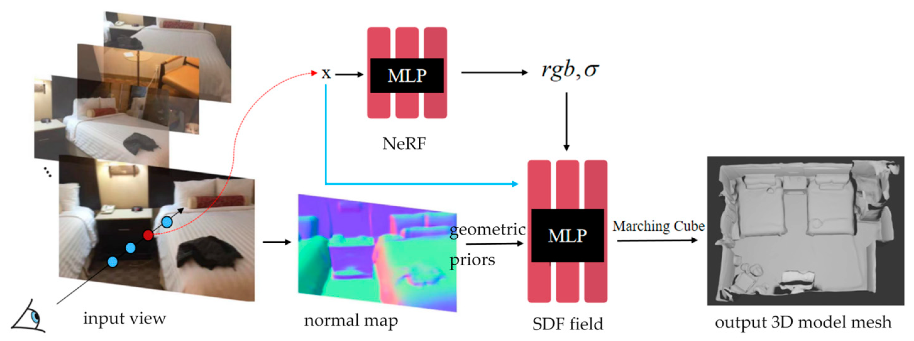
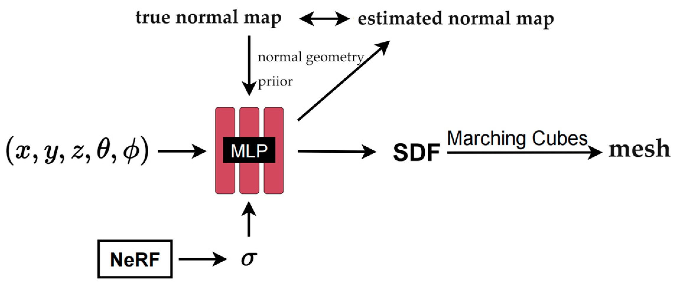
The reconstruction process based on normal prior is shown in
Figure 4. The input mainly consists of three parts.
The first part is a five-dimensional vector representing the information of the sampling point . The second part is the volume density we obtained previously through the neural radiation field . Given that we use SDF as a surface expression, the volume density obtained by NeRF can represent more comprehensive scene geometry information. Because the scene contains multiple objects and air, it is difficult to represent a complex scene only through surface information. Traditional SDF-based methods are often limited to object reconstruction. The constraints of NeRF volume density combined with SDF reconstruction can reconstruct richer scene geometry. The third part is the normal geometry prior. The normal map here is obtained by the monocular normal estimation method mentioned earlier. The normal map provides the orientation information of the object surface, which is conducive to enhancing detail reconstruction.
The network used here is an improved neural radiation field, which also contains 2 MLPs. Like NeRF, there is a color network , and the other grid has become an SDF network , which can get the SDF value of the point through the 3D coordinates of the point.
Here we will use volume rendering technology to get the predicted image, and optimize it with the input real image through the loss function. Specifically, for each pixel, we sample a set of points along the corresponding emission light, denoted as
, where
is the sampling point,
is the camera center, and
is the direction of the light. The color value can be accumulated by the following volume rendering formula.
where
is the cumulative transmittance, i.e., the probability that of no object occlusion, c is the color value,
is the discrete opacity, and
is the opacity corresponding to the volume density
in the original NeRF. Since the rendering process is fully differentiable, we learn the weights of
and
by minimizing the difference between the rendering result and the reference image.
In addition to generating the appearance, the above volume rendering scheme can also obtain the normal vector. We can approximate the surface normal observed from a viewpoint by volume accumulation along this ray:
where
is the gradient at point
.
At this time, we compare the true normal map obtained by the monocular method with the estimated normal map obtained by the volume rendering process, and further optimize the parameters of the MLP by calculating the loss to obtain a more accurate normal map and geometric structure.
3.3. Floating debris removal
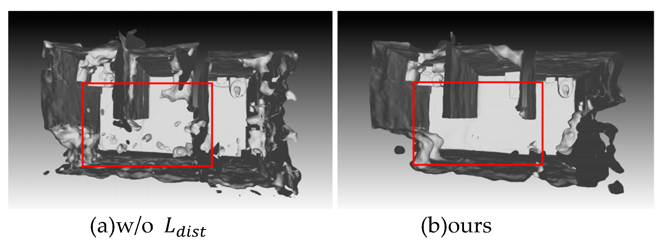
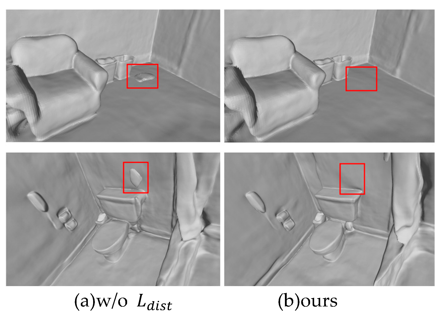
The neural radiation field initially acts on the generation of new perspectives on objects, maintaining a high degree of clarity and realism. This is mainly due to volume rendering. However, when the neural radiation field is used for 3D reconstruction, some floating debris in the air often appear. These floating debris refer to small disconnected areas in the volume space and translucent substances floating in the air. In view synthesis work, these floating debris are often not easy to detect. However, if an explicit 3D model needs to be generated, these floating debris will seriously affect the quality and appearance of the 3D model. Therefore, it is very necessary to remove the floating debris in these incorrectly reconstructed places.
These floating debris often do not appear in object reconstruction. However, in scene-level reconstruction, due to the significant increase in environmental complexity and the lack of relevant constraints on the neural radiation field, there is a phenomenon of inaccurate local area density prediction. Therefore, this paper proposes a new regularization term to constrain the weight distribution of the neural radiation field.
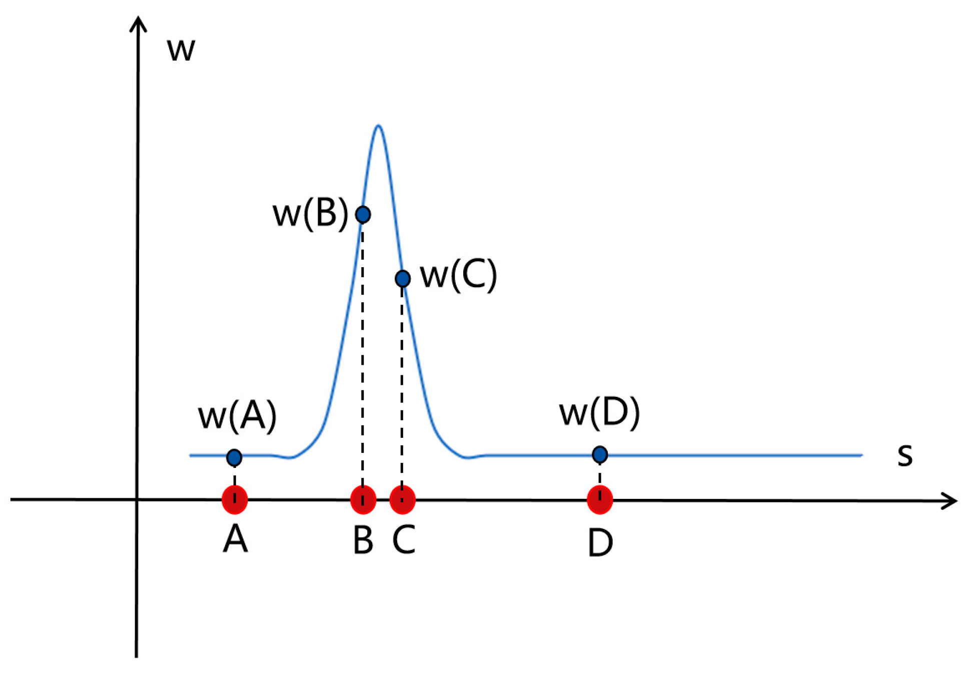
First, simulate the sampling process of the neural radiation field. In a scene, assume that there are only rigid objects, excluding the existence of translucent objects. After a ray is shot out, there will be countless sampling points on this ray. The weight value of the sampling point before the ray encounters the object should be extremely low (close to 0). When the ray contacts the rigid object, the weight value here should soar, much higher than other values. After the object, the weight value returns to a lower range. This is the desired weight distribution in an ideal state, which is a relatively compact unimodal distribution. This method defines a regularization term, which is a step function defined by a set of standardized ray distances s and the weight w after parameterizing each ray:
Here and refer to points on the sampling ray, that is, points on the x-axis in the weight distribution diagram, is the distance between the two points, and are the weight values at point u and point v, respectively. Since all particle combinations from negative infinity to positive infinity need to be exhausted, integration is performed in the front. If you want to make the loss function as small as possible, there are mainly two situations:
1) If the distance between point u and point v is relatively far, that is, the value of
is large, if you want to ensure that the value of
is as small as possible, then one of
and
needs to be small and close to zero. That is, as shown in
Figure 5, (A, B), (B, D), (A, D), etc. all satisfy that
is large and the weight value of at least one point is extremely small (close to zero);
2) If the values of and are both large, if you want to ensure that the value of is as small as possible, then the value of needs to be small, that is, the distance between points u and v is very close. As shown in figure 5, only the combination of (B, C) satisfies the condition that the values of and are both large, and at this time, points and just meet the condition that the distance is very close.
Therefore, through the analysis of the above two cases, it can be found that the properties of the regularization term can constrain the density distribution to the ideal single-peak distribution with good central tendency proposed before. The purpose of this regularization term is to minimize the sum of the normalized weighted absolute values of all samples along the ray, and encourage each ray to be as compact as possible, which is specifically reflected in:
1. Minimize the width of each interval;
2. Bring the intervals that are far apart closer to each other;
3. Make the weight distribution more concentrated.
The regularization term above cannot be used directly for calculation because it is in integral form. In order to facilitate calculation and use, it is discretized as:
This discretized form also provides a more intuitive understanding of the behavior represented by this regularization, where the first term minimizes the weighted distance between points in all intervals, and the second term minimizes the weighted size of each individual interval.
3.4. Training and loss function
During the training phase, we sample a batch of pixels and adaptively minimize the difference between the color and normal estimates and the true normal map. We sample
pixels
and their corresponding reference colors
and normals
in each iteration. For each pixel, we sample
points in the world coordinate system along the corresponding ray, and the total loss is defined as:
Among them , , and are the hyperparameters of color loss, normal loss, Eikonal loss and distortion loss respectively.
Color loss
is used to measure the difference in color between the reconstructed image and the real image:
In the training phase, a batch of pixels need to be sampled. Each iteration samples pixels {} and the corresponding reference color {}, where represents the pixel color predicted by volume rendering.
The normal prior loss
is to render the reconstructed 3D mesh of the indoor scene as a normal map, and compare it with the real normal map generated by the monocular method to obtain a loss:
where
is the true normal information, and
is the normal information predicted by the gradient.
is an indicator function used to judge the accuracy of the normal prior. Here, some data with inaccurate normal estimation are eliminated. The normal loss is mainly calculated by cosine similarity, because the direction of the normal vector is more important than its length. Cosine similarity is a good measure of the similarity of the two vectors in direction.
The Eikonal loss
[31] of the regularized SDF is
where
is a set of sampling points in the 3D space and the area near the surface, and
represents one of the sampling points. The reason why the gradient
needs to be close to 1 is that the ideal SDF represents the shortest distance from the current point to the surface, so the gradient direction is the direction in which the distance field changes the steepest. Assuming that x moves toward the surface along this direction by ∆d, the SDF should also change by ∆d. Therefore, in the ideal state,
, where
is the original Eikonal equation. By introducing the Eikonal loss, the properties of the SDF can be well constrained, thereby ensuring the smoothness and continuity of the reconstructed surface.
