Preprint
Article

Addressing Low-Cost Methane Sensor Calibration Shortcomings with Machine Learning

Altmetrics

Downloads

97

Views

74

Comments

0

A peer-reviewed article of this preprint also exists.

Submitted:

27 August 2024

Posted:

29 August 2024

You are already at the latest version

Alerts
Abstract
Quantifying methane emissions is essential for meeting near-term climate goals and typically done using methane concentrations measured downwind of the source. One major source of methane that is important to observe and promptly remediate is fugitive emissions from oil and gas productions sites but installing methane sensors at the thousands of sites within a production basin is expensive. In recent years, relatively inexpensive metal oxide sensors have been used to measure methane concentrations at production sites. Current methods used to calibrate metal oxide sensors have been shown to have significant shortcomings resulting in limited confidence in methane concentrations generated by these sensors. To address this, we investigate using machine learning (ML) to generate a model that converts metal oxide sensor output to methane mixing ratios. To generate test data, two metal oxide sensors, TGS2600 and TGS2611, were collocated with a trace methane analyzer downwind of controlled methane releases. Over the duration of the measurements, the trace gas analyzer’s average methane mixing ratio was 2.40 ppm with a maximum of 147.6 ppm. The average calculated methane mixing ratios for the TGS2600 and TGS2611 using the ML algorithm were 2.42 ppm and 2.40 ppm with maximum values of 105.9 ppm and 106.3 ppm, respectively. A comparison of histograms generated using the analyzer and metal oxide sensors mixing ratios show overlap coefficients of 0.95 and 0.94 for the TGS2600 and TGS2611, respectively. Overall, our results showed there was a good agreement between the ML derived metal oxide sensors’ mixing ratios and those generated using the more accurate trace gas analyzer. This suggests that the response of lower-cost sensors calibrated using ML could be used to generate mixing ratios with precision and accuracy comparable to higher price trace methane analyzers. This would improve confidence in low-cost sensors’ response, reduce the cost of sensor deploying, and allow for timely and accurate tracking of methane emissions.
Keywords: 
Subject: Environmental and Earth Sciences  -   Pollution

1. Introduction

Methane (CH4), a gas with a global warming potential 25 times greater than carbon dioxide, has increased in atmospheric composition by a factor of three since preindustrial times largely due to changes in emissions from anthropogenic activities [1,2]. Nearly all countries globally have entered treaties or agreements to reduce methane emissions but it has recently been suggested that methods used to quantify methane emissions are insufficiently precise to measure emission reduction of mitigation strategies [3,4,5,6].
Measuring methane emissions from oil and gas production activities has been the focus of many studies since the 1990s [7,8,9,10,11,12]. Recently, approaches have developed from survey methods, where short-duration measurements are made by instruments mounted on a mobile platform [13,14,15], to continuous monitoring approaches, where measurements are made by instrumentation fixed in location [6,16,17,18]. The advantage of continuous monitors is that observations are more likely to detect the short-duration, large-emission events that are typical of oil and gas emission distributions and are essential to capture if realistic emissions estimates are to be generated [19,20]. Typically, on-site continuous monitoring systems comprise of several (minimum of four) methane measurement/meteorological instrumentation installed at fixed points around the site coupled with a dispersion model to infer a rate of emission [6,21,22]. One difficulty in designing a continuous monitoring system that is to be installed at the fence line of an oil and gas production site is the choice of methane measurement instrumentation. Methane sensing technologies include metal oxide sensors ($15 per sensor), integrated infra-red sensors ($300 per sensor), tunable diode laser absorption spectrometers ($1000 per sensor) and optical cavity instrumentation (> $10,000 per sensor). As there are thousands of productions sites across the US alone, costly (> $1,000) methane measurement systems are prohibitively expensive to deploy at every site therefore metal oxide sensors are currently being widely deployed across oil and gas production sites across the US [6,22].
As metal oxide sensors are being widely distributed to measure near-background methane concentrations in air (typically below 100 ppm), many studies have described methods of calibration, deployment and response, however, most studies report that these sensors are sensitive to temperature and relative humidity and required individual calibration [17,23,24,25,26,27,28,29,30]. Typical metal oxide sensor models used in these studies are the Taguchi Gas Sensors (TGS) 2600 and 2611 models produced by Figaro Engineering Inc. (Osaka, Japan). TGS2600 uses a tin-dioxide (SnO2) sensing layer that reacts with the detected gases. The detection mechanism relies on the change in electrical conductivity through the SnO2 in presence of methane which is a reducing gas. Absorbance of oxygen molecules occurs on the surface of SnO2 forming O2- ions leading to electron capture that creates a depletion layer at the surface of the SnO2 increasing its resistance [23,24]. Methane interacts with the adsorbed oxygen ions releasing the trapped electrons back into the SnO2 conduction band, decreasing its resistance. The change in resistance is proportional to the concentration of CH4. The TGS2611 has the same operation basis as the TGS2600 but has been optimized for methane detection by the integration of a heating element to maintain optimal temperature for methane detection and features a filter material that selectively permits methane to reach the sensing element while blocking other gases [23,24].
Studies using Figaro TGS sensors have measured the resistance change across the metal oxide strip to infer changes in concentration. It is assumed the metal oxide sensor has a relatively constant resistance in clean air (R0, Ω) which becomes lower in the presence of methane (Rs, Ω) and the ratio of these resistances gives a measure of the methane mixing ratio in air. The resistance of the metal oxide sensor is also affected by the air temperature (Ta, °C) and relative humidity (rH, %) and the ratio of resistance can be corrected to account for these factors using an empirically derived algorithm (Equation (1)) [25].
R s R 0 c o r r = R s R 0 . 0.024 + 0.0072 . r H + 0.0246 . T a
The temperature and humidity corrected ratio of Rs and R0 is then typically converted to a methane mixing ratio using a sensor-specific calibration algorithm [25,30]. As they perform badly in low relative humidity, less than 40% RH [30], the TGS sensors are typically calibrated by comparing (Rs/R0)corr to methane mixing ratios measured using a sub-ppm reference instrument measuring methane contemporaneously. An algorithm is then generated to translate (Rs/R0)corr to a calibrated mixing ratio ([CH4]cal). Published algorithms have been linear, power functions and exponential functions [17,23,25,26,30,31] and there is not a good current understanding of differences between individual sensors’ response to changing methane concentrations apart from possible differences in manufacturing [17].
Nested within the conversion from measured data to a calibrated methane mixing ratio are several potential sources of uncertainty: 1. The size of the measured resistance (Rs) appears to be highly variable between individual sensors and through trial and error, we have found that the output of some of the sensors in near background mixing ratios (< 10 ppm)- the methane signal has become almost indistinguishable from the noise; 2. The calculation of [CH4]cal is heavily dependent on determining a value for the TGS resistance in clean air, R0; 3. Given the variability in response of sensors to changes in methane concentration, it seems questionable that all sensors would respond equally to changes in relative humidity and temperature (as defined in Equation (1)) especially in sensors with low signal to noise ratios. Overall, these uncertainties raise concerns about the historical methods for converting signals from TGS methane sensors to a calibrated methane mixing ratio.
One alternative approach could be to use a novel machine learning approach that accounts for low signal to noise ratios and differences in sensor response to relative humidity and temperature changes. Recent developments in machine learning algorithms have transformed sensor calibration and enhanced their reliability in environmental monitoring [32]. One example of machine learning is the Random Forest (RF) Regressor developed by Leo Breiman in 2001. Random Forest is an ensemble machine learning model [35], which implies that the model is built by the combination of predictions from multiple simpler models [33]. Random Forest uses a collection of decision trees which are the models that split the data into branches based on the input features to make a prediction. Training the RF regression model involves presenting the model with the input variables (metal oxide sensors’ resistances, temperature and relative humidity) that are passed through multiple decision trees and the output aggregation predict the target variable (in this case the trace gas analyzer CH4 concentrations).
To investigate this, we will use two TGS sensors with low signal to noise ratio and report on the RF machine learning approach to generating calibrated methane mixing ratios. Specifically, we will 1. Collect Rs values from low-response TGS2600 and TGS2611 sensors contemporaneously with a sub-ppm methane analyzer; 2. Generate calibrations curves using (a) the traditional method (presented above) and (b) RF machine learning approach; and 3. compare the calibrated methane mixing ratios reported by the TGS2600 and TGS2611 to the methane analyzer to generate an understanding of sensor type response, bias and drift over time. Ultimately, we aim to provide evidence to understand if the RF machine learning approach can generate better calibration algorithms than currently used methods.

2. Materials and Methods

2.1. Methane Measurement

2.1.1. Figaro TGS Sensors
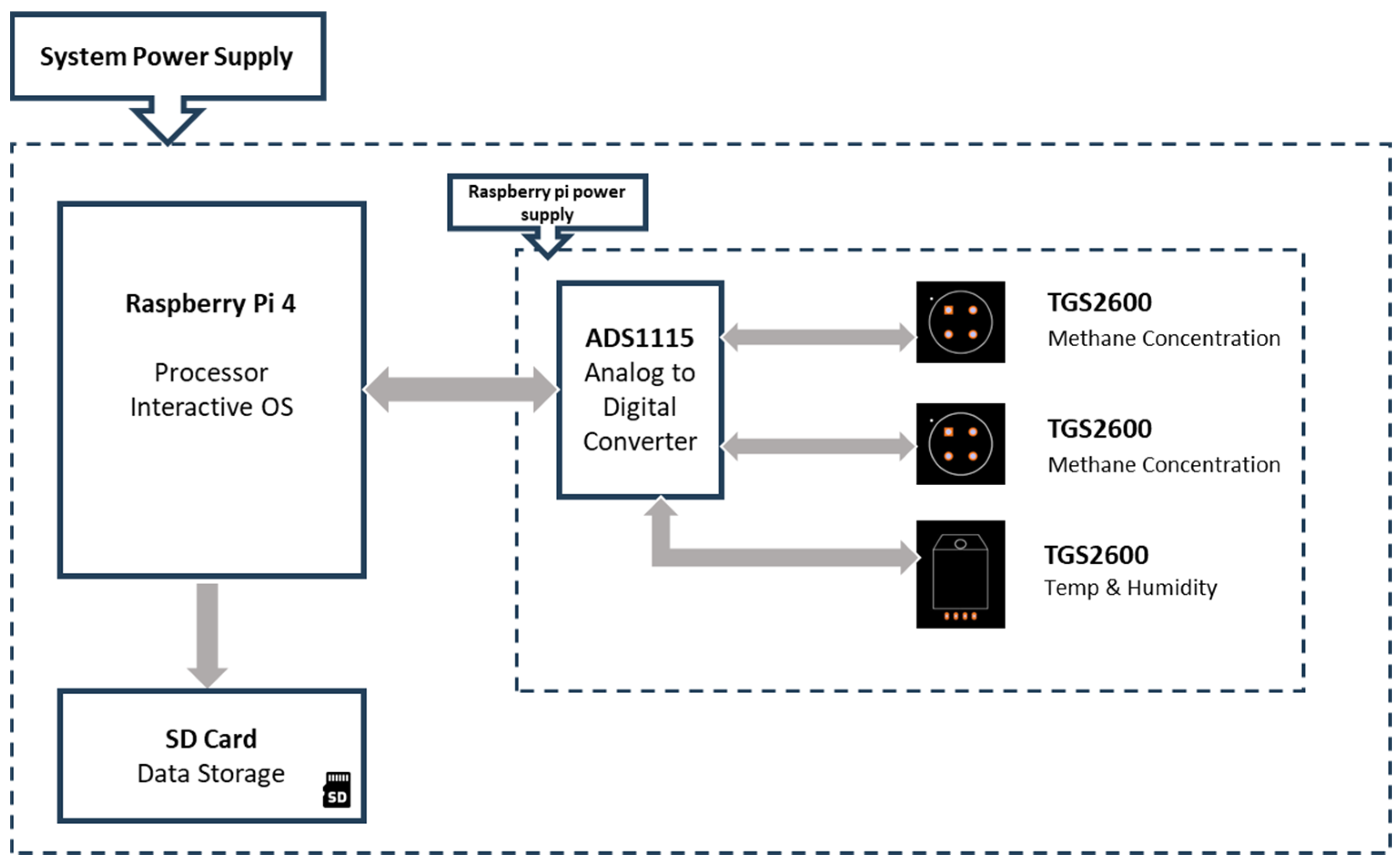
Both the TGS 2600 and 2611 sensors were connected to a Raspberry Pi 4 (London, UK) via an ADS1115 16-Bit analog to digital converter, with an inclusion of DHT22 temperature and humidity sensor. The Raspberry Pi was powered by a 5V 3A USB-C power supply adapter and the sensors were powered by the Raspberry pi’s MaxLinear MxL7704 regulator. The TGS 2600, 2611 and DHT22 were connected to the A0, A1 and A2 pin of the module, respectively. The sensors sampled at a height of 2m. A python script was used to enable continuous reading of data at 1s intervals. The script leveraged the Inter-Integrated Circuit (I2C) communication protocol to interface with the ADS1115, deploying the Adafruit ADS1x15 library for data acquisition. The acquired data was timestamped and written to daily individual files.
Figure 1. System architecture of the Figaro TGS2600 and Figaro TGS2611 metal oxide sensors.
Preprints 116447 g001

2.1.2. Reference instrument—Aeris MIRA Ultra Mobile LDS

The Aeris Technologies, Inc. (Hayward, CA, USA) Ultra is a mid-infrared laser absorption analyzer [34]. This instrument integrates a laser absorption spectrometer operating in the mid-infrared spectrum achieving simultaneous quantification of methane between 10 ppb and 10,000 ppm and ethane between 1 ppb and 1,000 ppm. [34]. The device operates at standard rates of 1 or 2 Hz, with an option to increase it to 10 Hz. For these experiments, the instrument was set to measure at 5Hz.

2.2. Controlled Methane Release Experiments

Controlled methane release experiments were conducted at Colorado State University’s Methane Emission Technology evaluation Center (METEC) in Fort Collins, CO between March 1st, 2024, and 2nd May 2024. Natural gas of a known composition was released from single and multiple above-ground points on well heads, separators and tanks on Pads 4 and 5 at emissions rates of between 0.005 and 8 kg CH4 h-1 (Figure 2). The TGS sensors and the inlet to the Aeris Sentinel analyzer were collocated (40.60° N, 105.14° W) on the north-west of the site at 2m above ground level. During the deployment period, the external temperatures ranged from -22oC in the early weeks of deployment to 30oC in the later stages.

2.3. Eugster and Kling (2012) Metal Oxide Sensor Calibration

A calibration following published methods [25,30] was performed on a subset of the TGS2600 and TGS2611 data collected during the controlled release experiments. As described above, the voltage measured across the high tolerance resistor was recorded every second and used to calculate the resistance of the metal oxide strip normalized. This resistance (Rs) was then normalized against the resistance of the metal oxide strip in background methane (R0) and corrected for temperature and relative humidity (Equation (1)). The (Rs/R0) corr was plotted against a subset of the contemporaneous methane mixing ratios measured by the Aeris sentinel to generate a calibration algorithm. This algorithm was then used to generate calibrated mixing ratios ([CH4]cal) for every measurement.

2.4. Machine Learning Calibration

2.4.1. Data Preprocessing

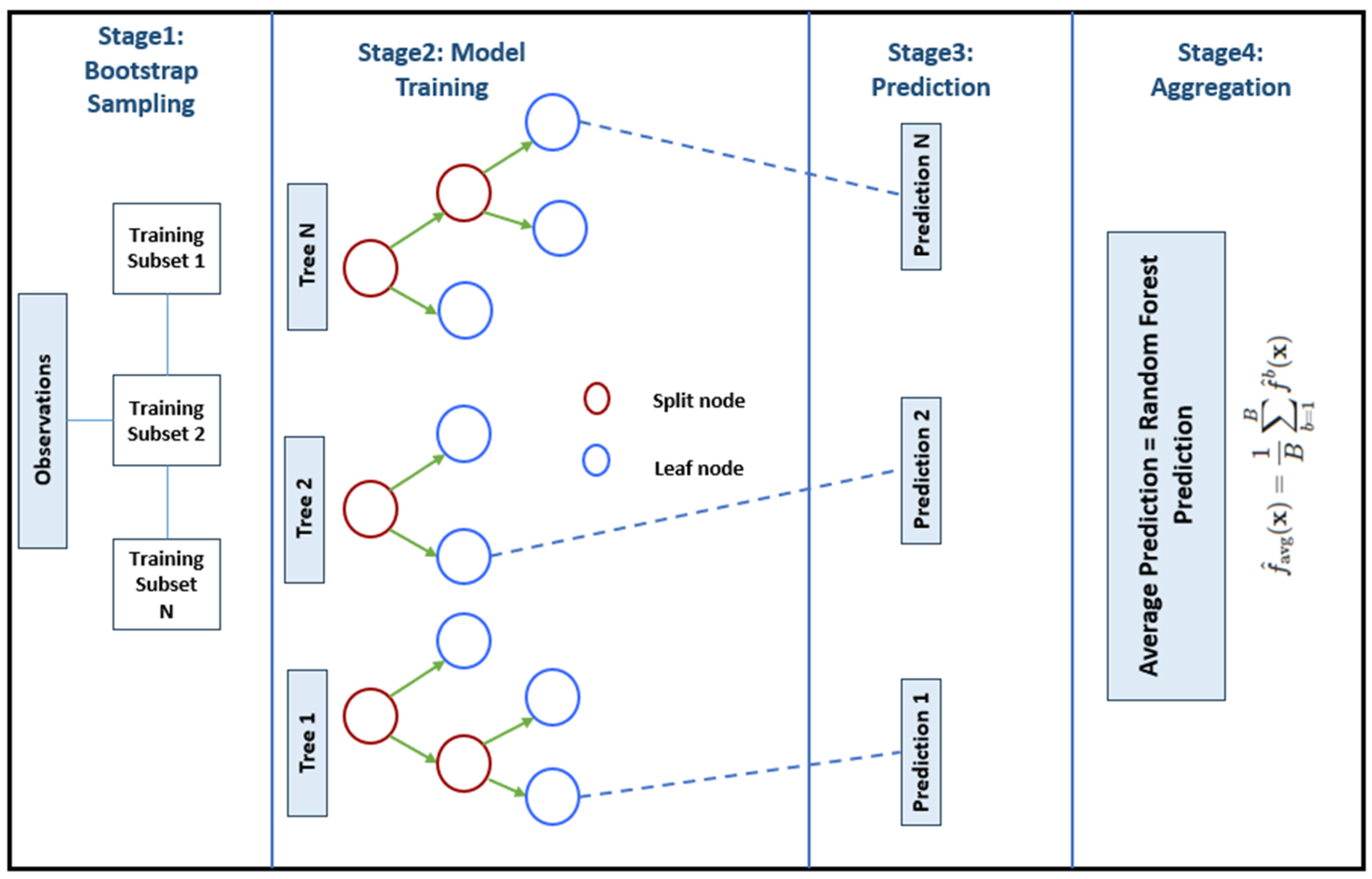
In this study, Random Forest (RF) algorithm was used to predict methane concentrations from the TGS sensor outputs, temperature and relative humidity measured by the DHT22. In RF algorithm, a group decision trees acts as flowcharts where the internal nodes represent decisions made on features and branches representing the decision outcome, and the leaf nodes being the final prediction (Figure 3). The first step in RF is the creation of subsets of the original dataset, where data is drawn with replacement from the original dataset. This approach reduces overfitting by enabling each tree to be created with different subsets of data and minimizes the correlation between the trees without increasing the variance [33]. The second stage randomly selects a subset of features to construct decision trees, and this ensures diverse trees since not all trees make the same splits and prevents similarity between trees. By generating a diverse and uncorrelated group of trees, this process helps to minimize predictive errors, ultimately producing a stronger and more reliable final prediction. To make a prediction, the individual tree outputs are aggregated and hence a prediction is made.
The data from the two methane sensors and the DHT22 were compiled in one file. Since the data was collected synchronously from all sensors, each timestamp corresponded to a complete set of sensor readings, hence eliminating the need for imputation and guaranteed that there were no missing data points. The data gathering script also ensured that all sensor signals were availed before being written to the main file, but introduced few extra seconds delay in cases where the DHT22 sensor signals were not received. This approach guaranteed the completeness of the datasets. With the collocated reference instrument (Aeris MIRA) sampling at a higher frequency than the metal oxide sensor, the Aeris data was averaged to 1s for comparison with the metal oxide sensors’ data. From the merged datafile, 10% of the data was picked at random, without replacement and without repetition, and used to train and test the RF model using the steps highlighted in the model training section.

2.4.2. Model Training

Google Colab environment was employed as the primary environment for training, saving and making predictions using the model. This environment provided an ideal Graphical Processing Unit (GPU) to efficiently handle the dataset and run the Random Forest Regressor model. Within the environment, pandas library was used for data manipulation and analysis, Scikit-Lean library for machine learning tools, Joblib library for object serialization and matplotlib for visualizations. The RF model input data was split into training and testing using 80-20 criteria, and the split was done randomly to eliminate bias and ensure a well representation of the data distribution. The trained random forest regressor model was stored and used to calculate mixing ratios based on the metal oxide and DHT22 temperature and humidity outputs.

2.4.4. Model Evaluation Metrics

Methane mixing ratios calculated using the ML approach were compared to mixing ratios measured by the Aeris Ultra analyzer output using the coefficient of determination (R2) of the linear regression between the data, the mean absolute error (MAE), the mean squared error (MSE), the root mean squared error (RMSE), the mean absolute percentage error (MAPE) and the explained variance score. The feature importance, which is the measure of how each input variable contributes to the model prediction, was also evaluated for the ML calculated data. Feature importance is determined by evaluating the reduction in impurity (measure of how mixed or uncertain the target variable is within a node) at each node, regulated by the probability of reaching that node [35]. The node probability is the number of nodes reaching that node divided by the total number of samples. The higher the value the more important the feature, and higher values indicate greater feature importance. Histograms of measured and modelled mixing ratio data, comprising of 0.2 ppm bins truncated at < 2ppm and >5 ppm, were compared using the overlap coefficient to investigate the overlap of data.

3. Results

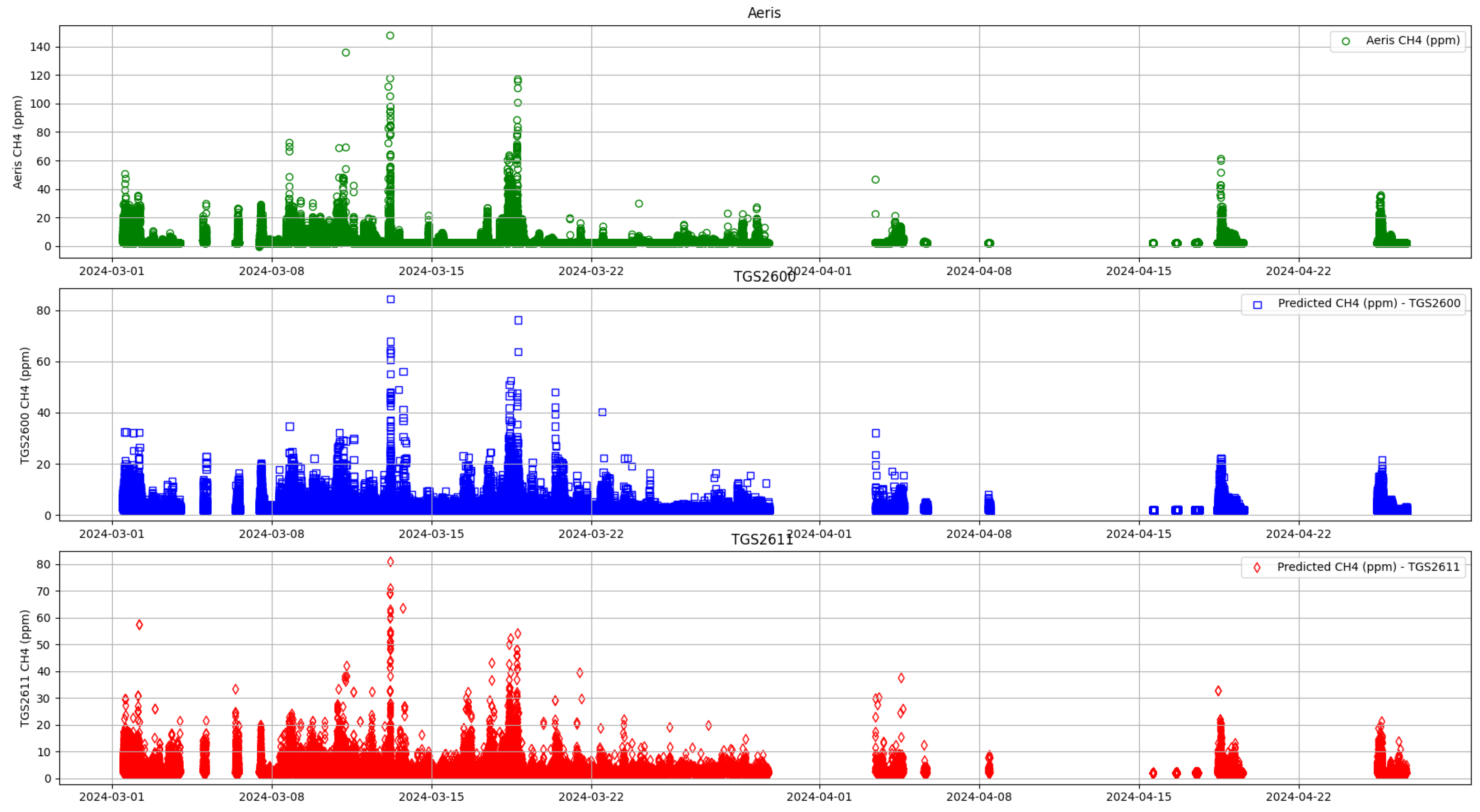
Methane mixing ratios observed by the Aeris Ultra analyzer ranged from background (2ppm) to 147.6 ppm (Figure 4). Throughout the experiment, the temperature varied with large diurnal cycles from a maximum of 27 °C to a minimum of -5 °C with relative humidity cycling similarly between a maximum of 91% and minimum of 18%.

3.1. Eugster and Kling (2012) Calibration Method

3.1.1. Calibration Curves

Previous studies describing the use of metal oxide sensors to measure methane concentrations in air have reported either linear or exponential relationships between (Rs/R0)corr and methane mixing ratios measured by a trace methane analyzer [17,23,24,25,26,30,31,36]. Unlike these studies, the TGS sensors used in this study did not respond in the same way and there was no discernible relationship between (Rs/R0) corr and methane mixing ratio with R2 of 0.0016 and 0.0016 for the TGS2600 and TGS2611, respectively (Figure 5A,B).
It was later discovered that the resistor used to form the Wheatstone bridge with the TGS sensors was 20 times larger than suggested by other studies [25,30] and resulted in a very small signal to noise ratio that had not been observed by the other studies. This meant that the data reported by the TGS sensors used in this study could not be calibrated using the methods described by other papers. When the calibration algorithms were used to calculate the methane mixing ratio and compared against the measurement data for the rest of the campaign (March 12th to May 2nd, 2024) the correlation is zero (Figure 6A,B).

3.2. Machine Learning Methods

A time series plot of the RF predicted methane concentrations showed a similar pattern to the actual measured concentrations from the Aeris analyzer (Figure 4). The model demonstrated a high sensitivity to the minor variations in input features enabling noticeable concentration levels with slight changes in sensor and environmental readings. The average measured concentration for the Aeris analyzer (during the measurement period) was 2.40 ppm with a maximum of 147.6 ppm compared to the average calculated mixing ratios of 2.42 ppm and 2.40 ppm with a maximum value of 105.9 ppm and 106.3 ppm for the TGS2600 and TGS2611, respectively. The gradient of the regression between the measured mixing ratios and those calculated from the TGS2600 data was 0.71 with an R2 of 0.28, while the gradient for the TGS2611 was 0.69 and R2 of 0.25.
The Mean Squared Error values of 2.20 for the TGS2600 and 2.28 for the TGS2611 shows the presence of extensive prediction errors, with RMSE values of 1.48 ppm and 1.51 ppm suggesting that typical concentration prediction errors were around these figures (Table 1). The Mean Absolute Percentage Error suggests that the model’s predictions were, on average, off by approximately 9.66% and 10.76% from the actual values for the TGS2600 and 2611, respectively. Finally, the Explained Variance Scores, indicated that the model accounted for about 28% and 25% of the variance in CH4 concentrations, for TGS2600 and TGS2611 respectively.
The relative contribution of each feature was also assessed and from these, TGS2600 feature importance scores indicate that the relative humidity feature is the most influential, accounting for approximately 35.8% of the model’s predictive power, the sensor resistance at 33.5% and temperature at 30.7%. In the case of the TGS2611, humidity again emerges as the most significant feature, contributing 39.5% to the model’s predictions, while the resistance accounts for 32.1% and temperature contributes 28.4%. The consistent significance of humidity across both sensor models suggests its critical role in the accuracy of sensor measurements.
Histograms, comprising of 17 0.2 ppm bins truncated at < 2ppm and >5 ppm (Figure 7), show all data sets are heavily right skewed. Comparisons using the overlap coefficient, also known as Szymkiewicz-Simpson coefficient, show an overlap between the measured mixing ratios and those mixing ratios generated by TGS2600 and TGS2611 of 0.95 and 0.94, respectively. This means that the measured mixing ratios and mixing ratios generated by TGS2600 has 95% of distribution overlapping whereas with TGS2611, it is 94%.

4. Discussion

This study reports the response of two metal oxide sensors, Figaro TGS2600 and TGS2611, to methane emissions at Colorado State University’s METEC site between March 1st and May 2nd, 2024. Methane mixing ratios observed by the reference analyzer ranged from background to 119 ppm (Figure 5A), while both TGS sensors response showed diurnal variation in response to changes in temperature and relative humidity but no obvious response to changes in methane mixing ratio. When the TGS response data collected during the first two weeks were used to generate calibration curves following published methods [25,30], there was no correlation between the calculated mixing ratios and the measured mixing ratios (Figure 6A,B). A set of training data were then used with the Random Forest machine learning algorithm using the resistance, temperature and relative humidity data to map to the measured reference methane mixing ratio data. These algorithms were then populated with TGS2600 and TGS2611 data from the remainder of the measurement period to calculate methane mixing ratios.

4.1. Random Forest Calibration versus Linear Regression Calibration

The random forest algorithm performed better than the linear regression model. The R2 for the linear regression model for TGS2600 and TGS2611 are 0.002 and 0.002, respectively, compared to the R2 obtained by the RF model, 0.28 and 0.25, respectively (Table 1). This can be attributed to the ability of the RF algorithm to capture non-linear and convoluted interrelations between the sensor outputs and the target variable. In addition, the ability of the RF model to implement bootstrapping and feature randomness reduces the risk of overfitting while allowing the model to popularize better to new datasets.

4.2. Influence of Humidity & Temperature

The signal-to-noise ratio of the metal oxide data was too low for previously used calibration methods to be employed. The sensors were deployed through periods of low and high temperatures and also at high fluctuation in humidity. Therefore, the RF algorithm was able to identify the underlying complex relationship between the sensor resistances and the variable conditions that the sensors were exposed to. Humidity was found to be the most influential factor for both sensors, and this could be as a result of formation of a layer of water molecules on the sensing element altering the sensors response greatly. There might have also been a calibration drift in the sensor due to prolonged exposure to humidity especially in the early stages, and the model weighted the humidity data more heavily on the predictions. The quality of methane mixing ratio data calculated using the machine learning derived algorithms is similar to those reported previously even though there was a much lower signal-to-noise ratio of input data. Eugster and Kling (2012) reported a R2 between modeled and measured data between 1.85 and 1.00 ppm of 0.19 [25], while this study reports an R2 over the same range of mixing ratios of 0.13. Collier-Oxandale et al. (2018) reported an RMSE of 0.38 for mixing ratios between 2 and 7 ppm of 0.38 [37], while this study reports an RMSE of 1.35. Riddick et al. (2020a) reported an accuracy of ± 0.01 ppm between 1.85 and 5.85 ppm while this study reports an accuracy of ± 0.24 ppm.

4.3. Summary

This study provides evidence that machine learning approaches could be used to generate sensor calibration algorithms to better constrain methane mixing ratios measured using low-cost methane sensors. Practically, this would mean that machine learning could be used to derive algorithms to better define complex relationships between sensor outputs and environmental conditions to enable better calibration and improve the metal oxides sensor’s accuracy. The main advantages of using machine learning algorithms for generating calibration algorithms is they can model complex relationships between sensor outputs and environmental conditions, and they reduce the effects of overfitting by using multiple trees. The shortcomings are that with larger datasets, the computational costs increase significantly and that the model interaction between the features are less interpretable as compared to simpler models like linear regression. The development of machine learning algorithms is increasing exponentially, and it is expected that in the future the model can perform better even with less training data while being less affected by noise or sensor anomalies.

5. Conclusions

This study investigated the use of a machine learning model to calibrate poor quality low-cost, metal oxide sensor data to generate representative methane mixing ratio data. Currently, calibration of metal oxide sensors requires a sensor output with a high signal-to-noise ratio. The high importance of humidity in both TGS2600 and TGS2611 sensors underscores the importance of environmental variability when developing predictive models for gas detection.
Our results also showed that the machine learning derived mixing ratios were as good as those reported by other studies using better signal-to-noise ratio data. Here we suggest that, with advances in machine learning, the response of lower-cost sensors could be used to generate mixing ratios with precision and accuracy comparable to higher price trace methane analyzers. This would improve low-cost sensors’ response, give more confidence to calculated emissions and reduce the uncertainty in greenhouse gas emission inventories.

Author Contributions

EK: Conceptualization, Investigation, Methodology, Supervision, Writing – original draft preparation, review and editing. SNR: Funding Acquisition, Conceptualization, Investigation, Methodology, Supervision, Writing – original draft preparation, review and editing. MM: Investigation, Review and Editing. AU: Review and Editing. AA: Review and Editing. DJZ: Funding Acquisition, Project Administration, Conceptualization, Supervision, Review and editing.

Funding

This project has been funded by the U.S. Department of Energy’s Office of Fossil Energy and Carbon Management (FECM) project # DE-FE0032276 “Capabilities Enhancement for Methane Emissions Technology Evaluation Center (METEC) to Decarbonize Natural Gas Resources”.

Institutional Review Board Statement

Not applicable.

Informed Consent Statement

Not applicable.

Data Availability Statement

The original contributions presented in the study are included in the article, further inquiries can be directed to the corresponding author.

Conflicts of Interest

The authors declare no conflicts of interest.

References

  1. IPCC Climate Change 2013 - The Physical Science Basis: Working Group I Contribution to the Fifth Assessment Report of the Intergovernmental Panel on Climate Change; Cambridge University Press: Cambridge, 2014. ISBN 978-1-107-41532-4.
  2. IPCC Climate Change 2022: Impacts, Adaptation and Vulnerability. Contribution of Working Group II to the Sixth Assessment Report of the Intergovernmental Panel on Climate Change [H.-O. Pörtner, D.C. Roberts, M. Tignor, E.S. Poloczanska, K. Mintenbeck, A. Alegría, M. Craig, S. Langsdorf, S. Löschke, V. Möller, A. Okem, B. Rama (Eds.)].; Cambridge University Press.: Cambridge University Press, Cambridge, UK and New York, NY, USA, 2022. ISBN 978-1-00-932584-4.
  3. Global Methane Pledge Global Methane Pledge - Fast Action on Methane to Keep a 1.5°C Future within Reach. Available online: www.globalmethanepledge.org (accessed on 15 September 2022).
  4. UNFCCC Paris Agreement. United Nations Framework Convention on Climate Change. FCCC/CP/2015/L.9/Rev.1. Available online: https://unfccc.int/documents/9064 (accessed on 16 June 2023).
  5. UNEP/CCAC United Nations Environment Programme and Climate and Clean Air Coalition (2021). Global Methane Assessment: Benefits and Costs of Mitigating Methane Emissions. Nairobi: United Nations Environment Programme. Available online: https://www.ccacoalition.org/en/resources/global-methane-assessment-full-report (accessed on 25 October 2022).
  6. Bell, C.; Ilonze, C.; Duggan, A.; Zimmerle, D. Performance of Continuous Emission Monitoring Solutions under a Single-Blind Controlled Testing Protocol. Environ. Sci. Technol. 2023, 57, 5794–5805. [Google Scholar] [CrossRef] [PubMed]
  7. Caulton, D.R.; Lu, J.M.; Lane, H.M.; Buchholz, B.; Fitts, J.P.; Golston, L.M.; Guo, X.; Li, Q.; McSpiritt, J.; Pan, D.; et al. Importance of Superemitter Natural Gas Well Pads in the Marcellus Shale. Environ. Sci. Technol. 2019, 53, 4747–4754. [Google Scholar] [CrossRef] [PubMed]
  8. Riddick, S.N.; Cheptonui, F.; Yuan, K.; Mbua, M.; Day, R.; Vaughn, T.L.; Duggan, A.; Bennett, K.E.; Zimmerle, D.J. Estimating Regional Methane Emission Factors from Energy and Agricultural Sector Sources Using a Portable Measurement System: Case Study of the Denver–Julesburg Basin. Sensors 2022, 22, 7410. [Google Scholar] [CrossRef] [PubMed]
  9. Albertson, John.D.; Harvey, T.; Foderaro, G.; Zhu, P.; Zhou, X.; Ferrari, S.; Amin, M.S.; Modrak, M.; Brantley, H.; Thoma, E.D. A Mobile Sensing Approach for Regional Surveillance of Fugitive Methane Emissions in Oil and Gas Production. Environ. Sci. Technol. 2016, 50, 2487–2497. [CrossRef]
  10. GRI and EPA Harrison, M.R., Shires, T.M., Wessels, J.K., Cowgill, R. M. Methane Emissions from the Natural Gas Industry, Volumes 1 – 15, Final Report, GRI-94/0257 and EPA-600/R-96- 080, Gas Research Institute and US Environmental Protection Agency, June 1996. 1996.
  11. Campbell, L.M.; Campbell, M.V.; Epperson, D.L. Methane Emissions from the Natural Gas Industry, Volume 2: Technical Report, Final Report, GRI-94/0257.1 and EPA-600/R-96-080b. Gas Research Institute and U.S. Environmental Protection Agency. 1996.
  12. Riddick, S.N.; Mauzerall, D.L. Likely Substantial Underestimation of Reported Methane Emissions from United Kingdom Upstream Oil and Gas Activities. Energy Environ. Sci. 2023, 16, 295–304. [Google Scholar] [CrossRef]
  13. Caulton, D.R.; Li, Q.; Bou-Zeid, E.; Fitts, J.P.; Golston, L.M.; Pan, D.; Lu, J.; Lane, H.M.; Buchholz, B.; Guo, X.; et al. Quantifying Uncertainties from Mobile-Laboratory-Derived Emissions of Well Pads Using Inverse Gaussian Methods. Atmospheric Chem. Phys. 2018, 18, 15145–15168. [Google Scholar] [CrossRef]
  14. Peischl, J.; Eilerman, S.J.; Neuman, J.A.; Aikin, K.C.; de Gouw, J.; Gilman, J.B.; Herndon, S.C.; Nadkarni, R.; Trainer, M.; Warneke, C.; et al. Quantifying Methane and Ethane Emissions to the Atmosphere From Central and Western U.S. Oil and Natural Gas Production Regions. J. Geophys. Res. Atmospheres 2018. [CrossRef]
  15. Pétron, G.; Karion, A.; Sweeney, C.; Miller, B.R.; Montzka, S.A.; Frost, G.J.; Trainer, M.; Tans, P.; Andrews, A.; Kofler, J.; et al. A New Look at Methane and Nonmethane Hydrocarbon Emissions from Oil and Natural Gas Operations in the Colorado Denver-Julesburg Basin. J. Geophys. Res. Atmospheres 2014, 119, 6836–6852. [Google Scholar] [CrossRef]
  16. Barkley, Z.; Davis, K.; Miles, N.; Richardson, S.; Deng, A.; Hmiel, B.; Lyon, D.; Lauvaux, T. Quantification of Oil and Gas Methane Emissions in the Delaware and Marcellus Basins Using a Network of Continuous Tower-Based Measurements. Atmospheric Chem. Phys. 2023, 23, 6127–6144. [Google Scholar] [CrossRef]
  17. Riddick, S.N.; Ancona, R.; Cheptonui, F.; Bell, C.S.; Duggan, A.; Bennett, K.E.; Zimmerle, D.J. A Cautionary Report of Calculating Methane Emissions Using Low-Cost Fence-Line Sensors. Elem. Sci. Anthr. 2022, 10, 00021. [Google Scholar] [CrossRef]
  18. Cho, Y.; Smits, K.M.; Riddick, S.N.; Zimmerle, D.J. Calibration and Field Deployment of Low-Cost Sensor Network to Monitor Underground Pipeline Leakage. Sens. Actuators B Chem. 2022, 355, 131276. [Google Scholar] [CrossRef]
  19. Vaughn, T.L.; Bell, C.S.; Pickering, C.K.; Schwietzke, S.; Heath, G.A.; Pétron, G.; Zimmerle, D.J.; Schnell, R.C.; Nummedal, D. Temporal Variability Largely Explains Top-down/Bottom-up Difference in Methane Emission Estimates from a Natural Gas Production Region. Proc. Natl. Acad. Sci. 2018, 115, 11712–11717. [Google Scholar] [CrossRef]
  20. Riddick, S.N.; Mbua, M.; Santos, A.; Hartzell, W.; Zimmerle, D.J. Potential Underestimate in Reported Bottom-up Methane Emissions from Oil and Gas Operations in the Delaware Basin. Atmosphere 2024, 15, 202. [Google Scholar] [CrossRef]
  21. Bell, C.S.; Vaughn, T.L.; Zimmerle, D.; Herndon, S.C.; Yacovitch, T.I.; Heath, G.A.; Pétron, G.; Edie, R.; Field, R.A.; Murphy, S.M.; et al. Comparison of Methane Emission Estimates from Multiple Measurement Techniques at Natural Gas Production Pads. Elem Sci Anth 2017, 5, 79. [Google Scholar] [CrossRef]
  22. Bell, C.; Rutherford, J.; Brandt, A.; Sherwin, E.; Vaughn, T.; Zimmerle, D. Single-Blind Determination of Methane Detection Limits and Quantification Accuracy Using Aircraft-Based LiDAR. Elem. Sci. Anthr. 2022, 10, 00080. [Google Scholar] [CrossRef]
  23. Shah, A.; Laurent, O.; Lienhardt, L.; Broquet, G.; Rivera Martinez, R.; Allegrini, E.; Ciais, P. Characterising the Methane Gas and Environmental Response of the Figaro Taguchi Gas Sensor (TGS) 2611-E00. Atmospheric Meas. Tech. 2023, 16, 3391–3419. [Google Scholar] [CrossRef]
  24. Shah, A.; Laurent, O.; Broquet, G.; Philippon, C.; Kumar, P.; Allegrini, E.; Ciais, P. Determining Methane Mole Fraction at a Landfill Site Using the Figaro Taguchi Gas Sensor 2611-C00 and Wind Direction Measurements. Environ. Sci. Atmospheres 2024, 4, 362–386. [Google Scholar] [CrossRef]
  25. Eugster, W.; Kling, G.W. Performance of a Low-Cost Methane Sensor for Ambient Concentration Measurements in Preliminary Studies. Atmospheric Meas. Tech. 2012, 5, 1925–1934. [Google Scholar] [CrossRef]
  26. Eugster, W.; Laundre, J.; Eugster, J.; Kling, G.W. Long-Term Reliability of the Figaro TGS 2600 Solid-State Methane Sensor under Low-Arctic Conditions at Toolik Lake, Alaska. Atmospheric Meas. Tech. 2020, 13, 2681–2695. [Google Scholar] [CrossRef]
  27. Lin, J.J.Y.; Buehler, C.; Datta, A.; Gentner, D.R.; Koehler, K.; Zamora, M.L. Laboratory and Field Evaluation of a Low-Cost Methane Sensor and Key Environmental Factors for Sensor Calibration. Environ. Sci. Atmospheres 2023, 3, 683–694. [Google Scholar] [CrossRef]
  28. Nagahage, I.S.P.; Nagahage, E.A.A.D.; Fujino, T. Assessment of the Applicability of a Low-Cost Sensor–Based Methane Monitoring System for Continuous Multi-Channel Sampling. Environ. Monit. Assess. 2021, 193, 509. [Google Scholar] [CrossRef]
  29. Sugriwan, I.; Soesanto, O. Development of TGS2611 Methane Sensor and SHT11 Humidity and Temperature Sensor for Measuring Greenhouse Gas on Peatlands in South Kalimantan, Indonesia. J. Phys. Conf. Ser. 2017, 853, 012006. [Google Scholar] [CrossRef]
  30. Riddick, S.N.; Mauzerall, D.L.; Celia, M.; Allen, G.; Pitt, J.; Kang, M.; Riddick, J.C. The Calibration and Deployment of a Low-Cost Methane Sensor. Atmos. Environ. 2020, 230, 117440. [Google Scholar] [CrossRef]
  31. Figaro Production Information. TGS 2611 - for the Detection of Methane. Available online: Https://Www.Figarosensor.Com/Product/Docs/TGS%202611C00(1013).Pdf (accessed on 26 August 2021).
  32. Andrews, B.; Chakrabarti, A.; Dauphin, M.; Speck, A. Application of Machine Learning for Calibrating Gas Sensors for Methane Emissions Monitoring. Sensors 2023, 23, 9898. [Google Scholar] [CrossRef] [PubMed]
  33. Breiman, L. Random Forests. Mach. Learn. 2001, 45, 5–32. [Google Scholar] [CrossRef]
  34. MIRA Mobile Methane/Ethane Analyzers. Aeris Technol.
  35. Ellis, C. Hyperparameter Tuning in Random Forests. Available online: https://crunchingthedata.com/hyperparameter-tuning-in-random-forests/ (accessed on 13 August 2024).
  36. Furuta, D.; Sayahi, T.; Li, J.; Wilson, B.; Presto, A.A.; Li, J. Characterization of Inexpensive Metal Oxide Sensor Performance for Trace Methane Detection. Atmospheric Meas. Tech. 2022, 15, 5117–5128. [Google Scholar] [CrossRef]
  37. Collier-Oxandale, A.; Casey, J.G.; Piedrahita, R.; Ortega, J.; Halliday, H.; Johnston, J.; Hannigan, M.P. Assessing a Low-Cost Methane Sensor Quantification System for Use in Complex Rural and Urban Environments. Atmospheric Meas. Tech. 2018, 11, 3569–3594. [Google Scholar] [CrossRef]
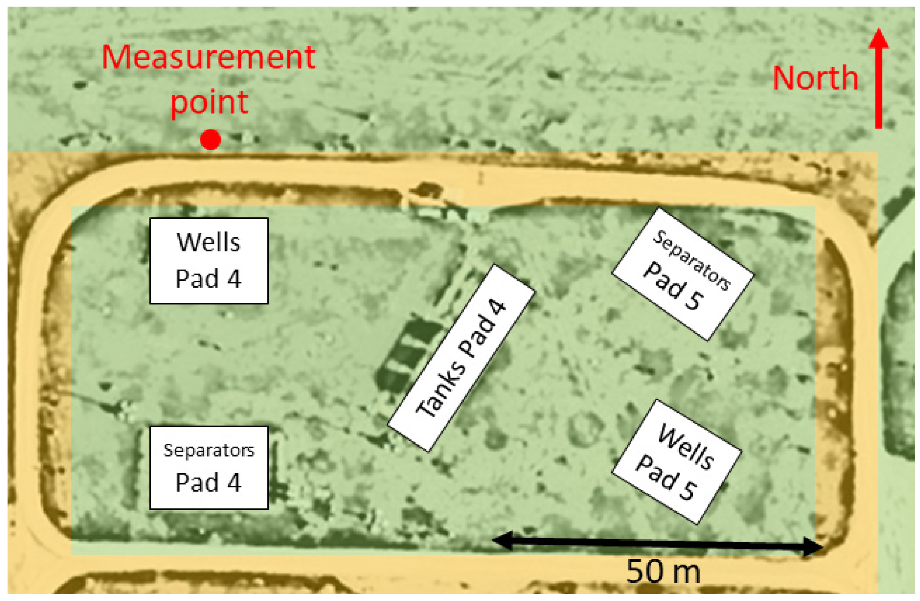
Figure 2. Field layout of the METEC site in Fort Collins with the measurement location on the north of the site.
Preprints 116447 g002
Figure 3. Graphical Representation of Random Forest (RF) regression process.
Preprints 116447 g003
Figure 4. Time series of methane mixing ratios measured by the Aeris Sentinel (top panel), methane mixing ratios calculated using the TGS2600 sensor measurement with a calibration curve generated using machine learning (middle panel) and methane mixing ratios calculated using the TGS2611 sensor measurement with a calibration curve generated using machine learning (bottom panel).
Preprints 116447 g004
Figure 5. Data used to generate a calibration curve following the methods of Eugster and Kling (2012) for the A) TGS2600 and B) the TGS2611. (Rs/R0)corr plotted on the x-axis and methane mixing ratios measured using the Aeris Sentinel on the y-axis.
Preprints 116447 g005
Figure 6. Calculated mixing ratios ([CH4]cal) using the Eugster and Kling (2012) method (y-axis), plotted against methane mixing ratios measured by the Aeris Sentinel (x-axis) for A) the TGS2600 and B) the TGS2611.
Preprints 116447 g006
Figure 7. Histograms, comprising of 15 0.2 ppm bins truncated at < 2ppm and >5 ppm, for the measured mixing ratios (left pane), of the mixing ratios calculated using the TGS2600 data with the RF algorithm (center pane) and mixing ratios calculated using the TGS2611 data with the RF algorithm (right pane).
Preprints 116447 g007
Table 1. Performance metrics for the mixing ratios generated using the TGS2600 data with the RF algorithm (TGS2600-RF) and mixing ratios generated using the TGS2611 data with the RF algorithm (TGS2611-RF) when compared to measured mixing ratios.
Metric TGS2600-RF TGS2611-RF
R-squared (R²) 0.28 0.25
Mean Absolute Error (MAE) 0.33 0.36
Mean Squared Error (MSE) 2.19 2.28
Root Mean Squared Error (RMSE) 1.48 1.51
Mean Absolute Percentage Error (MAPE) 9.66 10.76
Explained Variance Score 0.28 0.25
Disclaimer/Publisher’s Note: The statements, opinions and data contained in all publications are solely those of the individual author(s) and contributor(s) and not of MDPI and/or the editor(s). MDPI and/or the editor(s) disclaim responsibility for any injury to people or property resulting from any ideas, methods, instructions or products referred to in the content.
Copyright: This open access article is published under a Creative Commons CC BY 4.0 license, which permit the free download, distribution, and reuse, provided that the author and preprint are cited in any reuse.
Prerpints.org logo

Preprints.org is a free preprint server supported by MDPI in Basel, Switzerland.

Subscribe

© 2024 MDPI (Basel, Switzerland) unless otherwise stated