1. Introduction
One of the most attractive areas of contemporary probability theory are certainly unit stochastic distributions, defined on the interval
and commonly used as stochastic models that describe so-called proportional (percentage) variables. Thus, they represent theoretical models that can explain the behavior of some real phenomena (see as some more recent ones, e.g., [
1,
2,
3,
4,
5,
6,
7,
8,
9]). Still, it is worth pointing out that modeling with unit distributions is very specific, primarily due to the limitation of the data within the
interval. Although the procedure for creating unit distributions can be given in a rather general form [
10], the most common approach is based on continuous transformations of distributions defined on infinite intervals into a unit interval (see as some recent results, e.g., [
11,
12,
13,
14,
15,
16,
17]). Motivated with procedures similar as in Stojanović et al. [
18,
19], here is presented a novel unit distribution, called the Gumbel–logistic unit (GLU) distribution.
This distribution is based on a general logistic mapping of the Gumbel distribution into a unit interval, which gives it flexibility and convenience for describing various kind of empirical distributions. The definition of the GLU distribution as well as its basic stochastic properties, related to its modality, asymmetry, moments, etc. are described in the next
Section 2. In addition, the hazard rate and quantile functions of the GLU distribution are also discussed in this section. After that,
Section 3 considers the procedure for estimating the parameters of the GLU distribution based on the sample quantiles. The asymptotic properties of thus obtained estimators were also examinated, along with an appropriate Monte Carlo numerical study.
Section 4 presents the application of the GLU distribution in fitting some real–world data, related to telecommunications and machine learning. Finally,
Section 5 provides some concluding highlights.
3. Parameters Estimation & Numerical Simulation Study
In this Section the estimation of the unknown parameters
of the GLU-distributed RV
X is described, based on its observed random sample
of length
n. Let us note first that according to the aforementioned properties of the GLU distribution, some common procedures for estimating its parameters are not appropriate here. For instance, according to Equation (
9), it follows that the moments of the GLU distribution cannot be expressed in a closed form, and thus the method of moments cannot be successfully applied. Similarly, the maximum likelihood (ML) estimation method is also associated with certain difficulties, related to numerically finding solutions
that maximize the likelihood function:
For these reasons, and similar as in Stojanović et al. [
18], Stojanović et al. [
19], here we consider parameter estimation methods based on the quantiles of the GLU distribution. These estimators (we will call them Q-estimators) are explicitly given and also have some convenient asymptotic properties, which will be shown below.
In that aim, for a random sample
of the length
n, let us define the appropriate order statistics
. Then the PDF of the
i-th order statistic
, as is known, can be expressed as follows:
where
. On the other hand, by replacing
in the QF
, given by Equation (
16), the quantile
is obtained. Therefore, the appropriate sample quantile can be obtained according to the equality:
where
is the integer part of
. Thus, sample quantiles are actually the order statistics, so their distribution is determined by Equation (
20).
In order to determine the Q-estimators of the parameters of the GLU-distributed RV
X, notice first that for
is obtained the quantile
. Hence, by equating this quantile with sample one
, the estimator of the shape parameter
is simply obtained as follows:
Furthermore, by substituting
into the QF
, it is obtained the median of the GLU distribution:
Thus, by equating median with the sample one
, and using the estimator
, for the estimator of the scale parameter
one obtains:
In the following, some asymptotic properties of the proposed estimators are examined:
Theorem 6. Statistics are consistent and asymptotic normal (AN) estimators of the true parameters .
Proof. To prove the consistency of the proposed estimators, we apply some general results of sample quantile theory. Let us first note that the CDF
is a differentiable and increasing function on
. Therefore, the quantiles
are uniquely determined by Equation (
16), while the sample quantiles
are uniquely determined by Equation (
21). Now, according to Bahadur’s representation of sample quantiles (see, e.g., Theorem 1 in [
22], or Serfling [
23], pp. 91-92), it follows:
where
is the empirical CDF of the GLU-distributed RV
X. It is well known that for arbitrary
, the empirical CDF
almost surely and uniformly converges to the CDF
, when
. Applying this convergence on Equation (
25), when
, one obtains:
i.e., the sample quantiles are consistent estimators of the theoretical ones. At the same time, the estimators
are continuous functions of the sample quantile
, where
, as well as the sample median
. Thus, applying the continuity property of almost sure convergence (see, e.g., Serfling [
23], p. 24), it follows:
i.e.,
are indeed consistent estimators of
.
We now prove the AN properties of the proposed estimators. To this end, note that under the above assumptions, Equation (
25) implies the following convergence in the distribution:
By using Equation (
26), for the sample quantile
, where
, one obtains:
where, according to Equation (
2) and after some calculations, we get:
Hence, applying the continuity of convergence in the distribution (see, e.g., Serfling [
23], p. 118), for the estimator
, defined by Equation (
22), it is obtained:
where:
In a similar way, the AN property of the estimator
, given by Equation (
24), is proved. To that end, let us first notice that Equation (
26), applying on the sample median
, gives the following convergence:
Here, according to Equations (
23) and (
26), as well as after some computations, it follows:
By applying again the continuity of convergence in distribution, one obtains:
where, according to Equations (
23), (
24) and (
28), it follows:
In this way, the convergences proved in Equations (
27) and (
29) confirm the AN properties of both estimators
and
. □
In the following, a numerical study examing the efficiency of the proposed Q-estimators is presented, based on independent Monte Carlo simulations of samples
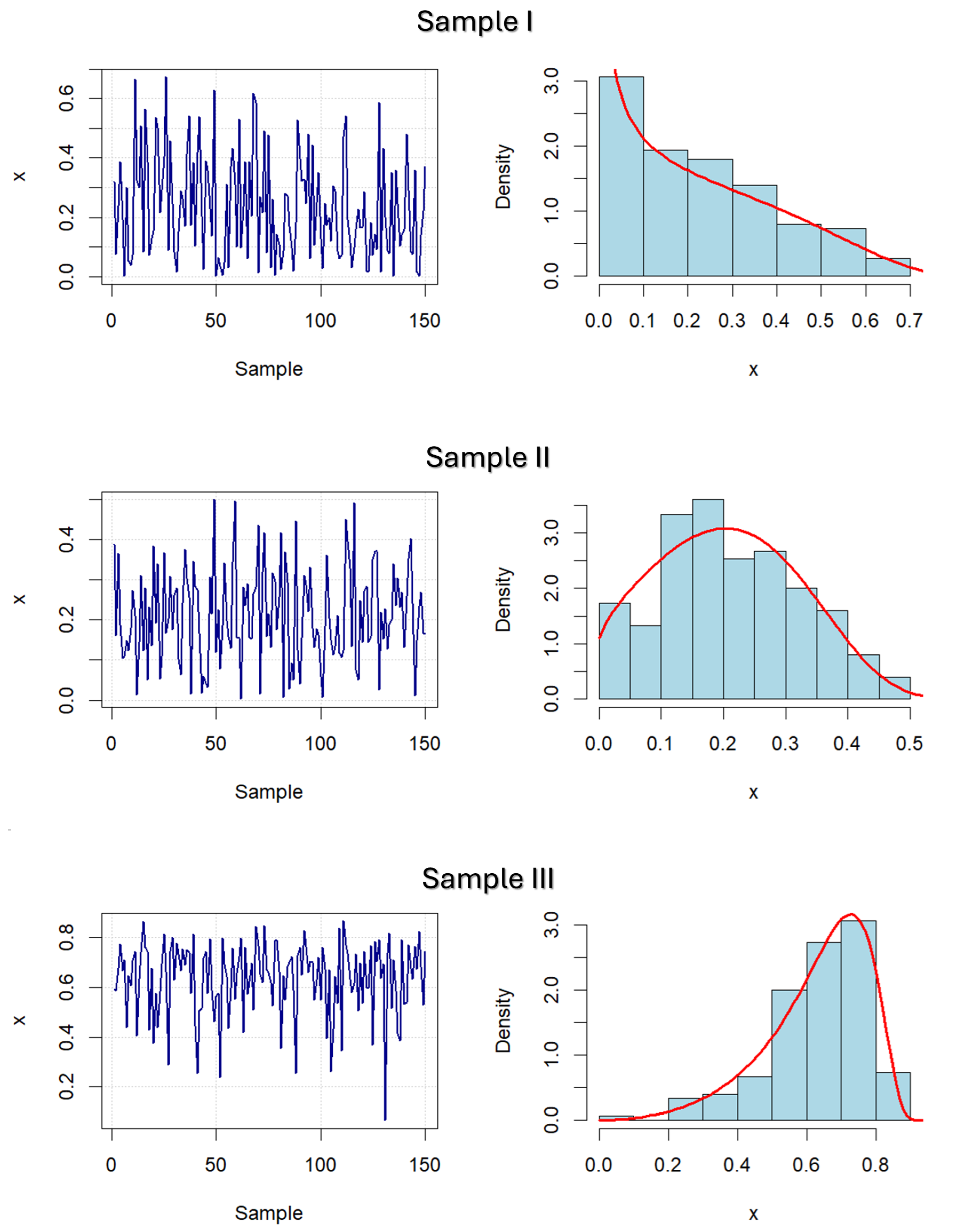
drawn from the GLU distribution. In other words, various samples and parameter values from the GLU distribution were considered, according to which the Q-estimators were calculated, and their statistical analysis was also performed. To that aim, three different samples from the GLU-distribution are examined (also shown in
Figure 5, below):
Sample I is taken from a decreasing GLU distribution, with parameters and , which satisfies the inequality .
Sample II is taken from a unimodal, positively skewed GLU distribution, with parameters and , so the equality holds.
Sample III is taken from a unimodal, negatively skewed GLU distribution, with parameters and , which satisfies the inequality .
Note that the simulated sample values are generated by the R-package "distr" [
24], and thereafter the Q-estimates
and
are calculated using the procedure described above. To additionally check the efficiency of proposed estimators, realizations of samples of different lengths
were considered, so that they are close to the lengths of some of the real-world data that will be analyzed below. In addition, for each of the samples,
independent simulations were conducted, on which an appropriate statistical analysis of the obtained estimates was then performed. The results of this analysis are presented in the following
Table 1,
Table 2 and
Table 3.
More specifically, the above Tables contain summary statistics of the calculated estimates, that is, their minimums (Min.), mean values (Mean) and maximums (Max.). In addition, some error statistics are also shown, i.e., the standard deviations (SD), the mean square errors of estimation (MSEE) and fractional errors of estimation (FEE). Finally, the results of the Anderson-Darling and Shapiro-Wilk normality tests are also given. Based on the results obtained in this way, it can be noted that the proposed estimators are efficient, because the bias, the sample range (Max.–Min.), as well as the values of SD, MSEE and FEE decrease with the increase in the sample size. At the same time, it can be noted that stability and efficiency are more significant at the estimates , especially in the first sample. This obviously follows from the fact that the estimate is calculated by a two-stage procedure, i.e., by using the previously obtained estimate .
Similar conclusions can be made according to the results of AN testing of these estimates. As previously mentioned, AN testing was conducted using Anderson–Darling and Shapiro–Wilk normality tests, whose statistics, labelled by AD and W respectively, as well as the appropriate
p-values were calculated using the R-package "nortest " [
25]. According to the results obtained in this way, also presented in
Table 1,
Table 2 and
Table 3, it can be noted that estimates
have a pronounced AN feature, which applies to all observed samples. On the other hand, estimates
have a less pronounced AN feature, primarily in the case of smaller samples. Nevertheless, the AN property is clearly confirmed in most cases with them as well. Some confirmations of these facts can be also seen in
Figure 5, where the realizations of the samples, as well as their empirical and theoretical distributions, are shown.
4. Applications of the GLU Distribution
As mentioned earlier, the Gumbel distribution can be used to model the extremes of some sample values. In more detail, in his original work Gumbel [
26] has proved that the maximum of a sample taken from a population with an exponential distribution, after a simple transformation, approaches the Gumbel distribution with increasing sample size. This procedure can also be applied in some practical cases, such as in Burke et al. [
27], where the Gumbel distribution is used to analyze maximum rainfall. In a similar way, the maximum load on the telecommunications system, which allows administrators to optimize network capacity and minimize the occurrence of overloads can be modeled with the Gumbel distribution. It is worth pointing that some other application can be in risk analysis related to the ICT technology, which enables companies to better understand and prepare for extreme scenarios that can significantly affect the business by developing methods for the development and introduction of new technologies and concepts, as is shown in Pažun Langović [
28].
For those reasons, this section considers some possible applications of the GLU distribution in real-world data modeling, primarily in the domains of telecommunications and machine learning. The datasets observed here were downloaded from the website “Kaggle.com" [
29], a platform focused on analysing and sharing datasets related to machine learning and online data science. Thereby, the observed data represent parts of the training data related to network and telecommunication traffic in India, i.e., describe the satisfaction and participation of end users, as well as the adaptability and extensibility of the corresponding network transport. More specifically, the three real-world datasets analyzed below can be briefly described as follows:
The first data set, named Series A, consists of
data representing the percentage of service usage time of end users. The data was collected by Mirza [
30] and as already mentioned, it is a part of the training data intended for machine learning and online coding and modeling.
The second one (Series B), are also part of the same training data as above, and consistes of monthly end user fees (in Indian Rupees). In doing so, these data are normalized in relation to their maximum and minimum values, and in this way a set of data in a unit interval is obtained.
Finally, the third set of data, designated as Series C, is obtained from training data authored by Mnassri [
31], intended for the development of appropriate predictive models, i.e., training, cross-validation and performance testing of machine learning models. Therefore, Series C consists of
data, which represent the total daily call length of end users (expressed in minutes), whereby the normalized values are obtained as the ratio of the call duration to the maximum call length.
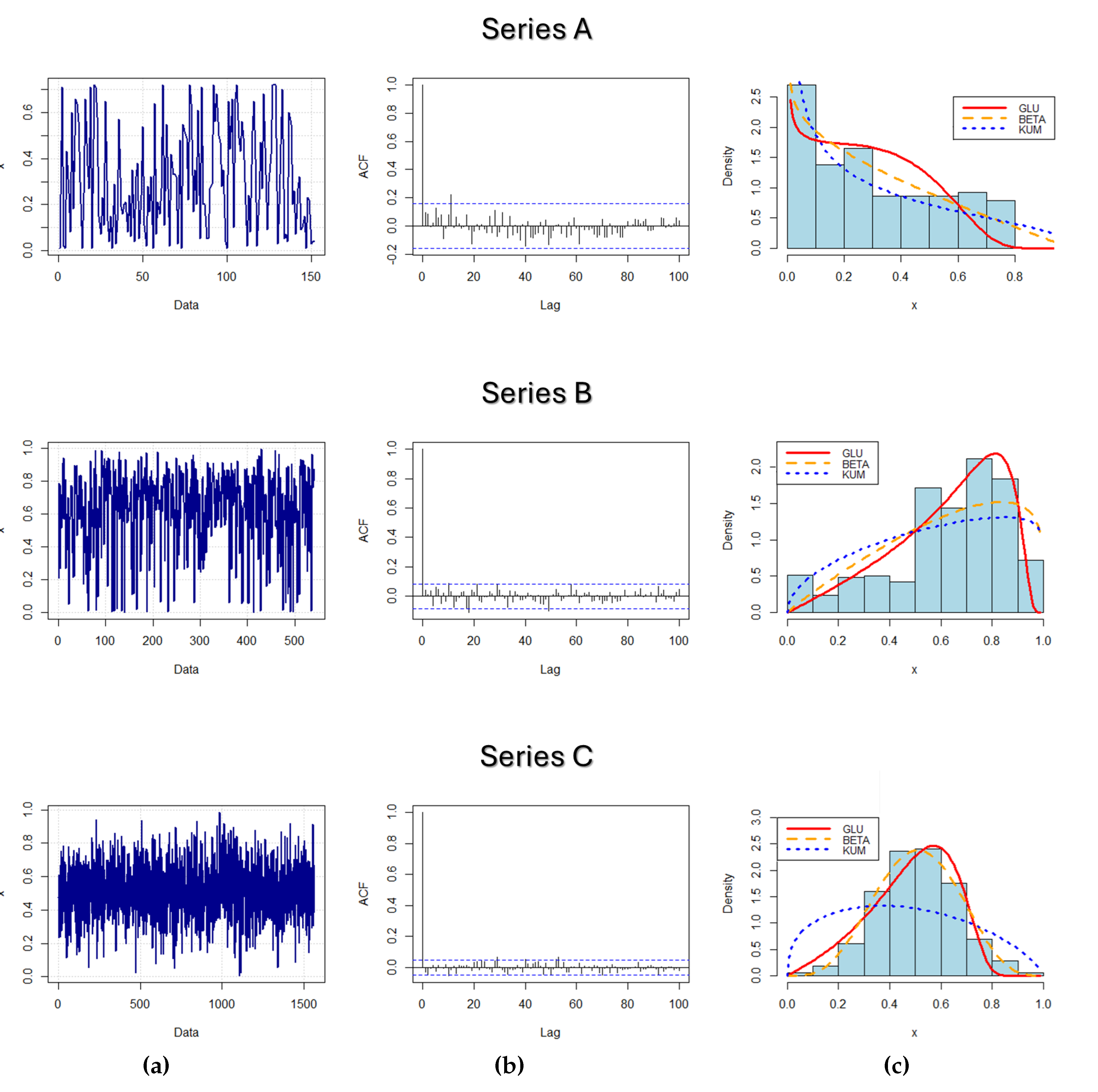
Realizations of these series are shown in
Figure 6(a), while
Figure 6(b) shows the values of their corresponding autocorrelation functions (ACFs). As can be easily seen, the ACF values of all series are realatively low, so they can be considered as independent realizations of some unit RV, that is, they can obviously be modeled by one of the unit stochastic distributions.
In order to additionally verify the effectiveness of such modeling, in addition to the proposed GLU distribution, some other existing, well-known unit distributions were used to fit the empirical distributions of observed data. In more detail, the GLU distribution is compared with two well-known unit distributions, namely the Beta and Kumaraswamy distributions. Their PDFs are, respectively,
where
, as
are distribution parameters, and
is the beta function. To obtain the estimated parameter values of the Beta distribution, the method of moments (MM) is used here (see, e.g., [
32]). According to this, the MM estimates are as follows:
where
and
are the sample mean and variance, respectively, and the inequality
holds. On the other hand, the maximum likelihood (ML) estimation method is used for the Kumaraswamy distribution, according to which estimators are obtained as solutions of coupled equations (see, e.g., Dey et al. [
33]):
As is known, the proposed estimators for both of the above distributions have the properties of stability and asymptotic normality. In this way, one of the reasons for choosing them is the comparison not only with respect to their distribution, but also with respect to different estimation procedures.
The results of the previously described estimation procedures can be seen in
Figure 6(c), where the empirical distributions of the observed data (given by histograms) are shown, along with the corresponding fitted PDFs. As can be easily seen, the empirical distribution of Series A is significantly positively skewed and it is fitted with decreasing theoretical PDFs. On the other side, Series B and Series C have negatively skewed unimodal distributions, with the distribution of Series C being "approximately symmetric" to some extent. This can also be confirmed by the estimated parameter values for each series and for all competing models, which are shown in
Table 4 below.
Based on them,
independent Monte Carlo simulations of the corresponding theoretical distributions were performed and the agreement between the empirical and fitted distributions was checked in several different ways. Namely, the mean square estimation error (MSEE) statistics, the Akaike information criterion (AIC), as well as the Bayesian information criterion (BIC) for model selection were used for this purpose. In addition, the Kolmogorov–Smirnov (KS) test of equivalence of the asymptotic distribution of the two samples was also performed, and all these values are also shown in
Table 4.
According to the results obtained in this way, it is noticeable, for instance, that in the case of Series A all three theoretical distributions can be adequate for fitting. On the contrary, for the other two series, the values of MSEE, AIC and BIC are generally lower in cases where GLU and Beta distribution are applied as appropriate fitting models. Nevertheless, it is clear that the GLU distribution has better fitting characteristics than both other theoretical distributions, even in the case of Series C, which has an "approximately symmetric" distribution. Moreover, only with the GLU distribution, the KS test statistics do not reject, with a significant level , the hypothesis of the equivalence of the theoretical and the observed empirical distribution.
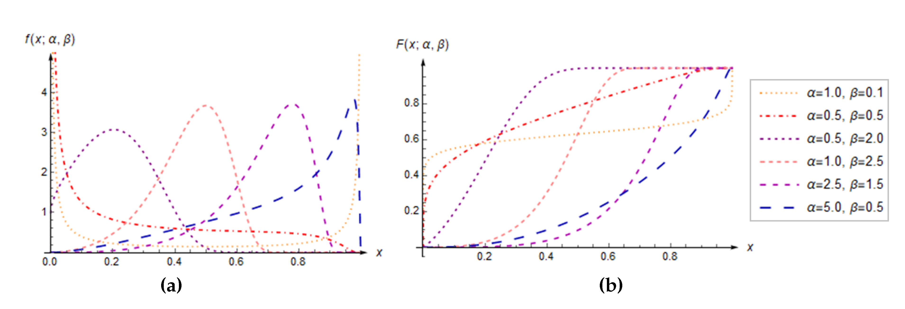
Figure 1.
Plots of the PDFs (a) and CDFs (b) of the GLU distribution for different values of parameters .
Figure 1.
Plots of the PDFs (a) and CDFs (b) of the GLU distribution for different values of parameters .
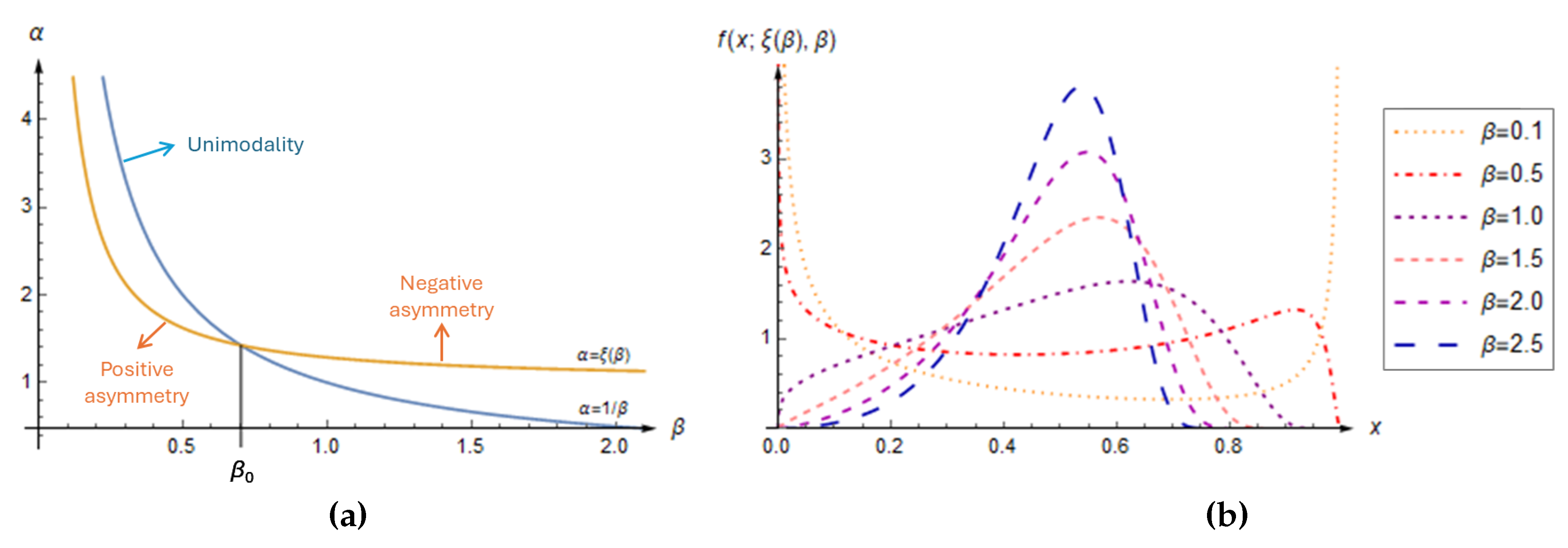
Figure 2.
(a) Parameter areas with different shapes and asymmetry of the GLU distribution. (b) Some PDFs of the GLU distributed RV X, where the dependence holds.
Figure 2.
(a) Parameter areas with different shapes and asymmetry of the GLU distribution. (b) Some PDFs of the GLU distributed RV X, where the dependence holds.
Figure 3.
Plots of the HRF (a) and QF (b) of the GLU distribution, obtained for some parameters values .
Figure 3.
Plots of the HRF (a) and QF (b) of the GLU distribution, obtained for some parameters values .
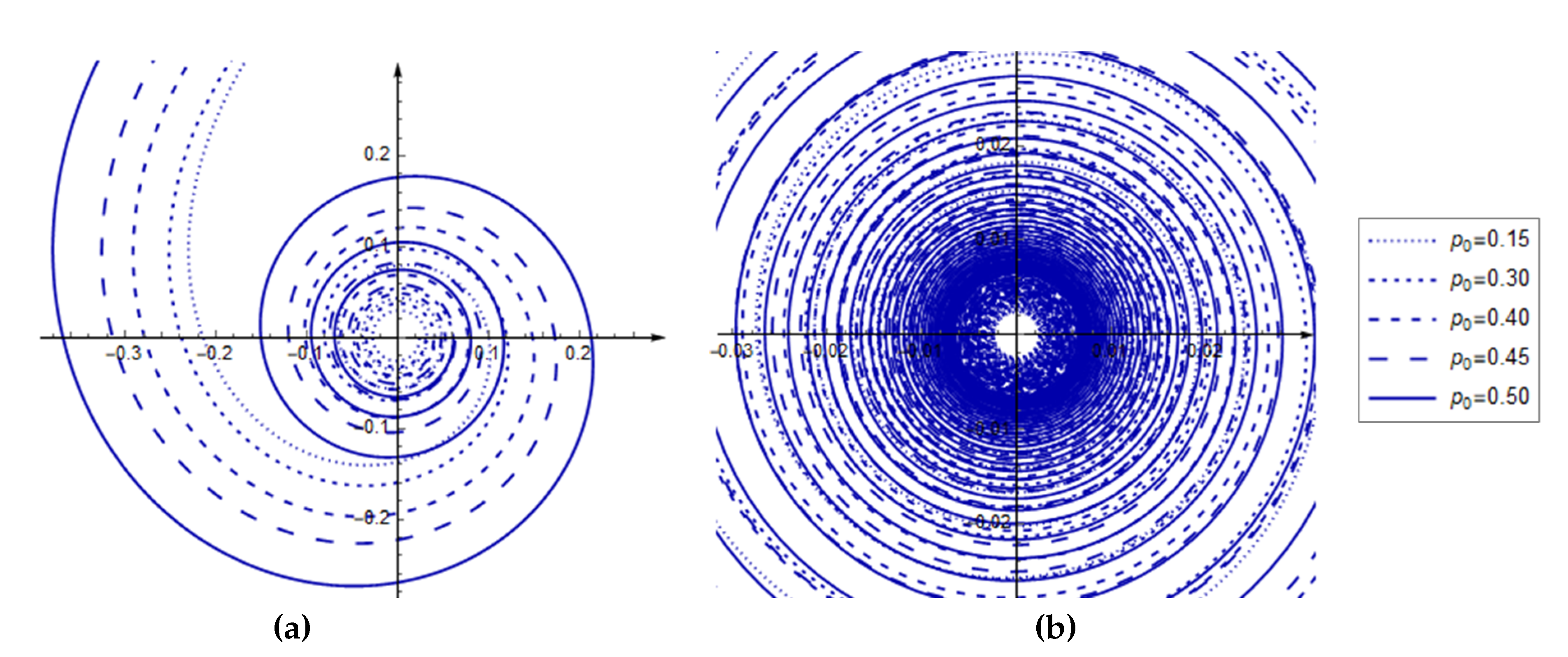
Figure 4.
Polar plots of parameter dependences yielding a unimodal GLU distribution, with some fixed values of and two different angular intervals: (a); (b).
Figure 4.
Polar plots of parameter dependences yielding a unimodal GLU distribution, with some fixed values of and two different angular intervals: (a); (b).
Figure 5.
Left plots: Observations of various samples drawn from the GLU-distribution. Right plots: Empirical and fitted PDFs of the RV .
Figure 5.
Left plots: Observations of various samples drawn from the GLU-distribution. Right plots: Empirical and fitted PDFs of the RV .
Figure 6.
(a): Observed sample values of three real-world data. (b): Estimated ACFs of observed samples (data series). (c): Empirical and fitted PDFs, obtained using the GLU, Beta and Kumaraswamy distributions.
Figure 6.
(a): Observed sample values of three real-world data. (b): Estimated ACFs of observed samples (data series). (c): Empirical and fitted PDFs, obtained using the GLU, Beta and Kumaraswamy distributions.
Table 1.
Summary statistics, estimation errors, and AN testing of parameter estimates of the GLU distribution: Sample I with the true parameter values and .
Table 1.
Summary statistics, estimation errors, and AN testing of parameter estimates of the GLU distribution: Sample I with the true parameter values and .
| Statistics |
|
|
|
|
|
|
|
|
|
| Min. |
0.4015 |
0.5716 |
0.4237 |
0.6739 |
0.4660 |
0.8195 |
| Mean |
0.5122 |
1.1906 |
0.5111 |
1.1519 |
0.5020 |
1.0488 |
| Max. |
0.6101 |
1.8720 |
0.5807 |
1.7959 |
0.5515 |
1.2252 |
| SD |
0.0388 |
0.9769 |
0.0221 |
0.2341 |
0.0122 |
0.0439 |
| MSEE |
0.0403 |
0.3218 |
0.0252 |
0.1906 |
0.0168 |
0.0519 |
| FEE (%) |
8.0623 |
32.177 |
5.0333 |
19.062 |
3.3707 |
5.1930 |
|
0.2933 |
0.5094 |
0.3035 |
0.6068 |
0.2930 |
0.4860 |
| (p-value) |
(0.5997) |
(0.1962) |
(0.5704) |
(0.1137) |
(0.6004) |
(0.2240) |
| W |
0.9929 |
0.9876 * |
0.9946 |
0.9884 * |
0.9957 |
0.9902 |
| (p-value) |
(0.2815) |
(0.0299) |
(0.5138) |
(0.0414) |
(0.7109) |
(0.0890) |
Table 2.
Summary statistics, estimation errors, and AN testing of parameters estimates of the GLU distribution: Sample II with the true parameter values and .
Table 2.
Summary statistics, estimation errors, and AN testing of parameters estimates of the GLU distribution: Sample II with the true parameter values and .
| Statistics |
|
|
|
|
|
|
|
|
|
| Min. |
0.4299 |
1.2050 |
0.4731 |
1.3330 |
0.4821 |
1.5590 |
| Mean |
0.4993 |
2.1085 |
0.4995 |
2.0420 |
0.5000 |
2.0206 |
| Max. |
0.5615 |
2.6790 |
0.5194 |
2.2570 |
0.5155 |
2.1400 |
| SD |
0.0212 |
1.0480 |
9.26
|
0.3665 |
5.58
|
0.2013 |
| MSEE |
0.0181 |
0.3746 |
0.0105 |
0.0862 |
6.22
|
0.0356 |
| FEE (%) |
3.6132 |
18.728 |
2.0931 |
4.3068 |
1.2481 |
1.7883 |
|
0.3802 |
1.0201
|
0.2678 |
0.4337 |
0.2090 |
0.3384 |
| (p-value) |
(0.4005) |
(0.0108) |
(0.6826) |
(0.2998) |
(0.8621) |
(0.5021) |
| W |
0.9914 |
0.9888
|
0.9939 |
0.9900 |
0.9956 |
0.99031 |
| (p-value) |
(0.1504) |
(0.0489) |
(0.4049) |
(0.0834) |
(0.7032) |
(0.0949) |
Table 3.
Summary statistics, estimation errors, and AN testing of parameters estimates of the GLU distribution: Sample III with the parameter values and .
Table 3.
Summary statistics, estimation errors, and AN testing of parameters estimates of the GLU distribution: Sample III with the parameter values and .
| Statistics |
|
|
|
|
|
|
|
|
|
| Min. |
1.6710 |
1.0773 |
1.8330 |
1.1057 |
1.8621 |
1.1950 |
| Mean |
1.9952 |
1.4901 |
1.9978 |
1.5052 |
2.0010 |
1.4970 |
| Max. |
2.2941 |
1.9122 |
2.1605 |
1.7935 |
2.1072 |
1.7245 |
| SD |
0.0949 |
0.6647 |
0.0606 |
0.2910 |
0.0326 |
0.1534 |
| MSEE |
0.0949 |
0.1901 |
0.0523 |
0.0796 |
0.0327 |
0.0482 |
| FEE (%) |
4.7450 |
12.675 |
2.6488 |
5.3096 |
1.6375 |
3.2158 |
|
0.3238 |
2.0687
|
0.2153 |
0.5059 |
0.3041 |
0.5160 |
| (p-value) |
(0.5235) |
(2.83 ) |
(0.8460) |
(0.2001) |
(0.5686) |
(0.1889) |
| W |
0.99376 |
0.9806
|
0.9950 |
0.9903 |
0.9952 |
0.9908 |
| (p-value) |
(0.3865) |
(1.74 ) |
(0.5840) |
(0.0949) |
(0.6194) |
(0.1189) |
Table 4.
Estimated parameters of the LLU, beta, and Kumaraswamy distributions, along with the corresponding estimation errors and fit statistics.
Table 4.
Estimated parameters of the LLU, beta, and Kumaraswamy distributions, along with the corresponding estimation errors and fit statistics.
| Parameter/ |
Series A |
Series B |
Series C |
| Statistic |
GLU |
BETA |
KUM |
GLU |
BETA |
KUM |
GLU |
BETA |
KUM |
|
0.6603 |
0.8939 |
0.5989 |
2.3400 |
1.9597 |
1.5018 |
1.2055 |
4.7587 |
1.3589 |
|
1.1541 |
1.9902 |
1.3840 |
0.8773 |
1.1883 |
1.0948 |
1.5639 |
4.6025 |
1.7445 |
| MSEE |
0.0118 |
0.0153 |
0.0215 |
5.54
|
7.98
|
0.0426 |
2.86
|
3.15
|
0.0573 |
| AIC |
−116.0 |
−69.18 |
−83.81 |
−310.9 |
−145.5 |
−65.37 |
−1423.5 |
−1419.7 |
−218.0 |
| BIC |
−110.0 |
−63.13 |
−77.76 |
−294.3 |
−128.9 |
−48.78 |
−1404.8 |
−1401.0 |
−199.3 |
|
0.0921 |
0.0987 |
0.1316 |
0.0623 |
0.0886
|
0.1495
|
0.0392 |
0.0403 |
0.2398
|
| (p-value) |
(0.5393) |
(0.4498) |
(0.1439) |
(0.1654) |
(0.0285) |
(1.11 ) |
(0.1858) |
(0.1580) |
(0.00) |
