Development of a Three-Dimensional Inversion Program for Magnetotellurics Using Finite Volume and Adjoint State Method

Introduction

Method

Forward Modelling

In general, the MT analysis combines Maxwell’s equations in the frequency domain to form an equation of only the electric or magnetic field, which is then discretized and solved to obtain the electric or magnetic field.

Some discretization methods exist including the finite difference method (FDM) (e.g., Kelbert et al., 2014; Sasaki, 2004; Siripunvaraporn et al., 2005), FEM (e.g., Mitsuhata & Uchida, 2004; Usui, 2015; Usui et al., 2024; Zhu et al., 2022) and FVM (e.g., Jahandari & Farquharson, 2015).

This program adopts the hexahedral cell-centered finite volume method as the forward modeling. The advantages of this method are

1)

the unknowns are placed at the cell center and discretized on the cell surface using a simple method similar to FDM.

2)

Unstructured meshes can be applied as FEM, allowing calculations with topography and local subdivision.

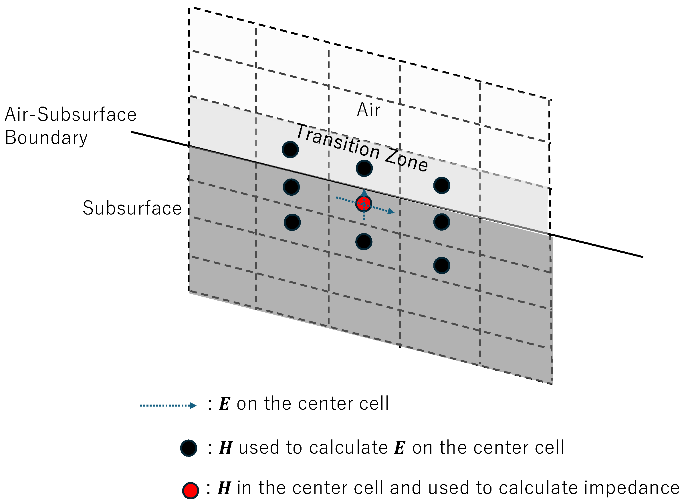
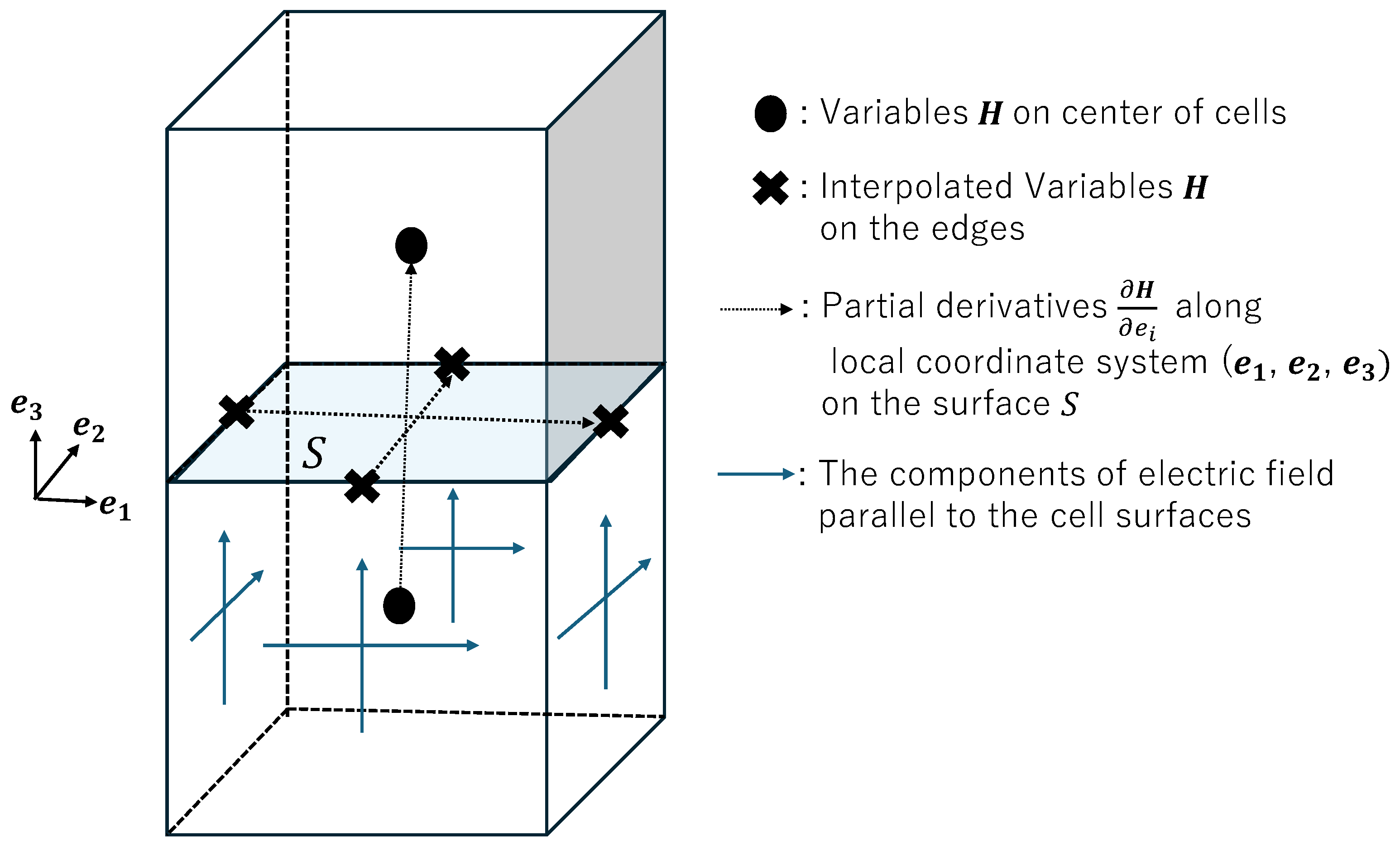
In MT forward modeling, the second-order Maxwell’s equations in the form of the electric $\mathit{E}$ or the magnetic $\mathit{H}$ fields are often solved(Siripunvaraporn, Egbert, and Lenbury 2002). The H-forming equation (1) is solved in this program (Figure 1).

$$\nabla \times \rho \nabla \times \mathit{H}=-i\omega {\mu }_0\mathit{H},$$

(1)

where ω is the angular frequency, μ₀ is the magnetic permeability of the vacuum, and ρ is specific resistance. In FVM, (1) is discretized after volume integration of both sides of Eq. (1), and the left-hand side is converted to surface integration by integral formula.

$$\sum \mathit{n}\times \rho \left(\nabla \times \mathit{H}\right)∆S=-i\omega {\mu }_0\mathit{H}∆V,$$

(2)

where n is the normal vector of each cell surface, ∆S is the Area of each cell surface, ∆and V is the Cell volume. Note that (2) is valid with arbitrary geometry; therefore, if we can properly approximate ∇ × H term on each cell surface, it is possible to use unstructured meshes and local mesh refinement as FEM in Usui et al. (2024). For the air layer, (2) should be modified because of poor convergence. They can be achieved by converting and discretizing (1), assuming $\rho$ is constant in the air layer, and applying the condition ∇ ∙ H = 0 as follows:

$$\sum \mathit{n}·\nabla \mathit{H}∆S= -i\omega {\mu }_0\sigma \mathit{H}∆V,$$

(3)

where $\sigma =1/\rho .$ (3) is a general Poisson equation, which should contribute to the computational stability in the air layer. This program solves (2) and (3) in the subsurface and the air layers, respectively. In (2), ρ on the cell surfaces are needed. This program uses the average as Taylor and Weaver (1976) and Mackie and Madden (1993). For computational stability, a transition layer is provided between the air and subsurface. In this layer, the air resistivity is 10⁶ Ω ∙ m on the surfaces between the air and subsurface (Figure 2).

Figure 1. Schematic cartoon that indicates how to calculate ∂H/∂e_i on the surfaces of cells and the locations of electric field. ${\mathit{e}}_1$and ${\mathit{e}}_2$ are parallel to the surface $\mathit{S}$. Note that this calculation can be applied to not only the structured grid but also the unstructured and non-conforming grid.

Figure 1. Schematic cartoon that indicates how to calculate ∂H/∂e_i on the surfaces of cells and the locations of electric field. ${\mathit{e}}_1$and ${\mathit{e}}_2$ are parallel to the surface $\mathit{S}$. Note that this calculation can be applied to not only the structured grid but also the unstructured and non-conforming grid.

Figure 2. Schematic cartoon of a 2D case that indicates where electromagnetic fields are calculated. H denotes magnetic field.

Figure 2. Schematic cartoon of a 2D case that indicates where electromagnetic fields are calculated. H denotes magnetic field.

To discretize $\nabla \mathit{H}$ in the air layer and ∇ × H in the subsurface layer, ∂H⁄∂x_i on the cell surfaces, where i is 1, 2, or 3 and x_i is a global coordinate system, should be calculated. This can be done by converting the spatial partial differentiation from the local coordinate system (e₁, e₂, e₃) to the global coordinate system, as follows:

$$\left(\begin{array}{c}{\displaystyle \frac{\partial \mathit{H}}{\partial x_1}}\\ {\displaystyle \frac{\partial \mathit{H}}{\partial x_2}}\\ {\displaystyle \frac{\partial \mathit{H}}{\partial x_3}}\end{array}\right)={\left(\begin{array}{ccc}{\mathit{e}}_1·{\mathit{e}}_{{\mathit{x}}_1}& {\mathit{e}}_1·{\mathit{e}}_{{\mathit{x}}_2}& {\mathit{e}}_1·{\mathit{e}}_{{\mathit{x}}_3}\\ {\mathit{e}}_2·{\mathit{e}}_{{\mathit{x}}_1}& {\mathit{e}}_2·{\mathit{e}}_{{\mathit{x}}_2}& {\mathit{e}}_2·{\mathit{e}}_{{\mathit{x}}_3}\\ {\mathit{e}}_3·{\mathit{e}}_{{\mathit{x}}_1}& {\mathit{e}}_3·{\mathit{e}}_{{\mathit{x}}_2}& {\mathit{e}}_3·{\mathit{e}}_{{\mathit{x}}_3}\end{array}\right)}^{-1}\left(\begin{array}{c}{\displaystyle \frac{\partial \mathit{H}}{\partial e_1}}\\ {\displaystyle \frac{\partial \mathit{H}}{\partial e_2}}\\ {\displaystyle \frac{\partial \mathit{H}}{\partial e_3}}\end{array}\right)$$

(4)

${\displaystyle \frac{\partial \mathit{H}}{\partial e_i}}$ (i = 1,2,3) were obtained by interpolation from the surrounding cells.

Boundary conditions on XZ and YZ planes are $\partial \mathit{H}/\partial \mathit{n}$, where $\mathit{n}$is the normal vector. On XY of the subsurface side, $\mathit{H}=0$ is adopted. On XY of the air layer side, the boundary conditions are source terms of the modeling. The author set $H_x$ = 1 and $H_y$ = 1 in twice forward modeling to obtain response functions, respectively (e.g., Siripunvaraporn et al., 2002).

Through these operations, (2) and (3) are discretized, and the linear equation Ax = b (A: coefficient matrix, x: unknown magnetic field vector, b: source term) can be assembled. We can obtain H by solving this equation.

To solve the linear equation, this program adopts BiCGSafe (Fujiwara, Yoshida, and Fujino 2006) with block incomplete LU decomposition as a preconditioner asToh et al. (2000). We set the convergence condition using the maximum change of the solution from the previous iteration ∆$∆{\mathit{x}}_{\mathit{i}}^{\mathit{m}\mathit{a}\mathit{x}}=\max \left({\mathit{x}}_{\mathit{i}}-{\mathit{x}}_{\mathit{i}-1}\right)$, where i is iteration number and the residual ${\mathit{r}}_{\mathit{i}}=A{\mathit{x}}_{\mathit{i}}-\mathit{b}$.

$$\min \left({\displaystyle \frac{\left|r_i\right|}{\left|r_0\right|}},{\displaystyle \frac{\left|∆{\mathit{x}}_{\mathit{i}}^{\mathit{m}\mathit{a}\mathit{x}}\right|}{\left|{\mathit{x}}_{\mathit{i}}^{\mathit{m}\mathit{a}\mathit{x}}\right|}}\right)<ϵ,$$

(5)

where $ϵ$is tolerance.

The divergence correction for subsurface layers is applied as Dong and Egbert (2019), adding a term λ∇(∇ ∙ H), where λ is the scaling factor, to equation (1). In this program, λ is set to ρ × min(1, kω), where k is the safety factor equal to 0.1 because the large value of λ resulted in poor accuracy solutions, especially in long periods.

Once magnetic field H is obtained, the electric field E is necessary at the cell center to calculate the impedance tensor. The following equation is used for this calculation.

$$\mathit{E}=\rho \left(\nabla \times \mathit{H}\right)$$

(6)

Based on equation (6), the electric fields of two directions parallel to cell surfaces are calculated on each cell surface (Figure 1).

$${\mathit{E}}^{center}·{\mathit{p}}_{\mathit{i}\mathit{j}}={\mathit{E}}_{\mathit{i}\mathit{j}}^{\mathit{p}\mathit{a}\mathit{r}\mathit{a}\mathit{l}\mathit{l}\mathit{e}\mathit{l}},$$

(7)

where ${\mathit{E}}^{center}$ is the required electric field at the cell center, ${\mathit{E}}^{\mathit{p}\mathit{a}\mathit{r}\mathit{a}\mathit{l}\mathit{l}\mathit{e}\mathit{l}}$ is the electric field on the cell surface calculated from equation (6), $\mathit{p}$ is the unit vector parallel to the cell surface, $i$ is unit vector directions (1 or 2), and $j$ is cell surfaces number (from 1 to 4). The component of the electric field orthogonal to cell surfaces is excluded because it is not continuous on cell surfaces. From equation (7), eight equations associated with ${\mathit{E}}^{center}$ in each cell can be obtained. Therefore, ${\mathit{E}}^{center}$ can be calculated using the least squares method Because ${\mathit{E}}^{center}$ has three components. Using H and ${\mathit{E}}^{center},$The impedance tensor and magnetic transfer function can be obtained in the same way as in Usui (2015).

Since this program uses the cell-centered FVM, it is necessary to use the surrounding cell-centered magnetic field to obtain the electric field at the cell surface. This program calculates the impedance tensor and magnetic transfer function on the earth’s surface using the electromagnetic fields in the transition zone and near-surface cells, as shown in Figure 2, which is a 2D case.

For the calculation of an impedance tensor with distortion, the method adopted by Ogawa (2002) is used.

$$Z_{calc}=DZ,$$

(8)

where $Z_{calc}$ is the calculated impedance tensor affected distortion, D is the distortion tensor, and Z is the originally calculated impedance tensor.

Note that C++ language is used to implement this program, and the library Eigen (Jacobi, Guennebaud, and other contributor 2024) is used for the internal matrix operations. Parallelization is implemented by OpenMP. The linear equations Ax = b at each frequency are solved on each thread.

Numerical Examples

Forward Modelling Considering Topography.

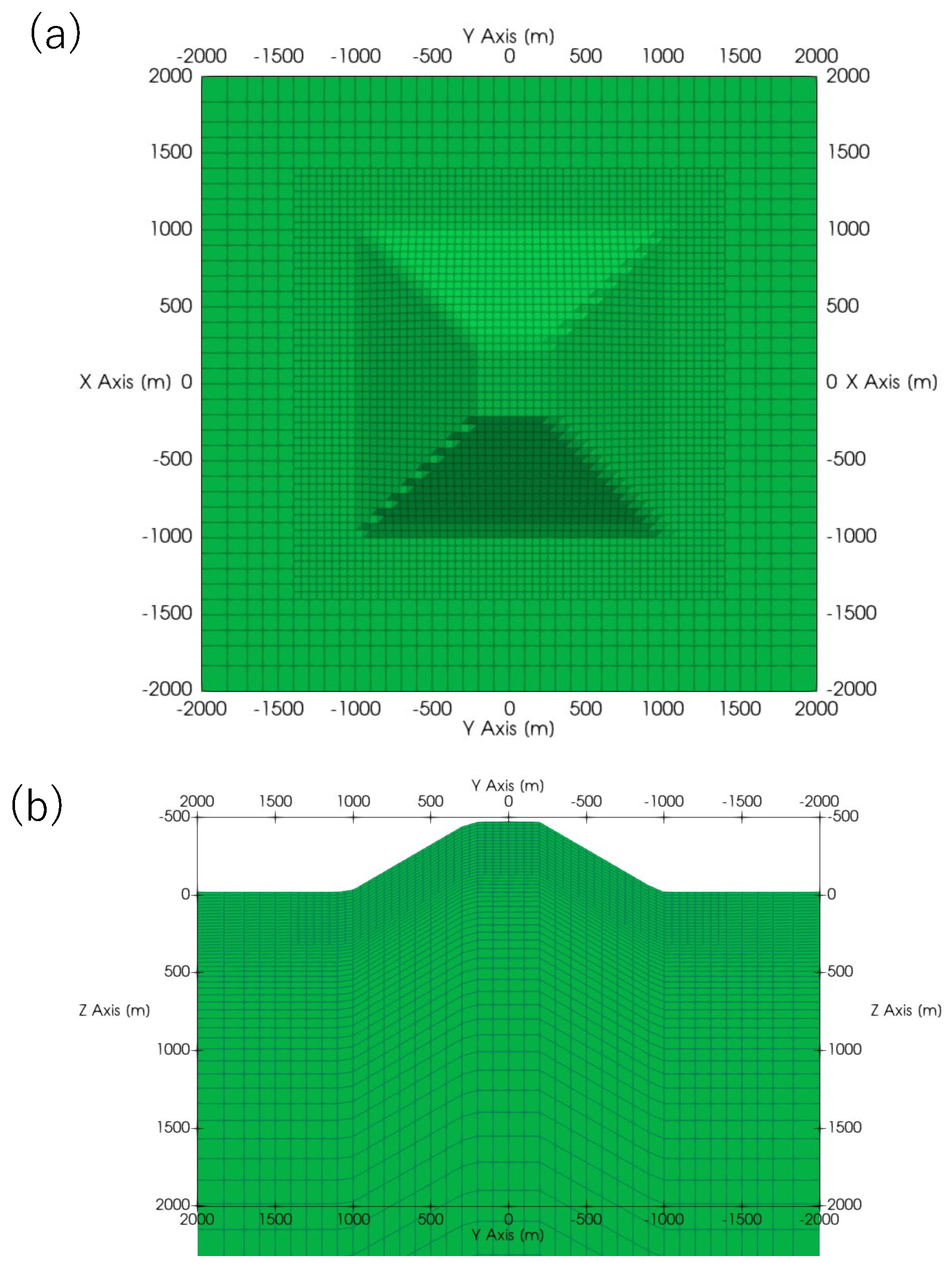
To evaluate if the developed program can consider topography, the trapezoidal hill model, which is often used to validate the effect of topography (e.g., Nam et al., 2007; Usui, 2015; Zhu et al., 2022, Figure 3) was adopted.

The minimum size of cells was 25 m ×25 m ×10 m and the total number of cells was 519,456. The resistivity in the air and the subsurface was ${10}^6$ and 100 $\mathsf{\Omega }\mathrm{m}$ respectively. The calculated frequency was 2 Hz. These conditions are the same as previous works (Nam et al., 2007; Usui, 2015; Zhu et al., 2022). The computer we used was Precision 3630 Tower (CPU: Intel® Core™ i7-9700 CPU 3.00GHz, RAM:16GB).

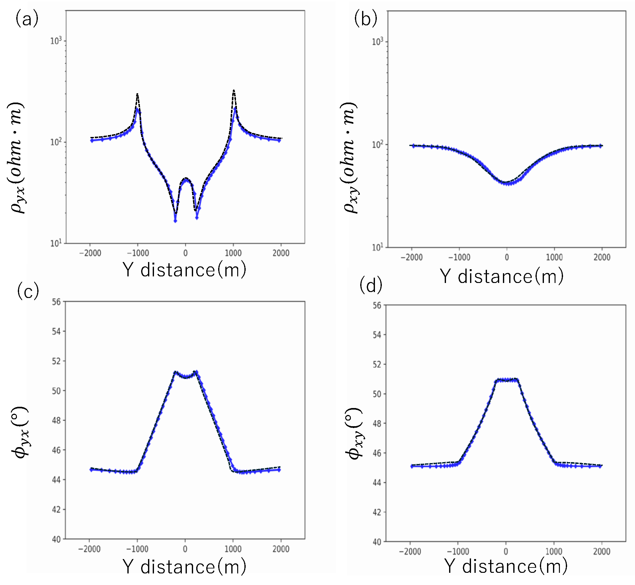
The results are shown in Figure 4. The results are compared to Zhu et al. (2022). Except for some points, these results are mostly consistent with each other. The gaps between them would be caused by the difference in the discretization method, as which Zhu et al. (2022) adopted FEM, and the size of cells. However, since the differences are quite small, it would not influence when the inversion is performed.

Figure 3. (a) XY and (b) YZ plane with used mesh of trapezoidal model in Nam et al. (2007).

Figure 3. (a) XY and (b) YZ plane with used mesh of trapezoidal model in Nam et al. (2007).

Figure 4. (a) Apparent resistivity of YX mode and (b) XY mode. (c) The phase of YX mode and (d) ZY mode of 2 Hz. Blue lines and diamonds denote our results. Black dashed lines represent the result in Zhu et al. (2022).

Figure 4. (a) Apparent resistivity of YX mode and (b) XY mode. (c) The phase of YX mode and (d) ZY mode of 2 Hz. Blue lines and diamonds denote our results. Black dashed lines represent the result in Zhu et al. (2022).

Forward Modelling Considering Resistivity Heterogeneity

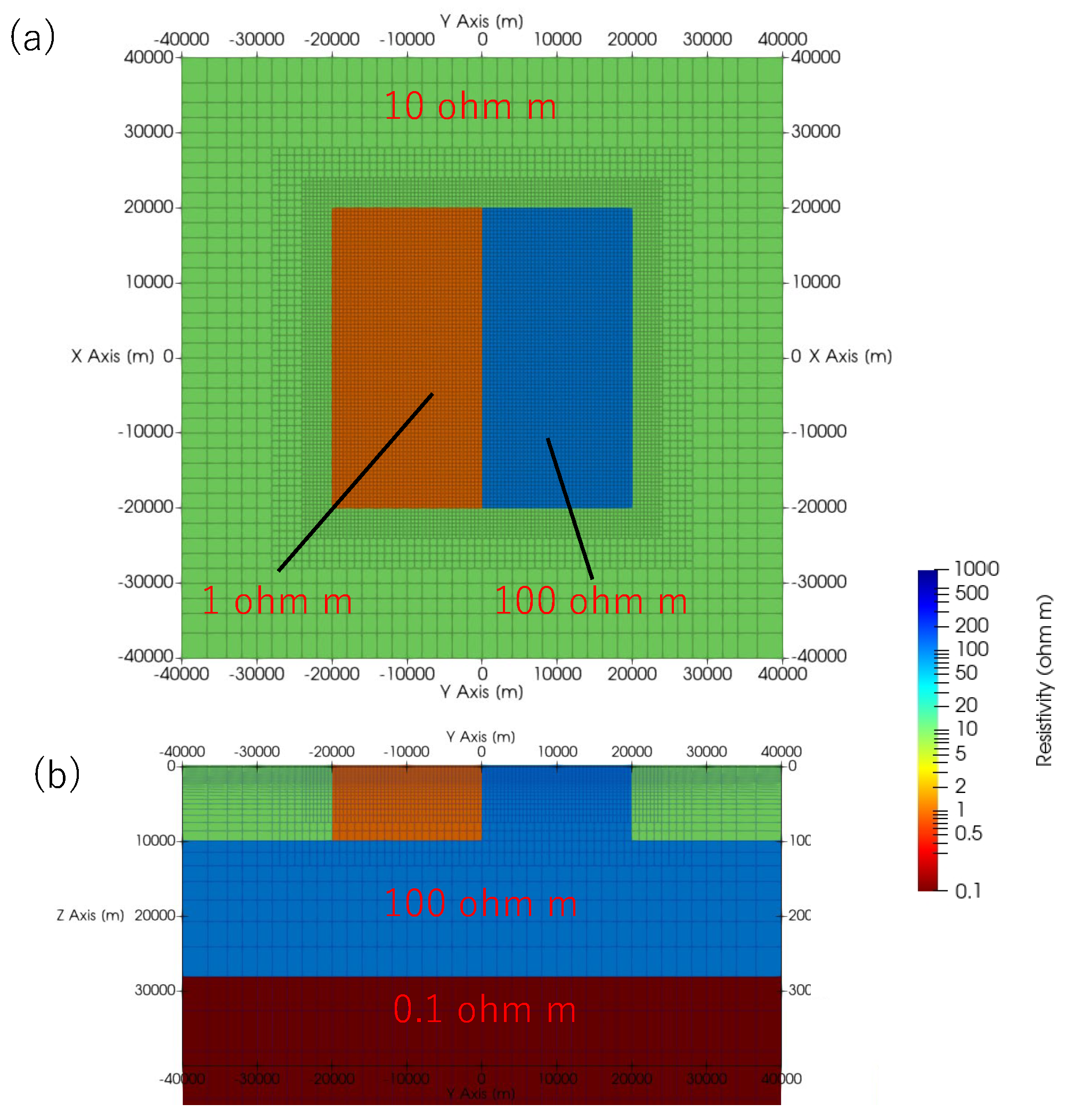
As a test case for heterogeneity of subsurface resistivity, the model in Mackie et al. (1993) was adopted (Figure 5). The total number of cells was 370,712, with minimum size of cells 500 m ×500 m ×200 m. The resistivity in the air and the subsurface was ${10}^6$ $\mathsf{\Omega }\mathrm{m}$. The compared frequency was 10 and 1000 s. The computer used is the same one used in the Trapezoidal hill model.

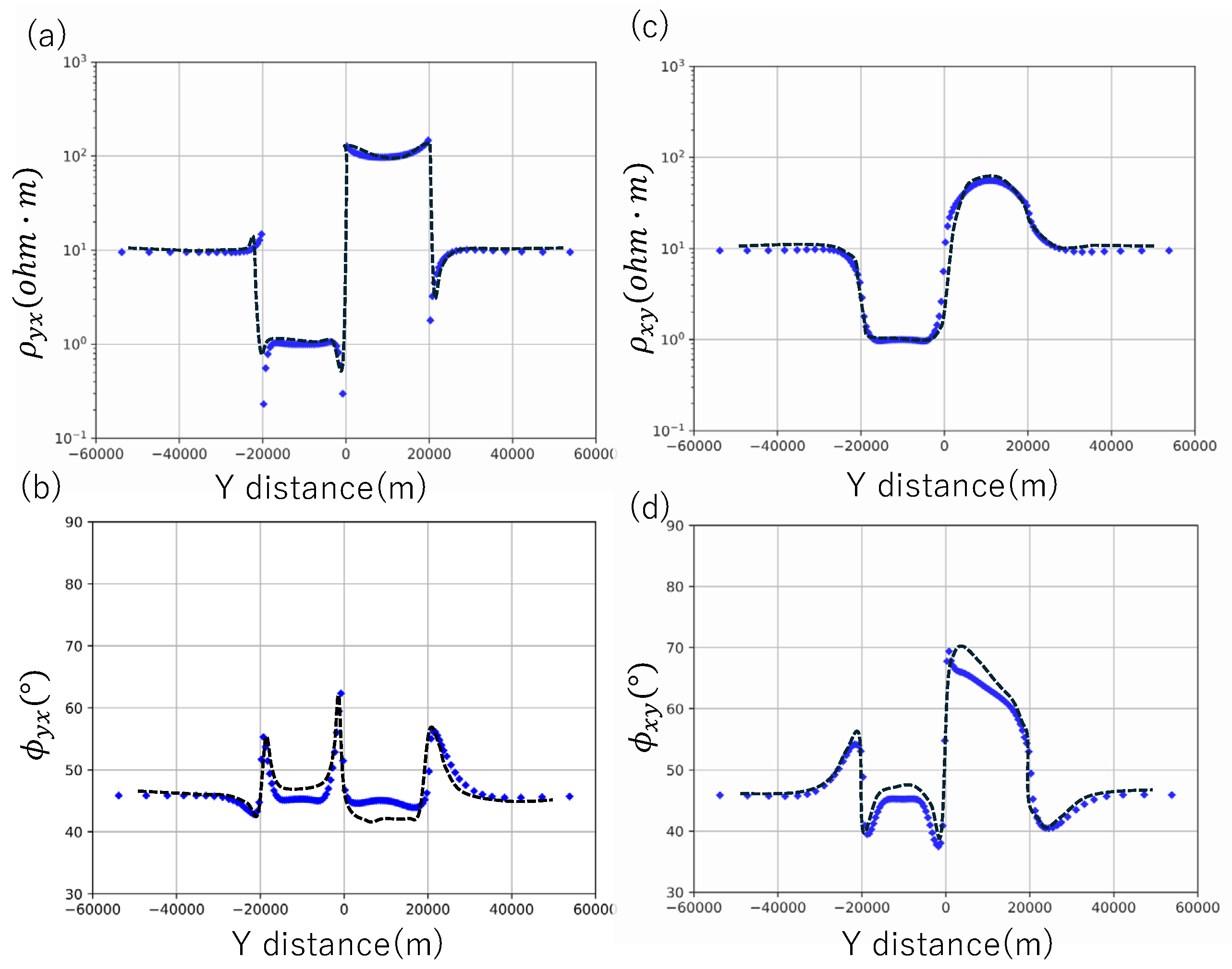
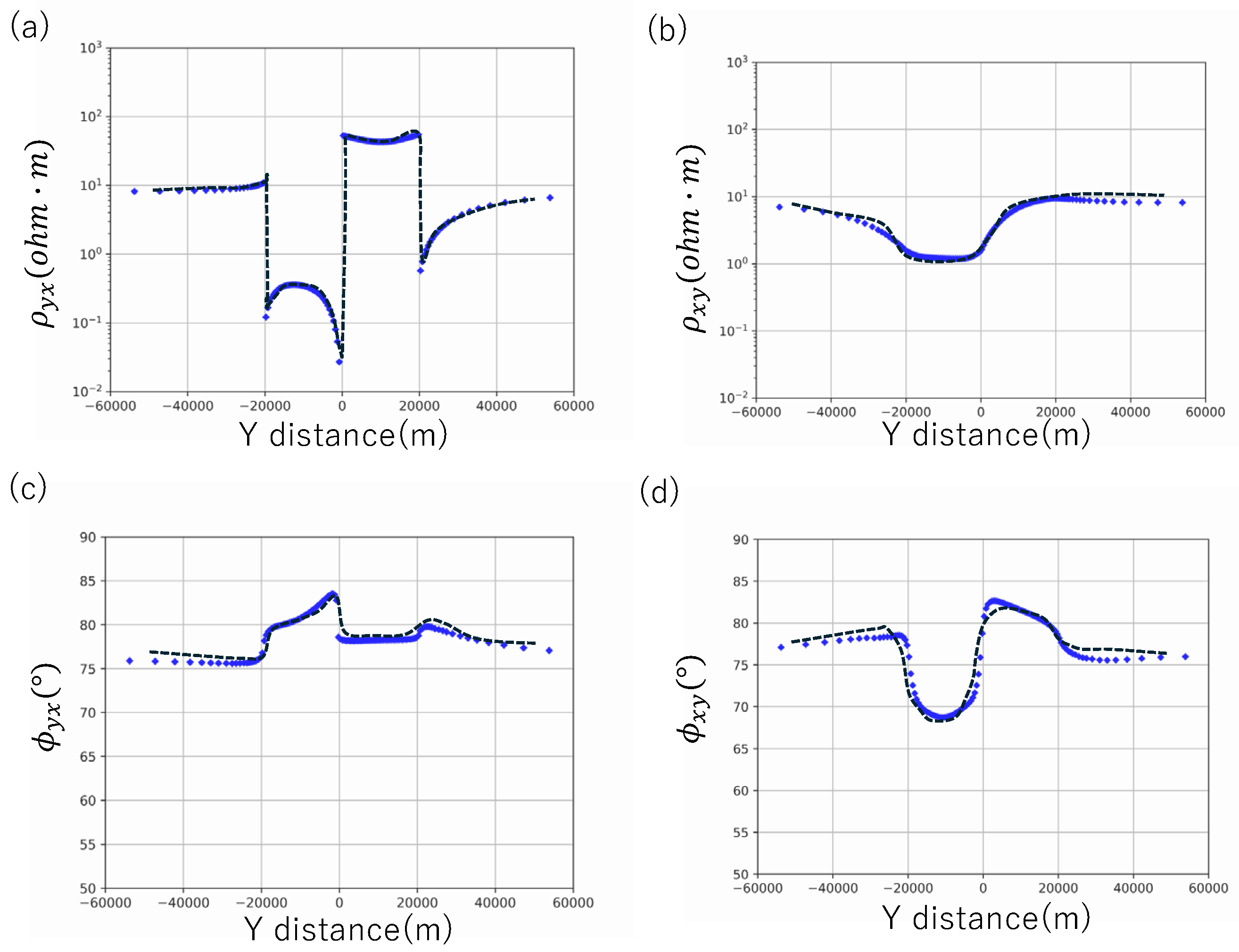
The results of Apparent resistivity and phase in cross sections along the Y direction at X=0 m for periods of 10 and 1000 s are compared with Mackie et al. (1993) in Figure 6 and Figure 7. While there are some small differences, the results are in good agreement with those of Mackie et al. (1993).

Figure 5. (a) XY and (b) YZ plane of the resistivity structure model in our forward calculation after Mackie et al. (1993). Transparent black lines denote cell edges.

Figure 5. (a) XY and (b) YZ plane of the resistivity structure model in our forward calculation after Mackie et al. (1993). Transparent black lines denote cell edges.

Figure 6. (a) Apparent resistivity of YX mode and (b) XY mode. (c) The phase of YX mode and (d) ZY mode of 10 s. Blue diamonds denote our results. Black dashed lines represent the result in Mackie et al. (1993).

Figure 6. (a) Apparent resistivity of YX mode and (b) XY mode. (c) The phase of YX mode and (d) ZY mode of 10 s. Blue diamonds denote our results. Black dashed lines represent the result in Mackie et al. (1993).

Figure 7. (a) Apparent resistivity of YX mode and (b) XY mode. (c) The phase of YX mode and (d) ZY mode of 1000 s. Blue diamonds denote our results. Black dashed lines represent the result in Mackie et al. (1993).

Figure 7. (a) Apparent resistivity of YX mode and (b) XY mode. (c) The phase of YX mode and (d) ZY mode of 1000 s. Blue diamonds denote our results. Black dashed lines represent the result in Mackie et al. (1993).

Inversion for Dublin Secret Model 2

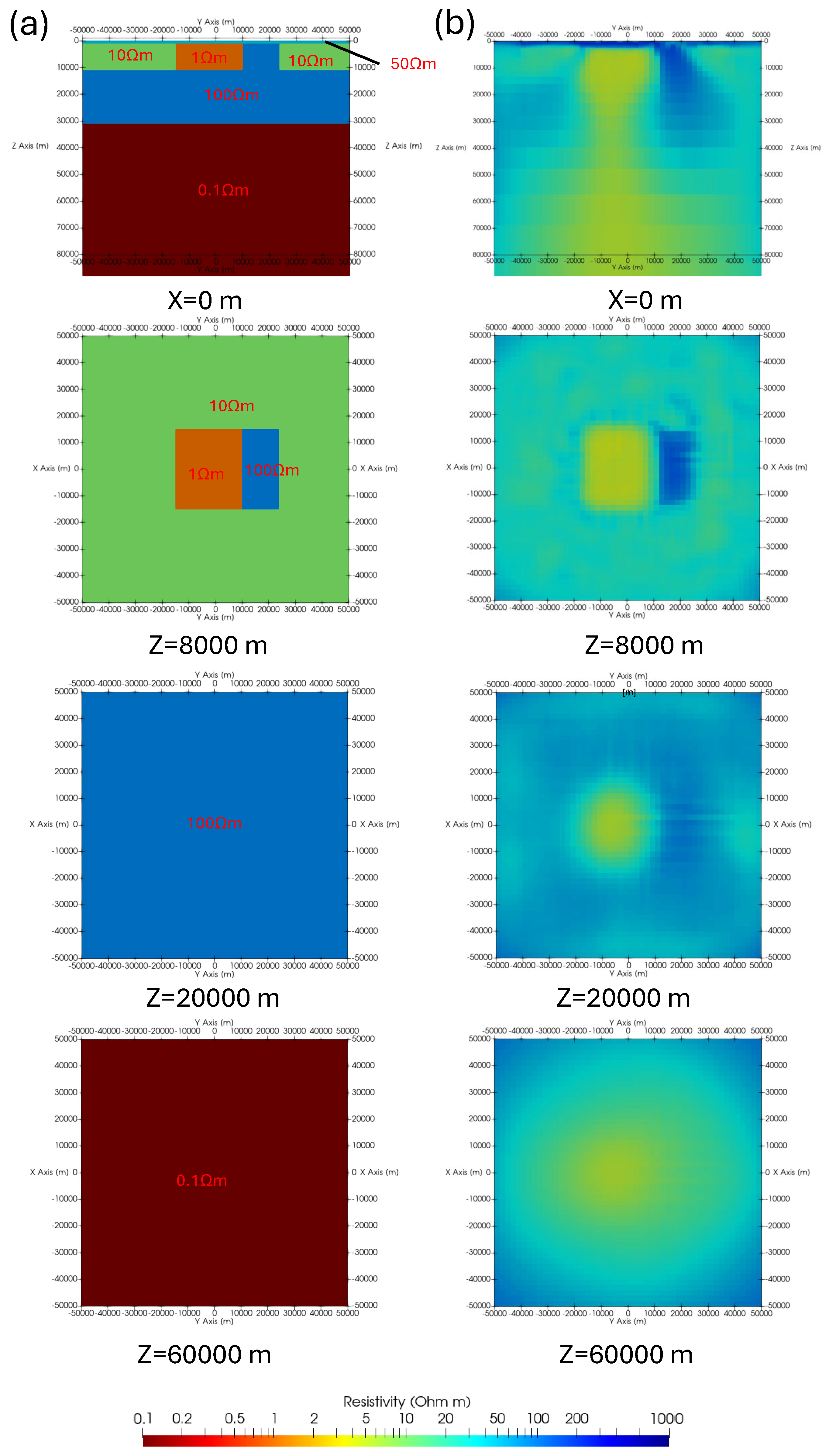
The author performed inversion using Dublin Secret Model 2 (DSM2) in Miensopust et al. (2013).This model was used as a comparison between different programs. The synthetic observed data of impedance tensor are openly available in Miensopust et al. (2013). The author used them as observed data.

The total number of cells was 223,784. The number of cells that were inverted as model parameters is 187,172. The number of degrees of freedom was 671,352. The minimum size of cells was 2000 m ×2000 m ×100 m. The initial resistivity was 100 $\mathsf{\Omega }\mathrm{m}$. The total number of calculated periods was 10, from 0.025 to 1000 s. The author initially set ${\alpha }^2$ to 100 and lowered it after the convergence criteria were achieved. The criteria were that the maximum change of model parameters or the change of objective function from the previous iteration was below 0.3 %. For simplicity, ${\beta }^2$ was set to the same value as ${\alpha }^2$. The computer for this calculation was Dell XPS 8950 (CPU: Intel® Core™ i7-12700K 3.60 GHz, RAM:64GB).

The results of the inverted resistivity structure compared to the true model are shown in Figure 8. The author adopted the model when ${\alpha }^2$ was 0.1, judging from the L-curved figure between RMS and model roughness (Figure 9) as in Usui et al. (2024). The resistive and conductive anomalies shallower than 10 km are inverted. While the conductive anomaly is connected to the one deeper than 30 km, this would be caused by low sensitivity under the conductive anomaly, as mentioned in (Usui 2015). In the conductive layer deeper than 30 km, The value of our result is a little high. This may be improved when data in longer periods are used.

Considering that the synthetic data is distorted according to Groom and Bailey (1989) and has 5% random noise of maximum impedance tensor value (Miensopust et al. 2013), the results of our program seem in agreement with the true model. A comparison of the results of Miensopust et al. (2013) would also support the agreement.

The total calculation time was about 20 hours. Usui (2015) calculated the same model in about 15 hours, with a number of degrees of freedom of 687,599, roughly the same as our calculation. Our calculation was performed without MPI parallelization, while one in Usui (2015) did with it. Nevertheless, we could obtain the results at a comparable time as Usui (2015), although the conditions of computation, such as the computers and the total number of calculated frequencies, were different. Further, our calculation was conducted on an ordinary personal computer. They would suggest the efficient performance of our program.

Figure 8. Each cross-section of the true DSM2 model in Miensopust et al. (2013) and our results. (a) True Model and (b) Our inversion results.

Figure 8. Each cross-section of the true DSM2 model in Miensopust et al. (2013) and our results. (a) True Model and (b) Our inversion results.

Figure 9. The L-curve picture of our inversion results. The vertical axis and horizontal axis are RMS and model roughness in each ${\alpha }^2$, respectively. We chose ${\alpha }^2=0.1$(red one) as our final result.

Figure 9. The L-curve picture of our inversion results. The vertical axis and horizontal axis are RMS and model roughness in each ${\alpha }^2$, respectively. We chose ${\alpha }^2=0.1$(red one) as our final result.

Conclusion

References

1. Dong, Hao, and Gary D. Egbert. 2019. “Divergence-Free Solutions to Electromagnetic Forward and Adjoint Problems: A Regularization Approach.” Geophysical Journal International 216 (2): 906–18. [CrossRef]
2. Fujiwara, Maki, Masahiro Yoshida, and Seiji Fujino. 2006. “BiCGSafe Method with Crout Version of ILU Decomposition Giving Triple Safe Keys for Convergence.” IPSJ Transactions on Advanced Computing Systems 47 (7): 52–60.
3. Groom, Ross W, and Richard C Bailey. 1989. “Decomposition of Magnetotelluric Impedance Tensors in the Presence of Local Three-Dimensional Galvanic Distortion.” JOURNAL OF GEOPHYSICAL RESEARCH 94 (B2): 1913–25.
4. Jacobi, Benoît, Gaël Guennebaud, and other contributor. 2024. “Eigen.”, https://eigen.tuxfamily.org/.
5. Jahandari, H., and C. G. Farquharson. 2015. “Finite-Volume Modelling of Geophysical Electromagnetic Data on Unstructured Grids Using Potentials.” Geophysical Journal International 202 (3): 1859–76. [CrossRef]
6. Kashiwagi, Masahide. 2024. “Kv - a C++ Library for Verified Numerical Computation.”, http://verifiedby.me/kv/.
7. Kelbert, Anna, Naser Meqbel, Gary D. Egbert, and Kush Tandon. 2014. “ModEM: A Modular System for Inversion of Electromagnetic Geophysical Data.” Computers and Geosciences 66 (May):40–53. [CrossRef]
8. Key, Kerry W., Steven C. Constable, and Chester J. Weiss. 2006. “Mapping 3D Salt Using the 2D Marine Magnetotelluric Method: Case Study from Gemini Prospect, Gulf of Mexico.” Geophysics 71 (1). [CrossRef]
9. Kingma, Diederik P., and Jimmy Ba. 2014. “Adam: A Method for Stochastic Optimization,” December. http://arxiv.org/abs/1412.6980.
10. Mackie, Randall L, Theodore R Madden, and Wannamaker Philip E. 1993. “Three-Dimensional Magnetotelluric Modeling Using Difference Equations - Theory and Comparisons to Integral Equation Solutions.” GEOPHYSICS. Vol. 58. http://segdl.org/.
11. Miensopust, Marion P., Pilar Queralt, Alan G. Jones, Dmitry Avdeev, Anna Avdeeva, Ralph Uwe Börner, David Bosch, et al. 2013. “Magnetotelluric 3-D Inversion-a Review of Two Successful Workshops on Forward and Inversion Code Testing and Comparison.” Geophysical Journal International 193 (3): 1216–38. [CrossRef]
12. Mitsuhata, Yuji, and Toshihiro Uchida. 2004. “3D Magnetotelluric Modeling Using the T-Ω Finite-Element Method.” Geophysics 69 (1): 108–19. [CrossRef]
13. Nam, Myung Jin, Hee Joon Kim, Yoonho Song, Tae Jong Lee, Jeong-Sul Son, and Jung Hee Suh. 2007. “3D Magnetotelluric Modelling Including Surface Topography.” Geophysical Prospect 55 (2): 277–87. [CrossRef]
14. Ogawa, Yasuo. 2002. “ON TWO-DIMENSIONAL MODELING OF MAGNETOTELLURIC FIELD DATA.” Surveys in Geophysics 23:251–73.
15. O’Hara, Keith. 2024. “OptimLib.”, https://www.kthohr.com/optimlib.html.
16. Plessix, Rene Edouard. 2006. “A Review of the Adjoint-State Method for Computing the Gradient of a Functional with Geophysical Applications.” Geophysical Journal International. [CrossRef]
17. Sasaki, Yutaka. 2004. “Three-Dimensional Inversion of Static-Shifted Magnetotelluric Data.” Earth Planets Space. Vol. 56.
18. Siripunvaraporn, Weerachai, Gary Egbert, and Yongwimon Lenbury. 2002. “Numerical Accuracy of Magnetotelluric Modeling: A Comparison of Finite Difference Approximations.” LETTER Earth Planets Space. Vol. 54.
19. Siripunvaraporn, Weerachai, Gary Egbert, Yongwimon Lenbury, and Makoto Uyeshima. 2005. “Three-Dimensional Magnetotelluric Inversion: Data-Space Method.” Physics of the Earth and Planetary Interiors 150 (1-3 SPEC. ISS.): 3–14. [CrossRef]
20. Takakura, Shinichi. 2014. “Estimation of a Regional Geothermal System by the Electromagnetic Exploration.” BUTSURI-TANSA 67 (3): 195–203.
21. Toh, Hiroaki, Adam SCHULTZ, and Makoto Uyeshima. 2000. “Electromagnetic Induction in Fully Heterogeneous Spheres Using the Staggered Grid Finite Difference Method.”.
22. Uchida, Toshihiro. 2022. “Consideration on Three-Dimensional Inversion of Magnetotelluric Data by Finite-Difference Modeling Including Topography: Data Interpretation at Northern Hakkoda Area.” Journal of the Geothermal Research Society of Japan 44 (1): 7–21.
23. Uchida Toshihiro, and Yusuke Yamaya. 2023. “Three-Dimensional Finite-Element and Finite Difference Inversions of Magnetotelluric Data: Application at Northern Hakkoda Geothermal Area.” Journal of the Geothermal Research Society of Japan 45 (3): 175–94. [CrossRef]
24. Usui, Yoshiya. 2015. “3-D Inversion of Magnetotelluric Data Using Unstructured Tetrahedral Elements: Applicability to Data Affected by Topography.” Geophysical Journal International 202 (2): 828–49. [CrossRef]
25. Usui, Yoshiya, Makoto Uyeshima, Hideaki Hase, Hiroshi Ichihara, Koki Aizawa, Takao Koyama, Shin’ya Sakanaka, et al. 2024. “Three-Dimensional Electrical Resistivity Structure Beneath a Strain Concentration Area in the Back-Arc Side of the Northeastern Japan Arc.” Journal of Geophysical Research: Solid Earth 129 (5). [CrossRef]
26. Zhu, Xiaoxiong, Jie Liu, Yian Cui, and Chunye Gong. 2022. “A Scalable Parallel Algorithm for 3-D Magnetotelluric Finite Element Modeling in Anisotropic Media.” IEEE Transactions on Geoscience and Remote Sensing 60. [CrossRef]