1. Introduction
Multi-objective optimization problems (MOPs), characterized by their inherent complexity and conflicting objectives, necessitate the development of efficient strategies to balance these diverse criteria. In response to this challenge, a multitude of algorithms have been devised, each aiming to effectively address MOPs. Notably, Differential Evolution (DE) [
1] has emerged as a promising contender within the realm of multi-objective optimization, exhibiting remarkable performance and demonstrating its potential to efficiently navigate the complex landscape of conflicting objectives. A detailed survey of some DE-based MOEAs has been conducted [
2], discussing their advantages and disadvantages. Most of these methods employ the widely used DE/rand/1/bin variant. While they have demonstrated effectiveness in accelerating the search and enhancing results, the review also reveals a latent issue with DE: the tendency to become trapped in local optimum fronts. To address this, diversity maintenance schemes must be incorporated into DE-based MOEAs. Additionally, handling the non-dominance relation between the trial individual and the target individual poses a challenge in these algorithms.
To tackle the aforementioned challenges, a novel algorithm, ILSDEMO, is proposed in this paper. It is built upon the "DE/best/1/bin" and "DE/best/1/exp" variants [
1] of DE. Prior experimental validation by E. Mezura-Montes [
3] revealed that, regardless of the problem characteristics, the "DE/best/1/bin" variant exhibited the highest competitiveness in terms of both quality and robustness of results among eight DE variants. Different from the "DE/best/1/bin" variant, the "DE/best/1/exp" variant allows larger mutation blocks to be inherited, which helps the algorithm escape from local optimal solutions on certain problems and enhances its global search capability. While several researchers have attempted to leverage these variants for solving MOPs [
4,
5], our approach distinguishes itself in several key aspects. Firstly, ILSDEMO initializes the parent population using the orthogonal design method [
6], which ensures a diverse initial population. Secondly, an archive population is employed to store non-dominated solutions, thereby maintaining a repository of promising candidates. Additionally, a k-nearest-neighbor rule is adopted to guarantee a uniformly distributed archive population in the objective space, enhancing the algorithm's ability to explore diverse regions of the search space. To generate a new parent population, an indicator-based selection mechanism is utilized, which leverages the performance indicators to identify promising individuals. Furthermore, the two DE variants and their corresponding parameters are selected in a self-adaptive manner, enabling the algorithm to adapt to the specific characteristics of the optimization problem. Lastly, a local search operator, specifically the q-Gaussian mutation[
7,
8], is applied to refine trial individuals that demonstrate superior performance compared to target individuals. This refinement step further enhances the algorithm's ability to find optimal solutions.
The remainder of the paper is organized as follows.
Section 2 defines several notable concepts pertaining to multi-objective optimization problems (MOPs) and briefly introduces the principles of indicator-based selection, differential evolution, and q-Gaussian mutation. In
Section 3, a comprehensive account of the ILSDEMO algorithm is provided, including a detailed description of its key components.
Section 4 presents an experimental investigation of the algorithm on the ZDT-series and DTLZ-series benchmarks, along with a comparative analysis of the results obtained with selected multi-objective evolutionary algorithms.
Section 5 summarizes the key findings and conclusions of the paper.
2. Preliminaries
Before delving into the details of the ILSDEMO algorithm, it is essential to introduce some fundamental concepts and theories that provide the necessary background for the algorithm's comprehension. These preliminary sections not only lay the foundation for understanding the principles and design of ILSDEMO but also aid in appreciating the algorithm's strengths and characteristics in solving multi-objective optimization problems. In the following sections, multi-objective optimization, orthogonal design, indicator-based selection, differential evolution, and Q-Gaussian mutation are introduced sequentially.
2.1. Multi-Objective Optimization
In contrast to single-objective optimization problems (SOPs), MOPs involves the optimization of multiple objectives. For the purpose of this discussion, it is assumed that all objectives are to be minimized. The problem can be formulated using Formula 1.
where
is a vector with n decision variables,
,
, …,
are objective functions,
,
, …,
are constraint functions. The decision space can be denoted as
. A solution in S is called a feasible solution. The objective space can be represented as
.
For the sake of facilitating the forthcoming discussion, we hereby present a comprehensive compilation of mathematical terminologies in MOO below.
Definition 1 (Pareto Dominance,
)
Definition 2 (Non-dominated, ~)
Definition 3 (Non-dominated set, NDS)
The non-dominated set, denoted as
Definition 4 (Pareto optimal solution)
A feasible solution is called a Pareto optimal solution,
Definition 5 (Pareto optimal set, PS)
The Pareto optimal set, denoted as, is the set of all Pareto optimal solutions.
Definition 6 (Pareto front, PF)
The Pareto front is defined as.
In accordance with definition 5, PS is the ultimate goal of optimization. However, the PS, especially for continuous MOPs, cannot be completely represented owing to the enormous amount of solutions. Moreover, too many solutions make no sense to help decision makers. Therefore, an appropriate selection for MOPs is to find a non-dominated set representing the Pareto optimal set as far as possible.
2.2. Orthogonal Design
The experimental design is an efficient approach for organizing experiments to enable the analysis of obtained data, leading to valid and objective conclusions [
9,
10]. In experimental designs, the decision variables are designated as factors, and the range of each factor is partitioned into multiple levels. Subsequently, all possible combinations of factors across all levels are tested, ultimately leading to the selection of the optimal combination. Given
n factors at
q levels, the total number of combinations is calculated as
. When
n and
q are
small, evaluating all combinations may be feasible. However, for a large number of factors and levels, testing all combinations becomes impractical. Therefore, a representative subset of combinations is selected for evaluation. Orthogonal design (OD) was developed for this purpose and has been successfully employed in evolutionary algorithms [
11,
12].
In OD, an orthogonal table provides some representative combinations of the factors at different levels. Let Lm(q, c) be an orthogonal table for c factors and q levels, where L denotes a Latin square and m is the number of the constructed combinations of the levels (). In the orthogonal table with m rows and c columns, each column denotes a factor and each row indicates a combination of the levels regarding the factors. The orthogonal table has some characteristics: 1) every level has the same occurrence number, i.e., m/q times, in any column; 2) every combination of two levels with respect to two factors has the same occurrence number, i.e., m/q2; 3) the selected combinations are uniformly distributed over the whole space of all the possible combinations; 4) if any two columns are swapped, the altered table is still an orthogonal table; 5) if some columns are removed from the orthogonal, the modified table is still an orthogonal table. A positive integer j should be found to minimize m with a constraint c ≥ n (n is the number of decision variables).
In this study, the algorithm described in [
13] is employed to produce an orthogonal table
Lm(
q,
c). Each element of the table,
a (
i,
j), indicates the level of the
jth factor in the
ith combination in
Lm(
q,
c). If
c>
n, the last
c-
n columns will be deleted to get an orthogonal table with
n factors. An element of the table is calculated as formula 2.
Here, lj and uj are the lower bound and the upper bound of the jth decision variable respectively, and the domain is quantized q-1 fractions.
2.3. Indicator-Based Selection
Indicator-based selection emerged from IBEA was first proposed by Zitzler [
13]. IBEA is based on quality indicators where a function
I assigns each Pareto set approximation a real value reflecting its quality, and thus the optimization goal becomes the identification of a Pareto set approximation that minimizes (or maximizes)
I. IBEA only compares pairs of individuals instead of entire approximation sets. The main advantage of the indicator concept is that no additional diversity preservation mechanisms are required.
A binary quality indicator is a function that maps multiple Pareto set approximations to a real number, and can be used to compare the quality of two Pareto set approximations. The indicator also can be used to compare two single solutions, and thus can serve for the selection process of evolutionary algorithms. As suggested in the literature [
18,
14], the majority of the multi-objective ranking techniques in the literature are easily adaptable into binary quality indicators. Here, the epsilon indicator
, which will be utilized in the algorithm, is solely introduced. The indicator quantifies the difference in quality between two solutions. It is defined as formula 3.
In order to assign fitness to the individuals, one of the following two schemes can be chosen: 1) One approach is to simply sum up the indicator values for each individual paired with the rest of the population as shown in formula 4. 2) Another approach is to amplify the influence of dominating individuals over dominated ones as shown in formula 5. Here, the parameter
k is a scaling factor depending on the indicator and the problem.
The fitness values of the individuals produce a total ordering relation of the whole population
P. As proved by zitzler [
18],
is dominance preserving. Thus, selection can be performed on the population P according to the orders of the fitness values.
Definition 7 (Dominance preserving) A binary quality indicator I is denoted as dominance preserving if:
1), and
2)
2.4. Differential Evolution
Differential evolution, proposed by Storn and Price [
1], is one of the most popular meta-heuristic optimizers, capable of handling non-differentiable, nonlinear, high-dimensional, multimodal continuous optimization problems. It has a concise idea but a strong global convergence. DE generates offspring by perturbing solutions with scaled differences of randomly selected vectors instead of the operations of crossover and mutation used in conventional evolutionary algorithms [
15].
The proposed algorithm will utilize two variants of DE, namely DE/best/1/bin and DE/best/1/exp, which use binomial crossover and exponential crossover respectively [
1]. The main difference between binomial crossover and exponential crossover is the fact that the components inherited from the mutant vector are arbitrarily selected and usually scattered in binomial crossover while one gene block of the mutant vector is inherited in exponential crossover. The following two key program segments illustrate the procedures of them. Here,
D is the dimension of the decision variable; randint(1,
D) denotes generating a random integer number between 1 and
D;
r1 and
r2 are two randomly generated integers with uniform distribution and their values are lower than or equal to the population size, and mutually different; best is a randomly generated integer with uniform distribution and less than the size of the non-dominated solution set;
F and
CR represent the scaling factor and the crossover probability respectively.
Program segment 1
|
jrand = randint (1, D) |
| for j=1 to D do |
| if rand(0,1)<CR || j == jrand then |
|
Vji = Xjbest + F*(Xjr1-Xjr2) |
| else |
|
Vji=Xji
|
| endif |
| endfor |
| Program segment 2 |
|
j=randint (1, D) |
|
k=0 |
| do |
|
Vji = Xjbest + F*(Xjr1-Xjr2) |
|
j = (j+1) % D
|
|
k++ |
| while (rand(0,1)<CR && k<D) |
2.5. Q-Gaussian Mutation
The q-Gaussian distribution [
16] allows to control the shape of the distribution by setting a real parameter
q and can reproduce either finite second moment distributions, like the Gaussian distribution, or infinite second moment distributions, like the heavy tail Lévy distribution.
One of the most interesting properties of the Gaussian distribution is that it maximizes, under certain constraints, the Boltzman-Gibbs entropy which is defined as formula 6.
Because the Gaussian distribution cannot represent well correlated systems with an infinite second moment, Tsallis[
17] proposed a generalized entropy form as formula 7.
The q-Gaussian distribution arises when maximizing the generalized entropy form given by formula 7. The parameter
q controls the shape of the q-Gaussian distribution. The q-Gaussian distribution reproduces the usual Gaussian distribution for
q=1. When
q=(3+
m)/(1+
m) and 0<
m<∞, it becomes a Student’s t-distribution with
m degrees of freedom. The q-Gaussian reproduces the Cauchy distribution for
q = 2. When
q<1, the q-Gaussian distribution has a compact form. When -∞<
q<3, the q-Gaussian distribution density is given as formula 8.
In formula 8,
is defined as formula 9. The q-mean
and q-variance
are defined as formula 10 and formula 11 respectively.
is the normalization factor and
controls the width of the q-Gaussian distribution and is given by
. A random variable
x following a q-Gaussian distribution with
and
is denoted by
. The generalized Box-Muller method can be used to generate q-Gaussian distribution for -∞<
q<3. As described in [
11], larger values of
q result in longer tails of the q-Gaussian distribution. The algorithm given by [
11] is employed to mutate a promising individual.
3. The Proposed Method
3.1. The Motivation
In evolutionary algorithms, many metrics such as convergence, accuracy, speed, and stability are employed to measure the performance of the algorithm. Besides, uniformity of the PF also acts as an important performance metric in MOEAs. However, a single method cannot perform well in terms of all the metrics [
18]. Take three popular algorithms for example. NSGAII performs well on two-objective problems in terms of convergence. Nevertheless, it usually cannot reach desirable results on three-objective problems [
19]. SPEA2 also works well on two or three-objective problems, but has a deteriorated convergence and time performance with increasing number of objectives. PESAII[
20] performs well in terms of convergence, but like NSGAII, it also relies on the quality of the initial population, and when dealing with large-scale or high-dimensional optimization problems, the computational cost and implementation difficulty of the algorithm may increase significantly.
In order to get an overall promotion in multiple metrics, some ways from different perspectives are worth trying. In Pareto rank based methods, the running time of non-dominated sorting and maintaining the diversity of the obtained non-dominated front all can be the starting points to improve the performance. Moreover, it is preferable to employ simple and efficient variation operators, such as DE and particle swarm optimization, to improve the time performance of the algorithm. In addition, using different selection operators to adjust the selection pressure and employing local search operators to improve the accuracy of the results are also popular in recent years [
21]. Recently, self-adaptive parameters and strategies have received more and more attention due to their significant impacts on the performance of the algorithms.
Based on the above considerations, we propose a novel MOEA which mainly incorporates orthogonal design, self-adaptive DE, local search, indicator-based selection, and updating method using k-nearest-neighbor rule.
3.2. Population Initialization
The state of the initial population usually has an effect on the results. Experimental design methods such as uniform design and orthogonal design are statistically sound [
12] and popular in many disciplines.
In our method, orthogonal design is utilized to generate an initial population where the individuals scattered uniformly over the feasible solution space, so that the algorithm can evenly scan the search space and locate the promising solutions quickly.
3.3. Variation Operators
3.3.1. Self-Adaptive Differential Evolution
In self-adaptive DE, not only the two control parameters but also the strategies are determined self-adaptively to avoid early stagnation. More specially, the control parameters and the strategy are encoded into the individuals. Initially, the scaling factor and crossover probability are randomly initialized within [0.2, 0.8] and [0.7, 1.0] respectively. One of the strategies, DE/best/1/bin or DE/best/1/exp, is randomly assigned to every individual. At the end of each iteration, the means and variances of two parameter values collected from the improved individuals are calculated to build two Gaussian models. The unimproved individuals will be assigned new parameter values by sampling the Gaussian models. Moreover, the strategies of these individuals will be reinitialized according to the probabilities of the two strategies based on the improved individuals.
3.3.2. Local Search
The purpose of local search methods is to enhance the exploitation capability of the algorithm. Previous researches have been focused on local search in MOO. In [
22], a local search procedure was applied to new solutions but only a small number of neighborhood solutions were examined to prevent the local search procedure from spending almost all available computation time. In [
23], a gradient-based mathematical programming method was employed to perform the local search on the offspring population. In [
24], based on non-dominated sorting and crowding distance, local RBF (Radial Basis Function) surrogates were constructed around the sparse points, with the aim of accurately predicting the values of the objective function. In [
25], a PF model-based local search method was proposed to accelerate the exploration and exploitation of the PF. Different from other local search methods in the literature of MOEA, q-Gaussian mutation is used to perform exploitation once the trial individual is better than the target individual. But the replacement scheme is noticeable in view of the fact that the comparison of the solutions for MOPs is distinct from that of SOPs. In this algorithm, if the individual obtained by local search dominates the target individual, the latter will be replaced by the former. Otherwise, the target individual remains unchanged. In either case, the trial individual should be used to update the archive population in order to avoid neglecting possible improvement on the distribution of the archive population.
3.4. The Selection Operator
In SOPs, the selection operator is usually employed to adjust the proportion of the best individuals involved in the variation of the next generation. In MOPs, it has a similar effect. However, besides the convergence, the diversity of the parent population in the objective space should also be concerned. In NSGAII, the uniformity of the parent population is only maintained by the crowding selection performed on the part of the population in the early stage. Thus, the crowding distance cannot effectively reflect the density of a solution especially in three or more objective problems. In fact, using the same selection operator on the archive population, NSGAII only achieves acceptable performance in terms of diversity in two-objective problems. Fortunately, the deficiency is compensated via propagating the extreme solutions to the next generation. In contrast, indicator-based selection can achieve better uniformity in the whole parent population. Nevertheless, indicator-based selection is prone to suffer a loss of the extreme solutions. Thus, the performance deteriorates with a worse coverage. Moreover, the algorithm cannot perform further exploitation to the extreme solutions.
In this study, indicator-based selection is employed to generate a new parent population based on a union of the old parent population and the archive population. First, the duplicated individuals are eliminated from the union. Then, the extreme solutions will be ensured to survive to the new parent population via assigning small enough indicator values to them. In addition, the formula 5 is converted into the formula 12 so as to keep the selection of indicator values in harmony with the objectives, i.e., minimization. Thus, if the number of the remaining individuals is not beyond the parent population size, all the individuals will be propagated into the next parent population. Moreover, the parent population may need to be supplemented by some new initialized individuals. Otherwise, the indicator-based selection will work. Specifically, an individual with a maximum indicator value is deleted from the union, and the indicator values of the other individuals are updated concurrently. The procedure is repeated until the number of the remaining individuals is equal to the parent population size.
3.5. The Updating Rule
Although indicator-based selection is an effective method in favor of finding a well-distributed solution set, it still cannot obtain ideal uniformity as well as some other algorithms such as SPEA2. Therefore, an updating criterion using the nearest neighbor will be introduced for the update of the archive population in both algorithms. In detail, when the number of non-dominated solutions exceeds the archive population size, the cumulative Euclidean distance (called density) to its k nearest neighbors for every non-dominated solution will be calculated. Here k is set to 2 * (m - 1), and m is the objective number. The individual with the smallest density will be removed. Meanwhile, the densities of other individuals are updated. Then, the procedure is repeated until the quantity of the rest is equal to the archive population size.
3.6. The Framework of the Proposed Algorithm
Based on the above design, the procedure of the proposed ILSDEMO algorithm for solving MOPs is summarized in Algorithm 1.
| Algorithm 1 ILSDEMO |
1: Set n=0. Initialize the population Pn{(Xi,Fi,CRi,Si),i∈[1,NP]} using OD
2: Evaluate Pn
3: Copy the non-dominated solutions to the archive population PA.
4: while the termination criteria are not satisfied do
5: Set n = n + 1
6: for i=1 to NP do
7: select r1≠r2 ∈{1, 2, …, NP} randomly
8: best∈{1,2,…,fsize} //fsize is the size of the non-dominated set in PA.
9: Perform program segment 1 or 2 using Si,Fi,CRi
10: Evaluate Vi
11: if f(Vi) is non-dominated by f(Xi) then
12: if f(Vi) dominates f(Xi) then
13: Mark f(Xi) as an improved individual
14: end if
15: Perform q-Gaussian mutation on Vi
16: Add Vi to PA using k-nearest neighbor rule
17: end if
18: if f(Vi) dominates f(Xi) then
19: Xi = Vi
20: end if
21: endfor
22: Build two Gaussian Models using the F and CR values collected from
the individuals improved by DE
23: Calculate the probabilities of the strategies based on the
individuals improved by DE
24: Generate Pn+1 based on Pn and PA using indicator-based selection.
25: Reinitialize F, CR, and S for the unimproved individuals according to
the above models
26: endwhile |
4. Experiments
In this section, the performance of ILSDEMO is experimentally investigated, compared with NSGAII, IBEA, and DEMO, which are renowned for their distinctive attributes, manifesting diverse strengths and applicability across various problem domains, commonly serving as benchmark algorithms for comparative analysis. The comparative assessment is conducted utilizing two comprehensive test suites and three rigorous performance metrics, with statistical analysis employed to discern the outcomes. All the experiments are implemented in VC6.0, Matlab 7.1, Sigmaplot 12.0 and run on Intel i5 760 2.8GHz machines with 4GB DDR3 RAM.
4.1. Performance Metrics
In general, the quality of the non-dominated sets should be evaluated according to the convergence and the diversity in the objective space. The convergence depicts the closeness of the final non-dominated solutions to the true PF, whereas the diversity aims at the uniformity and the coverage of the final solution set along the true PF. A number of performance metrics, such as hypervolume (HV) [
26], generational distance (GD) [
27], inverted generational distance (IGD) [
31], spacing metric (Spacing) [
28,
29], set coverage (SC), among others, have been proposed. However, none of the performance metrics can reliably evaluate both performance goals [
30]. Given that IGD and HV concurrently account for the convergence and diversity of the solution set[
31], while the Spacing metric precisely captures the uniformity of the distribution of the solution set in the objective space, these three metrics are selected for comparing the non-dominated solutions obtained by the four algorithms. A brief description of the metrics is given as follows.
1) HV metric
HV metric, originally proposed by Zitzler and Thiele [
32], computes the volume in the objective space covered by the non-dominated solutions and a reference point. Coello Coello, Van Veldhuizen and Lamont [
33] described it as the Lebesgue measure
of the union of hypercubes enwrapped by a non-dominated set
B and a bounding reference point
zr which is dominated by all points. The formalization is shown as formula 13. As elaborated by Knowles [
34], the hypervolume metric is the only unary indicator that is capable of detecting that solution set
A with a low indicator value is not better than
B with a high value.
In subsequent experiments, a fast algorithm termed HSO (Hypervolume by Slicing Objectives)[
34] will be utilized for the computation of hypervolume, and the difference in hypervolume with respect to a reference set
RS will be adopted as a performance indicator designated as
HV*. The indicator value is defined as formula 14. Hence, a smaller value of
HV* corresponds to a higher quality.
2) IGD
Suppose
P* and
P represent a uniformly sampled solution set along the true PF and a non-dominated solution set obtained by an algorithm respectively. The mean distance from
P* to
P is calculated as formula 15:
where
indicates the minimum Euclidean distance between
v and the points in
P. If
P* can represent the PF very well, the metric can measure both the convergence and the diversity while GD metric can only measure the convergence. A small value for IGD is desirable as it indicates better performance of the algorithm in terms of convergence and distribution.
3) Spacing
The Spacing metric measures how evenly the points in the approximation set are distributed in the objective space. An enhanced version of the metric will be employed, taking into account the Euclidean distances between the two extreme endpoints of the non-dominated front and their corresponding endpoints on the PF. A smaller spacing value indicates the solution set has a better spread. The metric is given by formula 16 where
and
are the Euclidian distances between the extreme solutions in PF and NDS,
denotes the distance between the adjacent solutions via sorting one objective, and
denotes the average of
,
Although the metric is utilized to measure the diversity of non-dominated set extensively, it only works well for two objective problems due to the calculation method of
di.
4.2. Parameters Settings
According to the preliminary experiments, the common parameters are set as follows: NP=50, NA=100 (150 for DTLZ-series), F∈[0.2, 0.8], CR∈[0.7,1.0], RUNs=30, Max_Evals=50000 (100000 for DTLZ-series). Here, NP represents the parent population size, NA denotes archive population size, F and CR are the scaling factor and crossover rate of DE respectively, RUNs and Max_Evals indicate the number of runs and evaluations in one run respectively. In addition, a factor k is set to 0.02 in indicator-based selection. In IBEA and NSGAII, NO (=50) indicates the offspring population size, PC (=0.8) and PM (=0.1) represent the probabilities of simulated binary crossover (SBX) and polynomial mutation respectively, eta_cross (=20) and eta_mut (=20) are the distribution indices of SBX and polynomial mutation respectively. In the computation of performance metrics, the objective values are normalized using the arctan function and subsequently mapped onto the interval [0, 1]. Additionally, the objective value of each reference point is set to 1.0.
4.3. Experimental Results and Discussions
In this section, the experimental results obtained by ILSDEMO, NSGAII, IBEA, and DEMO on the DTLZ-series and ZDT-series test instances are presented and discussed. The ZDT-series comprises two-objective problems, with the dimension of decision variables set to 30 for ZDT1, ZDT2, and ZDT3, and 10 for ZDT4 and ZDT6 in the conducted experiments. The DTLZ-series, on the other hand, represents scalable problems. For the DTLZ-series, the objective dimension is fixed at 3, with the dimension of decision variables set to 7 for DTLZ1, 12 for DTLZ2-6, and 22 for DTLZ7 respectively.
According to the HV* metric,
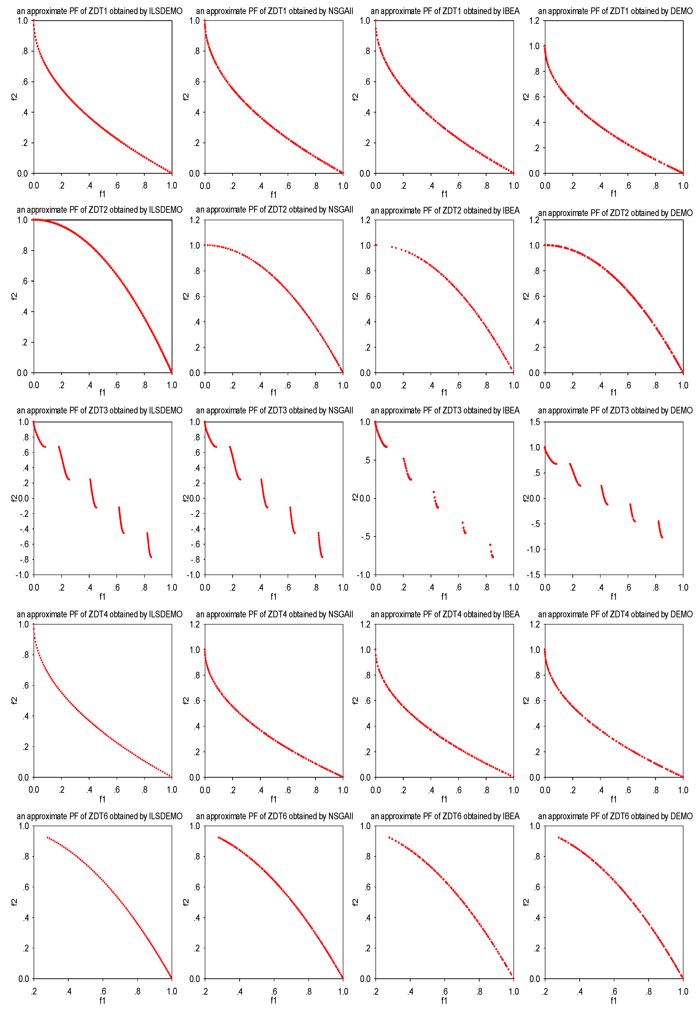
Figure 1,
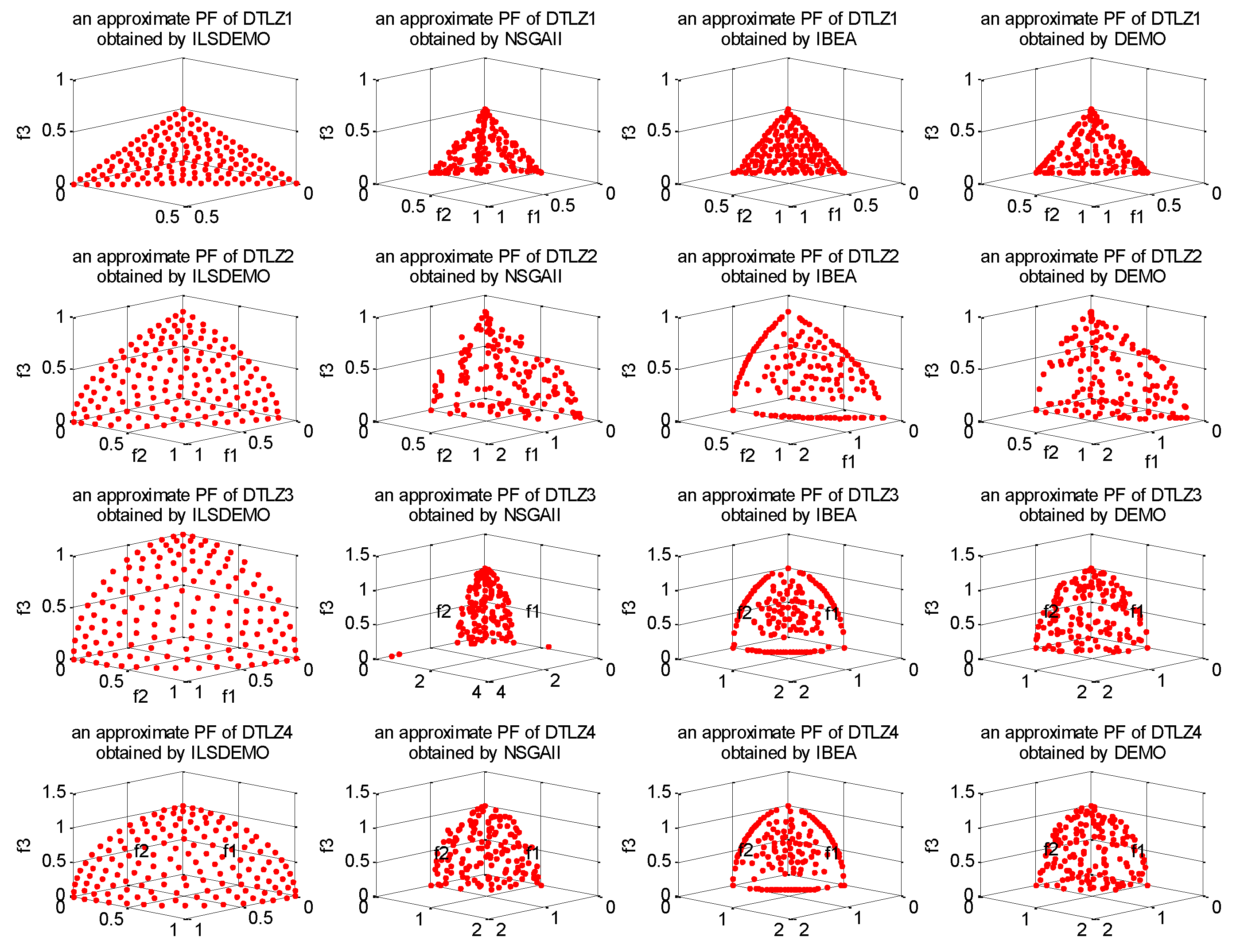
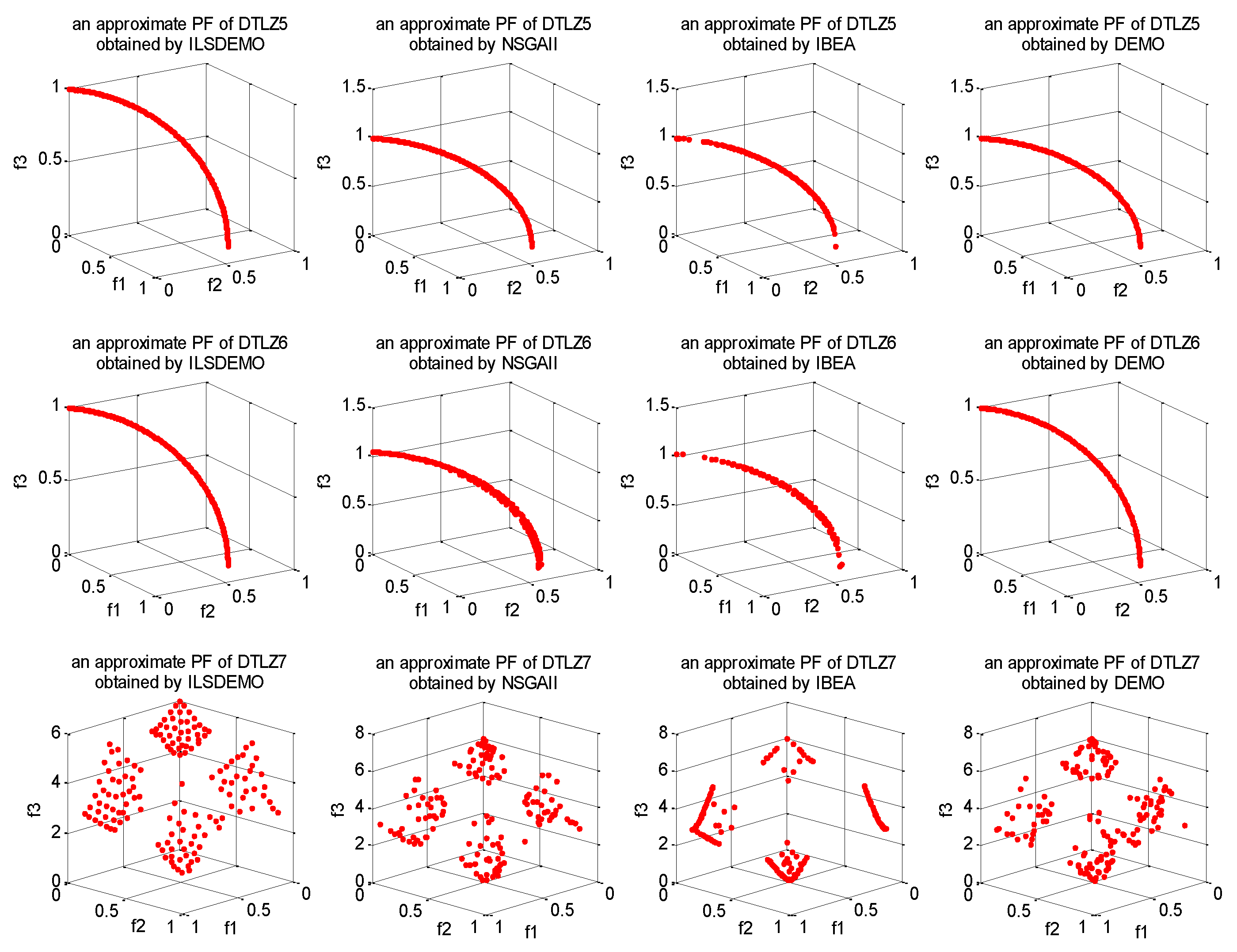
Figure 2, and
Figure 3 demonstrate the optimal approximations to the true PFs achieved by the four algorithms on the ZDT-series and DTLZ-series test instances.
Figure 1 reveals that the non-dominated solutions attained by ILSDEMO for the ZDT-series exhibit a more uniform distribution along the non-dominated front, indicating promising approximations across all algorithms. In contrast, NSGAII and DEMO exhibit seemingly inferior diversity, while IBEA maintains the worst distribution due to its inability to effectively retain extreme solutions, resulting in incomplete coverage of the non-dominated front.
As evident from
Figure 2 and
Figure 3, ILSDEMO achieves more accurate and uniform approximations to the true PFs of the DTLZ-series. Specifically, for DTLZ1, IBEA's solutions exhibit a more even distribution, while NSGAII maintains the worst distribution. For DTLZ2 and DTLZ4, NSGAII and DEMO display similar distributions, with IBEA exhibiting the worst distributions. While IBEA's solutions demonstrate a certain degree of uniformity in the centers of the fronts, significant gaps are observed between the centers and edges, along with the loss of some extreme points of the three objectives. For DTLZ3, NSGAII's approximate front is the worst due to outliers, while DEMO outperforms IBEA. For DTLZ5 and DTLZ6, ILSDEMO and DEMO yield similar distributions and accuracies, while IBEA produces the worst results. Finally, for DTLZ7, ILSDEMO approaches the true PF more evenly, while the non-dominated front obtained by NSGAII resembles that of DEMO.
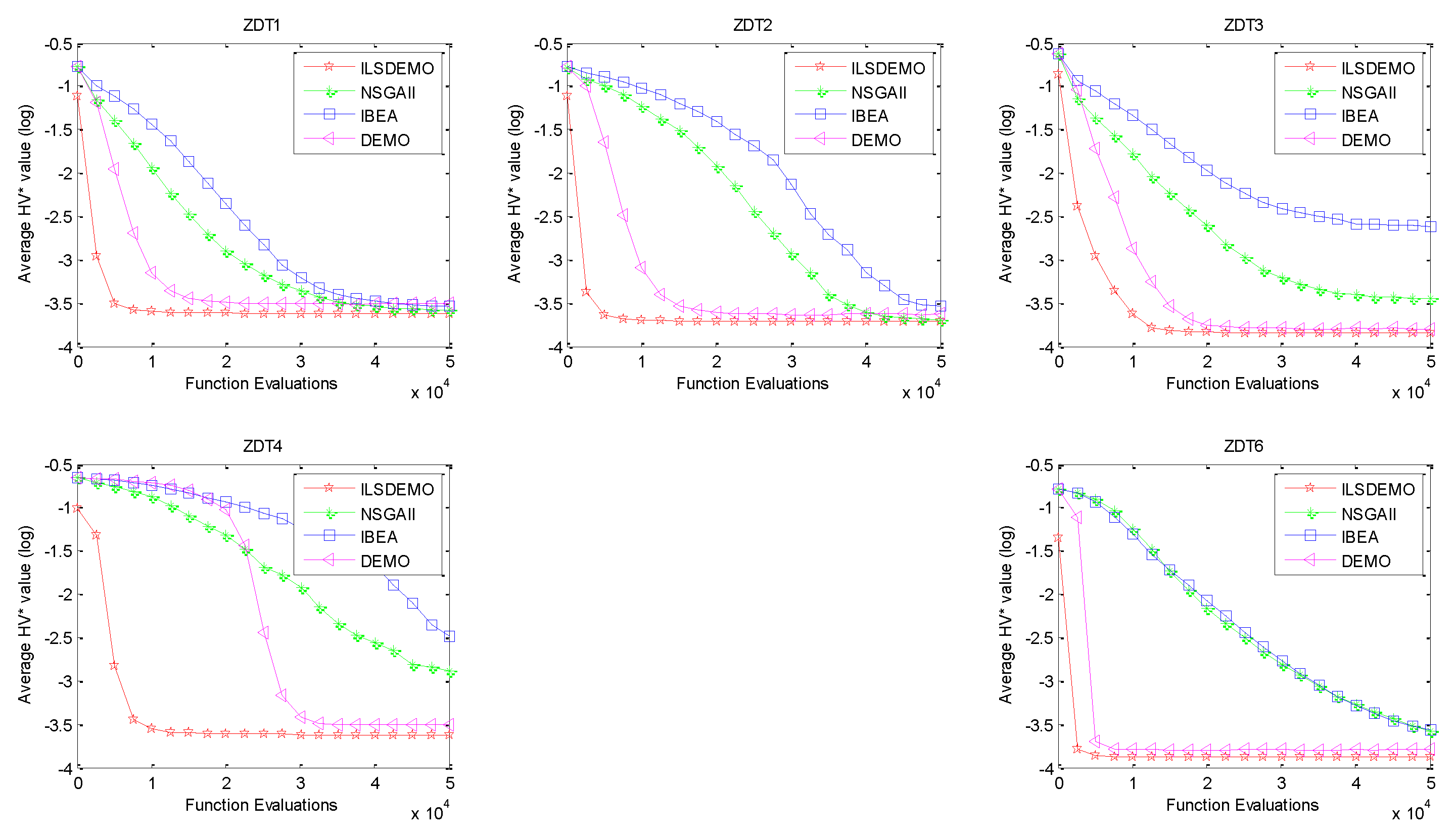
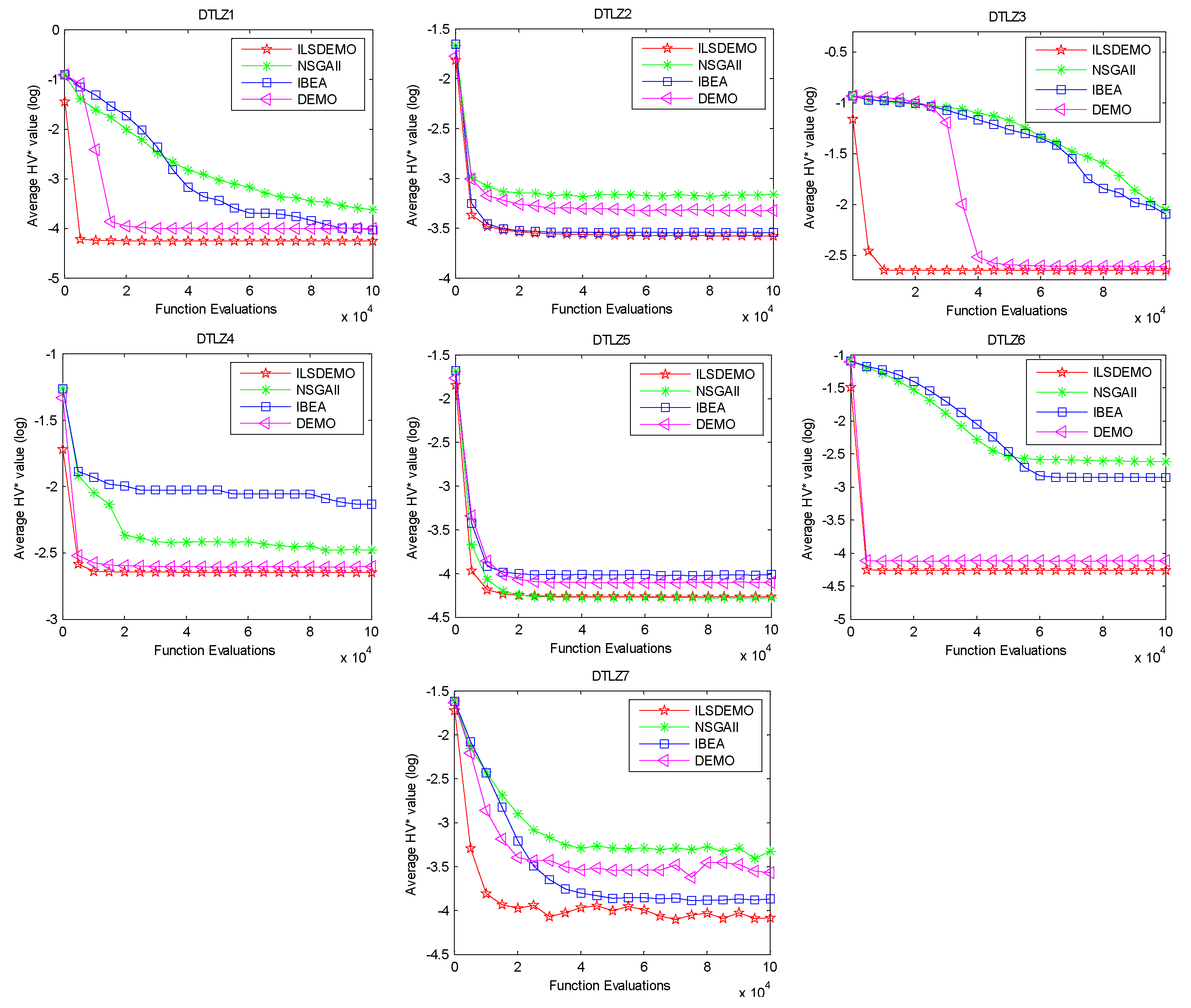
To gain further insight into the performance of ILSDEMO, a comparison with the other three algorithms is conducted based on the convergence speed, which is quantified by the average HV* values as a function of the number of function evaluations.
Figure 4 clearly demonstrates a consistent ranking in terms of convergence speed among the four algorithms: ILSDEMO exhibits the fastest convergence, followed by DEMO, NSGAII, and finally IBEA, which converges the slowest.
Figure 5 also confirms that ILSDEMO maintains its position as the fastest algorithm. Specifically, for DTLZ1, DTLZ3, and DTLZ7, ILSDEMO converges significantly faster than the other algorithms. However, for DTLZ2, IBEA converges only slightly slower than ILSDEMO. Similarly, for DTLZ4 and DTLZ6, DEMO converges with a minor lag behind ILSDEMO. Lastly, for DTLZ5, NSGAII performs almost on par with ILSDEMO.
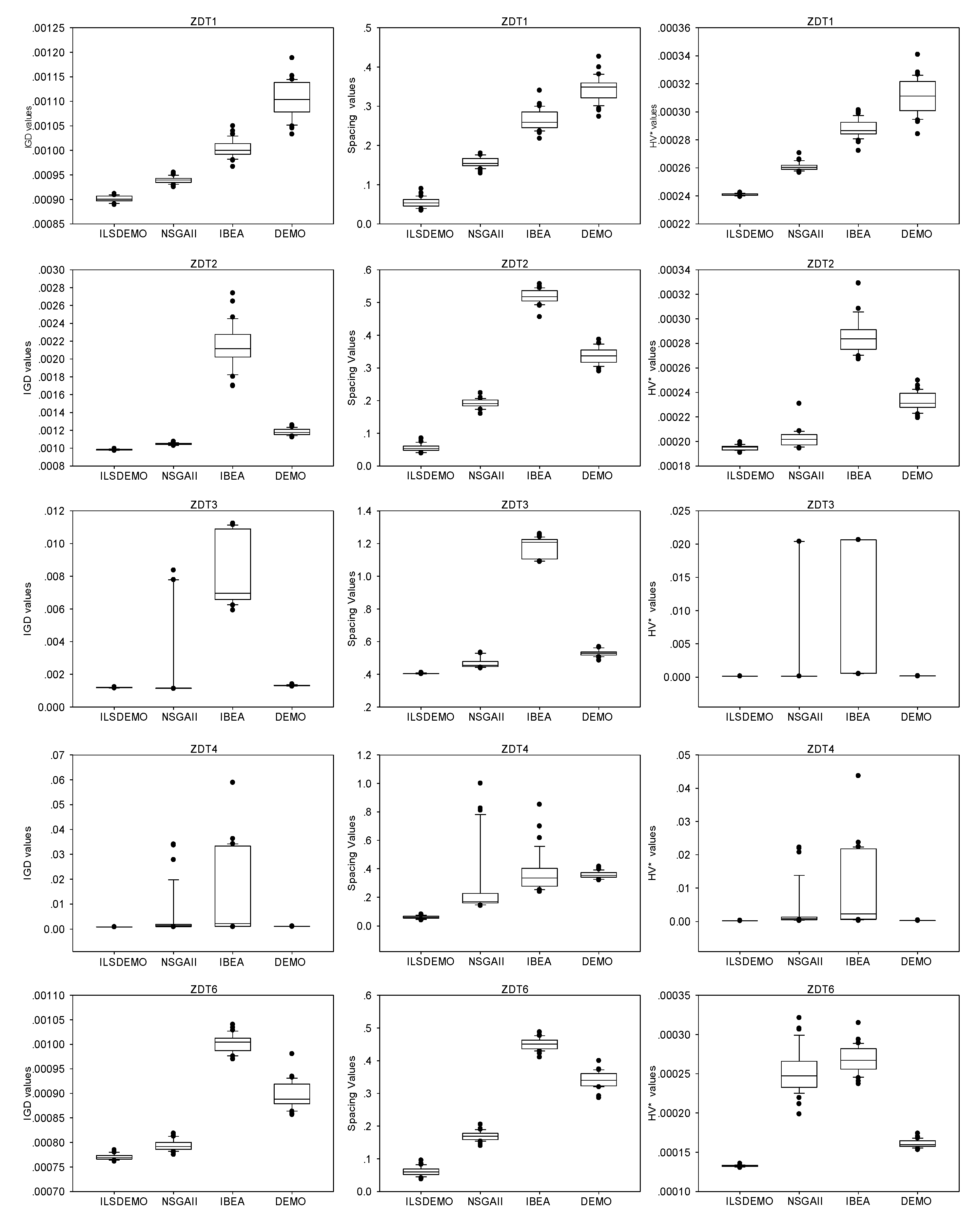
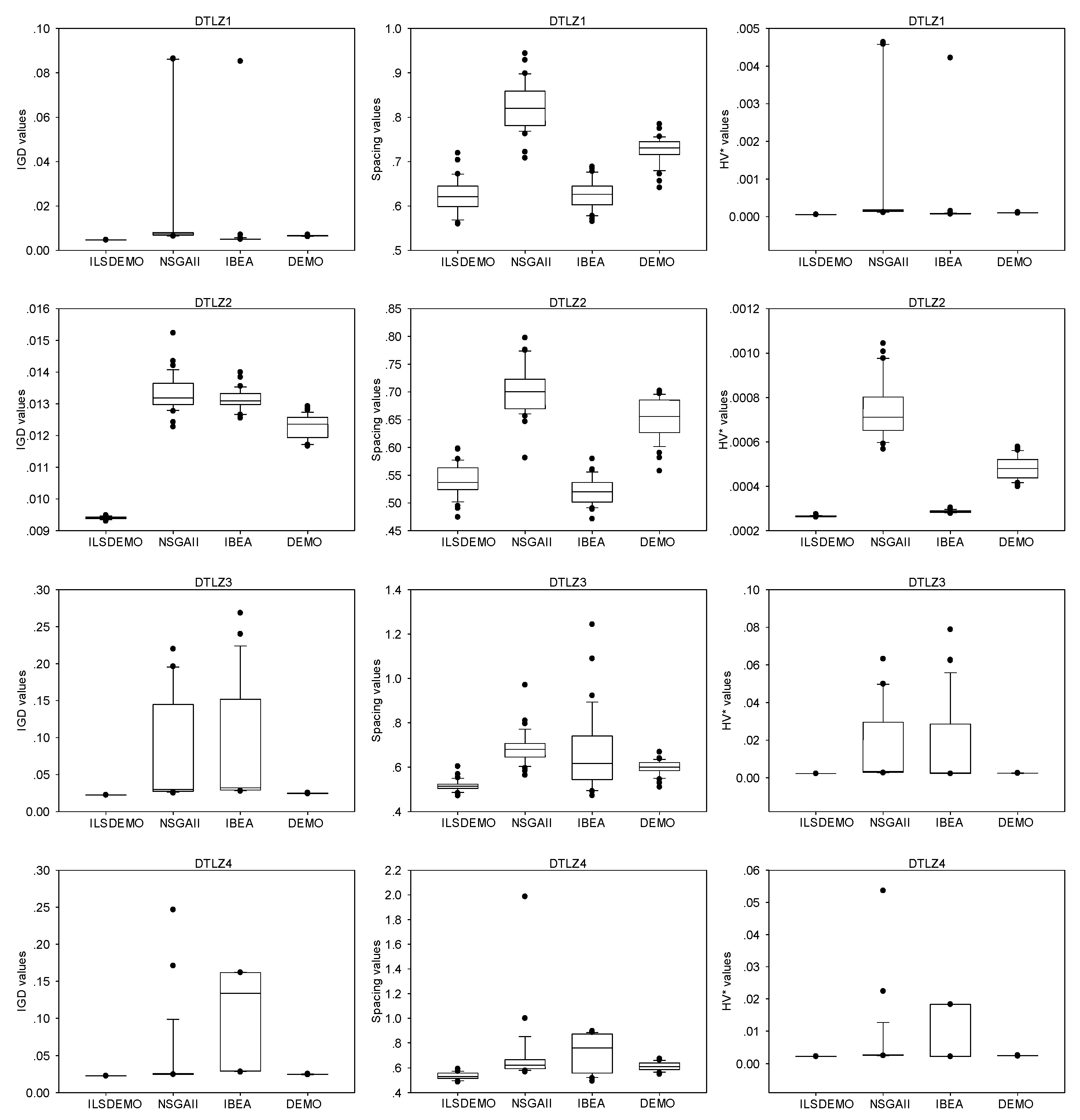
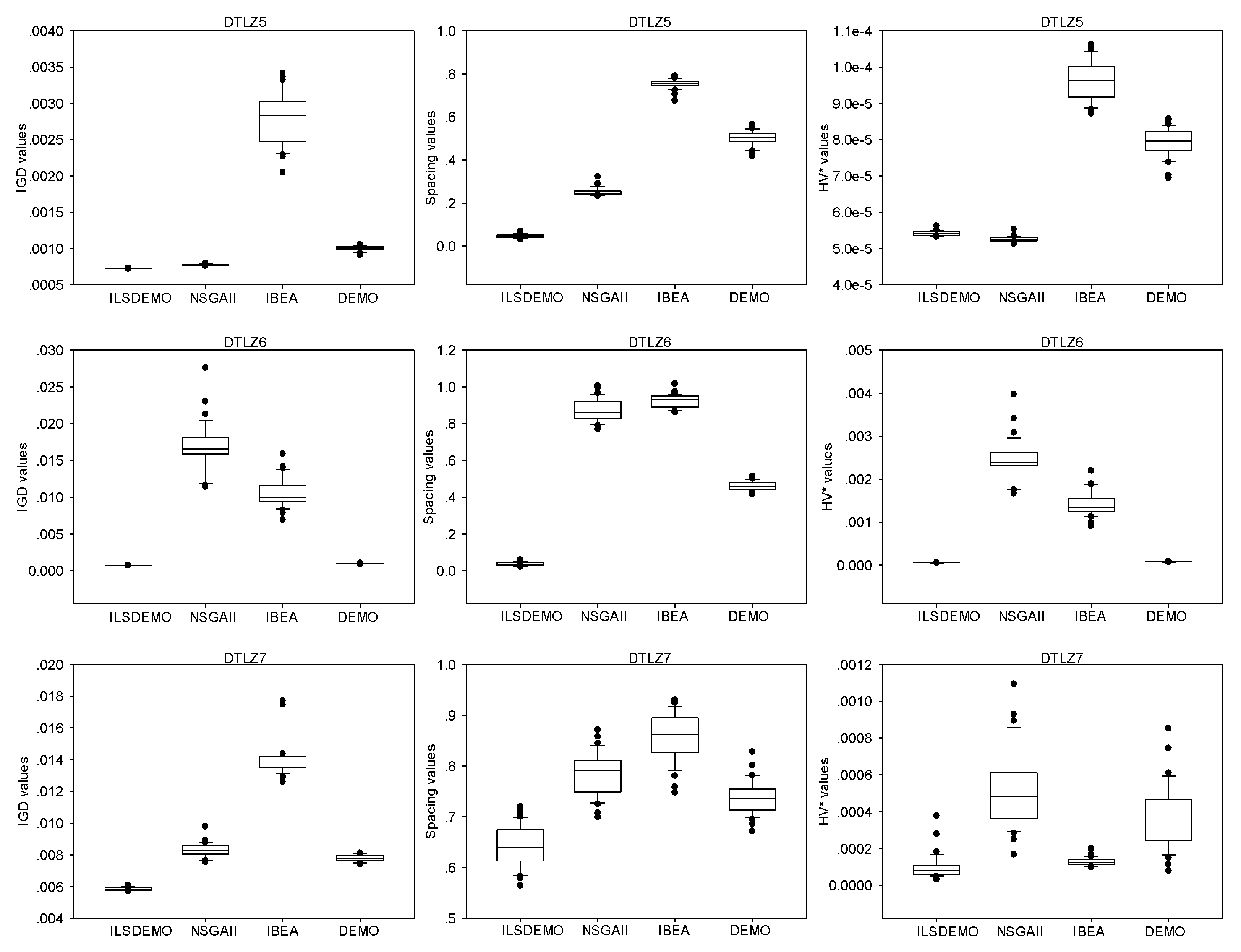
The box-plots presented in
Figure 6,
Figure 7, and
Figure 8 offer statistical evidence of the variations in the performance of the four algorithms across three performance metrics. Notably, ILSDEMO's overall performance remains highly competitive compared to the other three methods in both test sets.
Analysis of
Figure 6 reveals that, apart from ZDT1, IBEA demonstrates inferior performance on the ZDT-series, attributed to the loss of extreme solutions. For ZDT1, ZDT2, ZDT3, and ZDT4, NSGAII outperforms DEMO, albeit with some outliers exceeding the upper quartile in ZDT3 and ZDT4. Intriguingly, DEMO exhibits inferior IGD and Spacing values compared to NSGAII, yet achieves superior HV* metrics.
Examining
Figure 7, it is evident that only IBEA demonstrates better spacing values than ILSDEMO on DTLZ2. For DTLZ1 and DTLZ2, IBEA outperforms NSGAII and DEMO, with the exception of inferior IGD values compared to DEMO on DTLZ2, where NSGAII performs the worst. DEMO exhibits superior performance over NSGAII and IBEA on DTLZ3 and DTLZ4. Specifically, NSGAII outperforms IBEA in terms of IGD on DTLZ3, but lags behind in spacing and HV* values. For DTLZ4, NSGAII demonstrates better IGD and Spacing values than IBEA, barring some outliers, but lags in HV* values.
Figure 8 indicates that, for DTLZ5, IBEA performs the worst, while NSGAII outperforms DEMO. For DTLZ6, NSGAII performs the worst, except for its superior spacing values compared to IBEA. DEMO achieves similar performance to ILSDEMO, albeit with inferior spacing values.
5. Conclusions
The quality of non-dominated solutions is influenced by several factors, including the initial population, variation operators, and selection operator. This paper presents an efficient multi-objective evolutionary algorithm based on differential evolution. Multiple approaches from different perspectives are employed to enhance the algorithm's performance. Orthogonal design is utilized to generate a statistically robust population. Additionally, self-adaptive parameters and strategies are incorporated to automatically adjust parameters, enabling adaptability to varying problems and stages. The q-Gaussian mutation is leveraged to strengthen the local search capability in the greedy selection of differential evolution. Furthermore, the k-nearest neighbor rule is used to prune crowded individuals, maintaining a fixed-size archive population. To ensure uniform distribution of individuals in the parent population, an indicator-based selection method is incorporated to form a new parent population based on the existing parent and archive populations. In comparisons with NSGAII, IBEA, and DEMO on ZDT-series and DTLZ-series test instances, the proposed approach demonstrates superior convergence to the true PF with greater accuracy and uniformity.
Funding
This work was supported by the Natural Science Foundation of Fujian Province, China, grand number 2020J01323.
Data Availability Statement
The raw data supporting the conclusions of this article will be made available by the authors, without undue reservation. The data and code are available from the corresponding author upon reasonable request.
Acknowledgments
This work was supported by the Natural Science Foundation of Fujian Province, China(Grant No.2020J01323 ). I would like to express my gratitude to our colleagues who provided valuable suggestions and feedback during the course of this research. Their insights and expertise were instrumental in completing this study. I also thank the anonymous reviewers for their constructive comments and suggestions, which helped me improve the quality of this paper. Finally, I acknowledge the support of our institution, which provided the resources necessary to carry out this research.
Conflicts of Interest
The authors declare that the research was conducted in the absence of any commercial or financial relationships that could be construed as a potential conflict of interest.
References
- Price, K.; Storn, R. , Lampinen, J. Differential evolution: a practical approach to global optimization; Springer-Verlag: Heidelberg, Germany, 2005. [Google Scholar]
- Mezura-Montes, E.; Reyes-Sierra, M.; Coello Coello, CA. Multi-Objective Optimization using Differential Evolution: A Survey of the State-of-the-Art. Advances in Differential Evolution. Springer-Verlag, berlin, Heidelberg, 2008. [CrossRef]
- Mezura-Montes, E.; Velázquez-Reyes, J.; Coello Coello, C.A. A comparative study of differential evolution variants for global optimization. In Proceedings of the 8th annual conference on Genetic and evolutionary computation(GECCO2006), Seattle, USA, 8-12 July 2006; pp. 485–492. [Google Scholar] [CrossRef]
- Wang, S.; Zhou, A.; Li, B.; et al. Differential evolution guided by approximated Pareto set for multiobjective optimization. Information Sciences, 2023, 630, 669–687. [Google Scholar] [CrossRef]
- Liang, J.; Lin, H.; Yue, C.; et al. Multiobjective Differential Evolution for Higher-Dimensional Multimodal Multiobjective Optimization. Journal of Automatica Sinica, 2024, 11, 1458–1475. [Google Scholar] [CrossRef]
- Ye, J.G.; Xu, S.S.; Huang, H.F.; Zhao, Y.J. Zhou W, Zhang Y-L. Optimization Design of Nozzle Structure Inside Boiler Based on Orthogonal Design. Processes. 2023, 11, 2923. [Google Scholar] [CrossRef]
- Tinós, R.; Yang, S. Use of the q-Gaussian mutation in evolutionary algorithms. Soft computing. 2011, 15, 1523–1549. [Google Scholar] [CrossRef]
- Shimo, H.K.; Tinos, R. Use of self-organizing suppression and q-Gaussian mutation in artificial immune systems. Int. J. Intell. Comput. Cybern.. 2013, 6, 296–322. [Google Scholar] [CrossRef]
- Bartz-Beielstein, T. Experimental Research in Evolutionary Computation: The New Experimentalism (Natural Computing Series). Springer-Verlag: Berlin, Germany, 2006.
- Sun, S.; Xiong, G.; Suganthan, P. N. Orthogonal Experimental Design Based Binary Optimization Without Iteration for Fault Section Diagnosis of Power Systems. IEEE Transactions on Industrial Informatics. 2024, 20, 2611–2619. [Google Scholar] [CrossRef]
- Zeng, S. Y.; Kang, L.S.; Ding, L.X. An Orthogonal Multi-objective Evolutionary Algorithm for Multi-objective Optimization Problems with Constraints. Evol. Comput. 2004, 12, 77–98. [Google Scholar] [CrossRef] [PubMed]
- Panda, A. Orthogonal array design based multi-objective CBO and SOS algorithms for band reduction in hyperspectral image analysis. Multimedia Tools Appl. 2023, 82, 35301–35327. [Google Scholar] [CrossRef]
- Zitzler, E.; Kuenzli, S. Indicator-based selection in multiobjective search. In 8th International Conference on Parallel Problem Solving from Nature (PPSN VIII), Birmingham, UK, 18-22 Sept. 2004; pp. 832-842. [CrossRef]
- Basseur, M.; Burke, E. K. Indicator-based multiobjective local search. In Proceedings of the 2007 IEEE Congress on Evolutionary Computation (CEC2007), Singapore, 25-28 Sept 2007; pp. 3100–3107. [Google Scholar] [CrossRef]
- Yi, W.; Chen, Y.; Pei, Z.; et al. Adaptive differential evolution with ensembling operators for continuous optimization problems. Swarm Evol. Comput. 2022, 69, 100994. [Google Scholar] [CrossRef]
- Nakamura, R.; Tadokoro, R.; Yamagata, E. Pseudo-Outlier Synthesis Using Q-Gaussian Distributions for Out-of-Distribution Detection. In Proceedings of the 2024 IEEE International Conference on Acoustics, Speech and Signal Processing (ICASSP), Seoul, Korea, 14-19 April 2024; pp. 3120–3124. [Google Scholar] [CrossRef]
- Tsallis, C. Possible generalization of boltzmann-gibbs statistics. J. of Stat. Phys. 1988, 52, 479–487. [Google Scholar] [CrossRef]
- Knowles, J. D. Local-Search and Hybrid Evolutionary Algorithm for Pareto Optimization. Ph.D., University of Reading, Berkshire, USA, 2002.
- Khare, V.; Yao, X.; Deb, K. Performance Scaling of Multi-objective Evolutionary Algorithms. In Proceedings of the 2003 Evolutionary Multi-Criterion Optimization(EMO2003), Faro, Portugal, 8-11 April 2003; pp. 376–390. [Google Scholar] [CrossRef]
- Corne, D.W.; Jerram, N.R.; Knowles, J.D.; et al. PESA-II: Region-based selection in evolutionary multiobjective optimization. In Proceedings of the 3rd Annual Conference on Genetic and Evolutionary Computation, San Francisco, USA, 7-11 July 2001; pp. 283–290. [Google Scholar]
- Das, S.; Suganthan, P. N. Differential Evolution: A Survey of the State-of-the-Art. IEEE Trans.Evol. Comput. 2011, 15, 4–31. [Google Scholar] [CrossRef]
- Ishibuchi, H.; Murata, T. A multi-objective genetic local search algorithm and its application to flowshop scheduling. IEEE Trans. Syst., Man, Cybern. C, 1998, 28, 392–403. [Google Scholar] [CrossRef]
- Sindhya, K.; Sinha, A.; Deb, K.; et al. Local Search Based Evolutionary Multi-objective Optimization Algorithm for Constrained and Unconstrained Problems. In Proceedings of the 2009 IEEE Congress on Evolutionary Computation (CEC2009), Trondheim, Norway, 18-21 May 2009; pp. 2919–2926. [Google Scholar] [CrossRef]
- Chen, G.; Jiao, J.; Xue, X.; et al. Rank-Based Learning and Local Model Based Evolutionary Algorithm for High-Dimensional Expensive Multi-Objective Problems. ArXiv, abs/2304.09444, 2023. [CrossRef]
- Li, F.; Gao, L.; Shen, W. Surrogate-Assisted Multi-Objective Evolutionary Optimization With Pareto Front Model-Based Local Search Method. IEEE T CYBERNETICS. 2024, 54, 173–186. [Google Scholar] [CrossRef] [PubMed]
- Zitzler, E. Evolutionary algorithms for multi-objective optimization: Methods and applications. Ph.D., ETH Zurich, Zurich, Switzerland, 1999.
- Van Veldhuizen, D.A. Multiobjective Evolutionary Algorithms: Classifications, Analyses, and New Innovations. Ph.D., Air Force Institute of Technology, Wright-Patterson AFB, Ohio, 1999.
- Deb, K.; Pratap, A.; Agarwal, S.; et al. A fast and elitist multiobjective genetic algorithm: NSGAII. IEEE Trans.Evol. Comput. 2002, 6, 182–197. [Google Scholar] [CrossRef]
- Schott, J.R. Fault Tolerant Design Using Single and Multicriteria Genetic Algorithm Optimization, Master, Massachusetts Institute of Technology, Cambridge, Massachusetts, UK, 1995.
- Knowles, J.D.; Thiele, L.; Zitzler, E. A tutorial on the performance assessment of stochastive multiobjective optimizers, TIK-Report No. 214, Computer Engineering and Networks Laboratory, ETH Zurich, 2006.
- Wang, L.; Zhang, L.; Ren, Y. Two comprehensive performance metrics for overcoming the deficiencies of IGD and HV. In Proceedings of the Genetic and Evolutionary Computation Conference Companion, online, 10-14 July 2021; pp. 197–198. [Google Scholar] [CrossRef]
- Zitzler, E.; Thiele, L. Multiobjective Optimization Using Evolutionary Algorithms—A Comparative Study. In Proceedings of the 5th International Conference on Parallel Problem Solving from Nature, Amsterdam, Netherlands, 27-30 Sept. 1998; pp. 292–301. [Google Scholar] [CrossRef]
- Coello Coello, C.A.; Van Veldhuizen, D.A. Lamont, G.B. Evolutionary Algorithms for Solving Multi-Objective Problems. Kluwer Academic Publishers: New York, USA, 2002.
- Zitzler, E. Hypervolume metric calculation. ftp://ftp.tik.ee.ethz.ch/pub/people/zitzler/Hypervol.c, 2001.
|
Disclaimer/Publisher’s Note: The statements, opinions and data contained in all publications are solely those of the individual author(s) and contributor(s) and not of MDPI and/or the editor(s). MDPI and/or the editor(s) disclaim responsibility for any injury to people or property resulting from any ideas, methods, instructions or products referred to in the content. |
© 2024 by the authors. Licensee MDPI, Basel, Switzerland. This article is an open access article distributed under the terms and conditions of the Creative Commons Attribution (CC BY) license (http://creativecommons.org/licenses/by/4.0/).
