1. Introduction
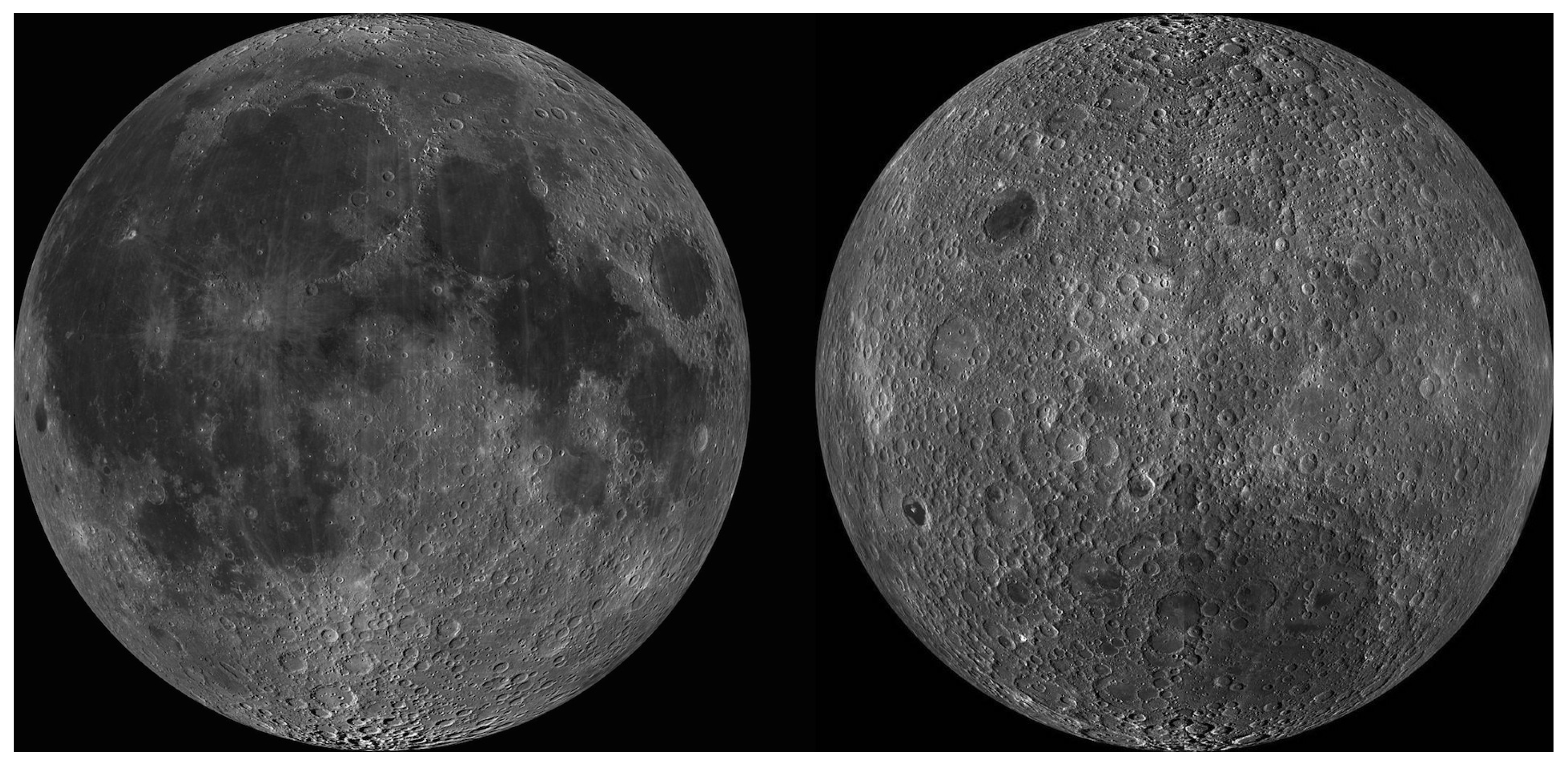
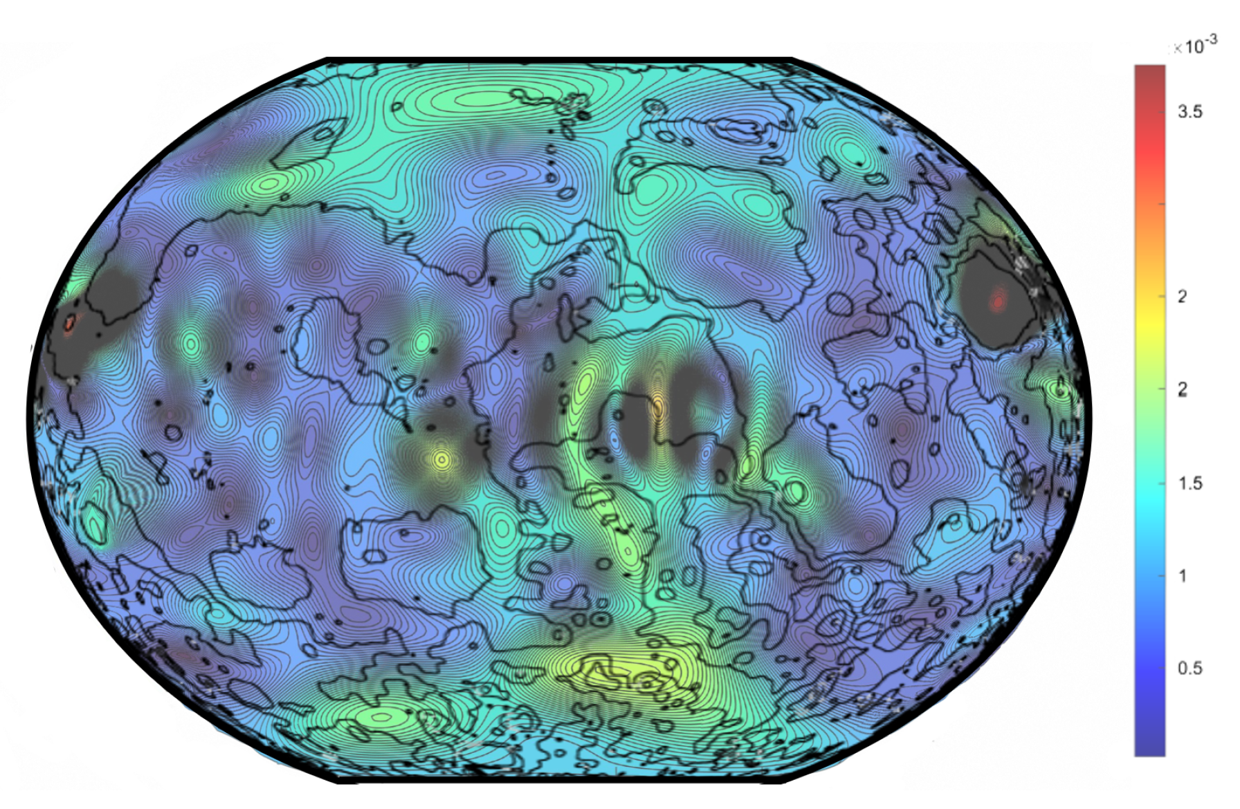
Figure 1.
Left: The Moon’s near side. Right: The Moon’s far side. Image credit: [
1].
Figure 1.
Left: The Moon’s near side. Right: The Moon’s far side. Image credit: [
1].
On March 4, 2022, at approximately 4:25 a.m. PST, a rocket component was reported to have crashed into the far side of the Moon [
2]. Although the specific rocket component is still not verified, losing control over spacecraft during lunar orbit missions has been an ongoing issue since the launch of the Luna 1 rover in 1959. Moreover, scientists have noticed a peculiar phenomenon about the lunar surface gravity: as satellites and probes orbited the Moon over certain craters and impact basins, they periodically veered off course and sometimes even plummeted toward the lunar surface. This is a particular problem when observing these effects on the far side of the Moon (See Fig. 1). It wasn’t until the Apollo 15 and 16 missions that scientists described the Moon’s surface gravity as “lumpy” due to the differing mass concentrations caused by the geology. These fluctuations in the lunar surface gravity have always puzzled scientists, which led to a high demand for precise lunar gravity data in the hopes of avoiding these crashes.
From the Lunar Reconnaissance Orbiter (LRO) [
3] to the recent Artemis program [
4], the field of lunar-based orbit propagation research has been increasingly growing over the decades. As a result of this, the importance of modeling the lunar surface gravity anomaly to aid in future Moon missions has become crucial in predicting the trajectories of spacecraft orbiting around the lunar surface. Using high-resolution gravity data, many lunar surface gravity models, such as NASA’s Gravity Recovery and Interior Laboratory’s (GRAIL) GRGM1200B model [
5] and the GSFC LP-100k lunar potential Model [
6], have been created as an attempt to constrain lunar surface gravity anomalies in response to this demand. Although sufficient enough to model the lunar surface gravity, these existing models rely on the global spherical harmonic (SH) series to solve Laplace’s equation for gravity. The SH method for solving the equation of gravity was initially implemented as a way to model the geopotential through the use of Earth-based satellites recognized in the late 1950s [
7]. Recent projects that implement gravitational acceleration modeling about the Moon can be viewed in the following literature: [
8,
9], and [
10]. However, the SH approach proves to be computationally demanding, with three main issues arising: [
11,
12,
13]:
At polynomial orders , convergence proves to be inefficient and slow, which requires tens of thousands of terms to obtain accuracy for higher-order gravity representation.
In any astronomical surface gravity modeling, the north and south poles represent singularities in SH which result in poor approximations at the poles. For further examinations on obstacles in SH gravity approximations [
14,
15,
16]
SH is only accurate with spherical-shaped astronomical bodies. This means that the gravity of objects such as comets and oblate bodies cannot be modeled using this method.
We hope to introduce a FEM local gravity representation of the higher order perturbation to offset the issue of slow convergence of the gravity models at polynomial orders greater than 2. Specifically, we hope to use lower-order functions to sufficiently model the gravity perturbations about the lunar surface. This is highly motivated by literature where the projects propose similar advancements to the classical SH approach, such as in Junkins [
17] and, more importantly, in recent investigations by the following: [
18,
19,
20].
This paper details a new approach to modeling surface gravity anomaly, increasing computational speed while maintaining a conservative error. Specifically, we propose replacing the current LP-100k lunar SH gravity model with a series of local orthogonal polynomial approximations implemented by the Finite Element Method (FEM) of modeling lunar surface gravity. In Bani Younes’s dissertation [
21], a FEM surface gravity model was implemented for the geopotential, which holds significant relevance to our applications on the lunar FEM model. With this paper, steps have been taken to produce a cost-effective and accurate FEM lunar surface gravity model that will mirror that of the dissertation. Furthermore, parallelization of the lunar FEM surface model will be implemented building upon the research of [
22] where a parallel evaluation of Chebyshev approximation was studied. Parallelization of the original FEM lunar model and astrodynamics applications using the FEM model will further encourage computational speedup in both regards. With this, creating a FEM lunar surface gravity model will elevate the surface gravity modeling field with these main contributions:
Computational efficiency
Memory allocation
Precision
Parallelization
1.1. Finite Element Method
There have been a variety of approximation techniques and basis functions implemented for gravity representation which includes weighted functions [
12,
23,
24], wavelets [
25], splines [
26], octrees [
27], psuedocenters [
28] and 3D digital modeling [
29]. FEM can be used in a wide variety of applications that are both interesting and important in the fields of mathematical modeling, engineering, and computational analysis. Some examples include using FEM to analyze electric sail static structures [
30], determination of the gravity potential and tidal stresses of asteroids [
31], and using FEM to analyze a lunar lander during a soft landing [
32]. Similar to our approach, each method balances accuracy with efforts to encourage computational speed. FEM was first proposed by Junkins [
17] as a way to interpolate the geopotential of Earth-based gravitational modeling. Bani Younes [
21] provided the computational framework to implement FEM to model the geopotential, acceleration due to gravity, and radial adaption about the Earth’s surface. With this descent, the purpose of this paper is to interpolate the lunar gravitational acceleration about the surface and above the surface to help aid future lunar-based spacecraft missions that require precise orbital propagation.
Using the lunar FEM model, truncating the classical expansion at will allow for local gravity representation at the higher-order perturbations. The FEM modeling approach is applicable to any spherical model and even to irregularly shaped astronomical bodies, while SH is purely for spherical bodies. Furthermore, this method increases computation by trading computer memory for run-time speed.
For our purposes, FEM will be used on the lunar surface, where the method will subdivide the entire lunar surface as a large system and subdivide it into smaller finite elements. The gravitational differential equations will then be solved in each shell and will then be connected by nodes. However, determining the correct shell iteration for these higher-order approximations is key with this method.
1.2. Chebyshev Polynomial Interpolation
Developing a more efficient theory to solve higher-order Laplace’s equation for gravity requires a structure that is both radially adaptive and efficient. If implemented correctly, interpolation at any radial or point on the surface can be made. One approach involves using the Chebyshev polynomial method. Created by mathematician Pafnuty Chebyshev in the nineteenth century, Chebyshev polynomials are two sequences of polynomials related to the cosine and sine functions denoted as and , respectively. The polynomials can be defined starting with trigonometric functions where:
The Chebyshev polynomials of the first kind (
) are given by:
and the polynomials of the second kind (
) are:
in which
n is any integer number that can be used to convert these definitions into a polynomial form. Chebyshev polynomials are orthogonal polynomials that are solutions of a special kind of Sturm-Liouville differential equation called a Chebyshev differential equation. Most importantly, the roots of
i.e. the Chebyshev nodes, are used as estimation points. Approximating at this point produces efficient polynomial interpolation, which is useful for precise radial adaptation and other applications which require higher-order approximation.
Although typically used as a numerical method for solving initial value problems (IVPs) and certain classes of boundary value problems (BVPs), this method can also be used to approximate solutions of linear or non-linear ordinary differential equations (ODEs) like that of Laplace’s equations for gravity. Using these Chebyshev polynomials, an orthogonal approximation can be placed for our FEM modeling process in which the path approximations would encourage computational speedup.
1.3. Orbit Propagation
The last application in this project includes using the FEM model to approximate a satellite’s orbital trajectory over a provided time span. Similar works which inspired this method of orbital propagation can be found in the following literature: [
33,
34,
35]. This application will be achieved using the resulting Chebyshev polynomial coefficients from the original FEM routine at specific radii above the lunar surface to approximate the acceleration a satellite with negligible mass would experience during the course of a short and long-term orbit around the Moon. This propagation considers the two-body problem, which consists of a satellite with negligible mass orbiting a larger astronomical body. This problem allows us to use Newton’s second law force equations to then come up with a finalized two-body equation of motion for the theoretical satellite orbiting the Moon. In this paper, we will first cover in detail the orthogonal approximation techniques used alongside Chebyshev polynomials in Section II. Then in Section III, the process of utilizing FEM on the LP-100k model will be discussed and compared to the original SH model. In Section IV, we will discuss how we implemented the coefficients produced by the FEM model on a two-body orbit propagation problem about the lunar surface. Lastly, in Section V, we will discuss a summary of the finding and concluding remarks.
2. Orthogonal Approximation
The following are some examples of treatments of discrete approximation using Chebyshev polynomials: [
24,
36,
37,
38,
39,
40,
41,
42,
43]. Although [
39,
40] hold more significance in the field of orthogonal approximation, in [
42], the orthogonal approximation is used to show that multi-resolution approximation of input and output maps can be linear and nonlinear. Typically, a linear least-squares approximation is used for an orthogonal approximation when dealing with experimental data or an arbitrary function generating polynomials. In this paper, a least-squares approximation with classical Chebyshev polynomials is used to analyze discrete samples of the “to-be” approximated function. Furthermore, arranging the regression matrix to be “Kronecker factorable” (a technique used in [
21]) allows the use of array algebra identities to generate the multidimensional orthogonal least-squares operators. This approach can be seamlessly adapted to higher-dimensional approximations. This section summarizes how using the Kronecker product technique extends a single classical Chebyshev polynomial approximation result to higher dimensions. This method avoids dimensional challenges related to how many attributes a dataset has and paves the way for efficient computation. The importance of this method allows considering the advantages of orthogonal approximation in gravity modeling. Most mathematical derivations are based on the work presented in [
21].
First, let’s briefly consider the following approximation of a single-valued function,
, with
x as one independent variable:
For simplification in multi-dimensional analysis, we introduce a new independent variable
where
. Thus, through the process of normalization, the forward and inverse transformation for
can be produced:
The final function to be approximated can be created by substituting the forward and inverse functions into equation 3:
In a general case, for basis functions,
, we seek to approximate
as a linear combination of a set of
linearly independent basis functions
as the following:
For discrete cases, we introduce a set of sample points in which we call
nodes as
. With this, we can consider the residual approximation error at each node to be:
In general, the decision to use a least-squares approximation routine is motivated by the advantages of applying the one-dimensional analysis to higher dimensions. This motivation is discussed later in Section 2.4. Using least-squares approximation, we want to find the coefficient vector
a that minimizes the weighted sum square of the residuals:
where
, and
W is a positive definite weighted matrix determined by classical orthogonal conditions for Chebyshev polynomials (see Section 2.2).
Using a weighted least-squares solution and orthogonal conditions, this result can be displayed as normal equations:
This finalized relationship can be displayed in matrix form as the following:
Similarly, for more than one independent variable, we can consider the function
, with the two independent variables
x and
y:
as in our one variable approximation example, we will use a set of new independent variables,
, and
, to reduce the computational burden of dimensionality which leads to the normalized forward and inverse functions:
Substituting these equations into equation 11 provides us with the function we wish to approximate:
and in the discrete measurement case tested at sample nodes,
,
, the residual approximation error at each node is:
Which can be displayed in vector-matrix notation:
where
. When in matrix form, a common issue that needs to be considered is dimensionality. To avoid this problem, efficient choices of basis functions and associated sample points must be made. This technique is examplified in [
44]. Referring to sections 1.6.2,
is formed as the Kronecker product of two basic matrices:
For our purposes, the Kronecker product,
will be implemented in MATLAB [
45] via the “kron” command. Subsequently, our weighted least-square solution matrix becomes:
As equation 2.19 is “Kronecker favorable”, it can be further represented as
. Furthermore, this result can be generalized to higher dimensions as the following:
which allows for us to generalize Eq. 2.19 into a three-dimensional approximation space
or
:
Using the Kronecker product of three small least-squares operators to produce a larger operator allows us to approximate in higher dimensions by taking the cube root of the size of the three inverted matrices. Going up dimensions would require us only to introduce a fourth variable, which is the beauty of this Kronecker product trick. See the Appendix for more details about the properties of the Kronecker product and how lower dimensional analysis can be easily “upgraded” to higher dimensions. With this, we can generalize the above equation to
n-dimensions by taking the
root of the inverted matrix dimension:
where
C is the Cholesky square root of
of the weighted matrix
. and
,
which makes
Kronecker factorable. This final result allows the same advantages to be used in the identity-weighted matrix case. With this, equation 2.20 can be expressed as:
where
,
,
,
, and
.
It is useful to note that
and
have a Kronecker relationship:
which allows for us to sample locations corresponding to the Chebyshev polynomials. The Kronecker product trick for constructing the two-dimensional Chebyshev least-squares matrix can be provided by:
where
. The most important takeaway from this step is that
C is also Kronecker factorable, just as our weighted matrices
W is. From the above conclusions, we can finally apply this formulation to
n-dimensions. Take the following example for approximating a function in three dimensions:
For our final generalized function, consider a function of
n independent variables:
with the following forward and inverse functions:
We can then write the function we wish to approximate by substituting Eqs. 2.26 into 2.25 using our independent variable (as we’ve done before):
Similarly, for discrete measurements, we introduce a set of sample points (nodes):
. This produces the following residual approximation error at each measurement node:
where the
k indices represent the measurement for the
variable. Equation 2.28 can written in vector-matrix notation,
. Finally, as mentioned in our two and three-dimensional examples, the weighted least-squares solution can be written as the Kronecker product of
n smaller least-squares matrices:
where
,
, and
, and
.
To conclude this section, it is good to note that the previously discussed methods of orthogonal approximation, i.e. the use of least-squares approximation with Chebyshev polynomials alongside the Kronecker product trick, will be implemented in our FEM approximation routine, specifically for the three-dimensional case in approximating Laplace’s gravitational differential equations.
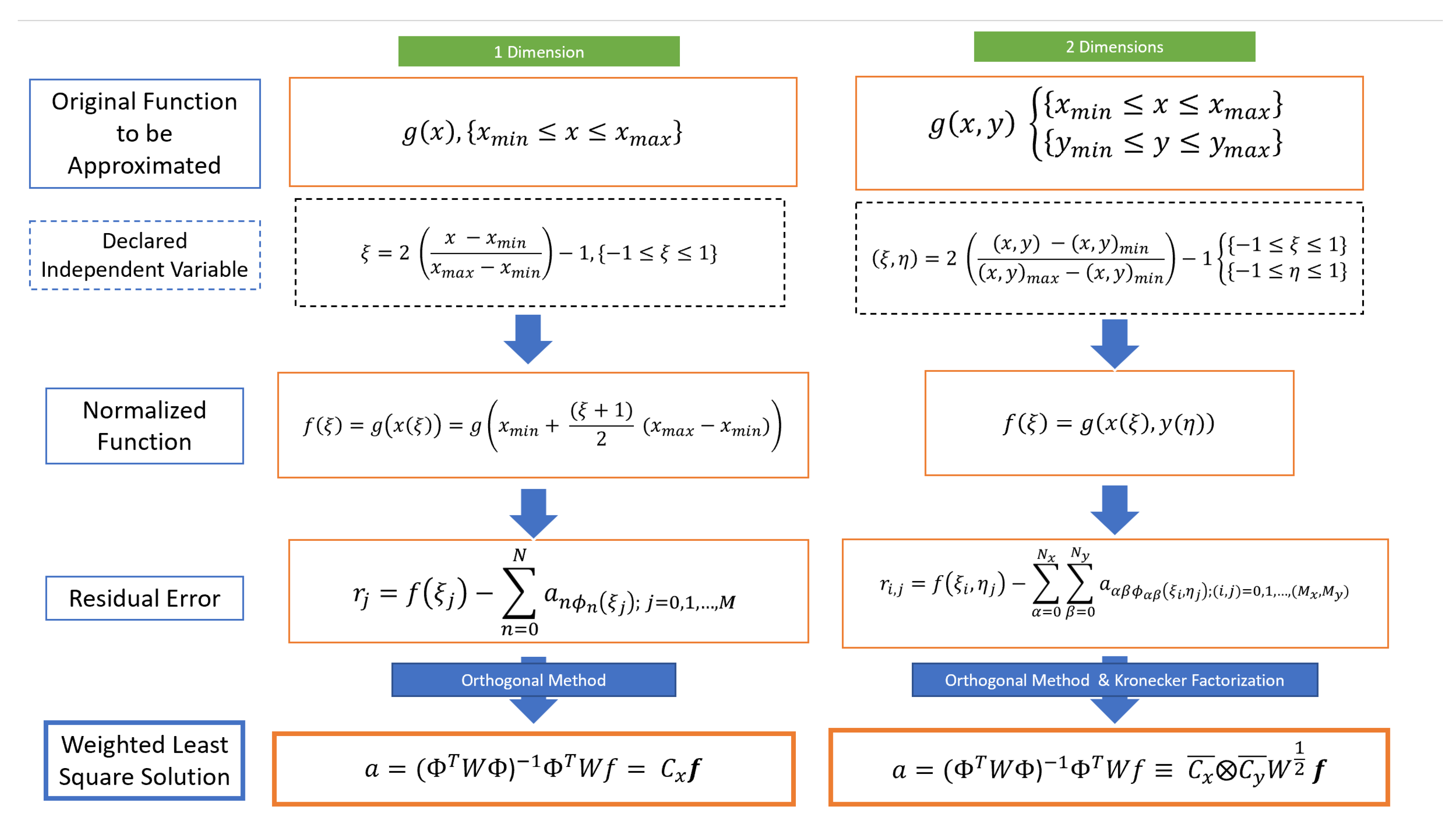
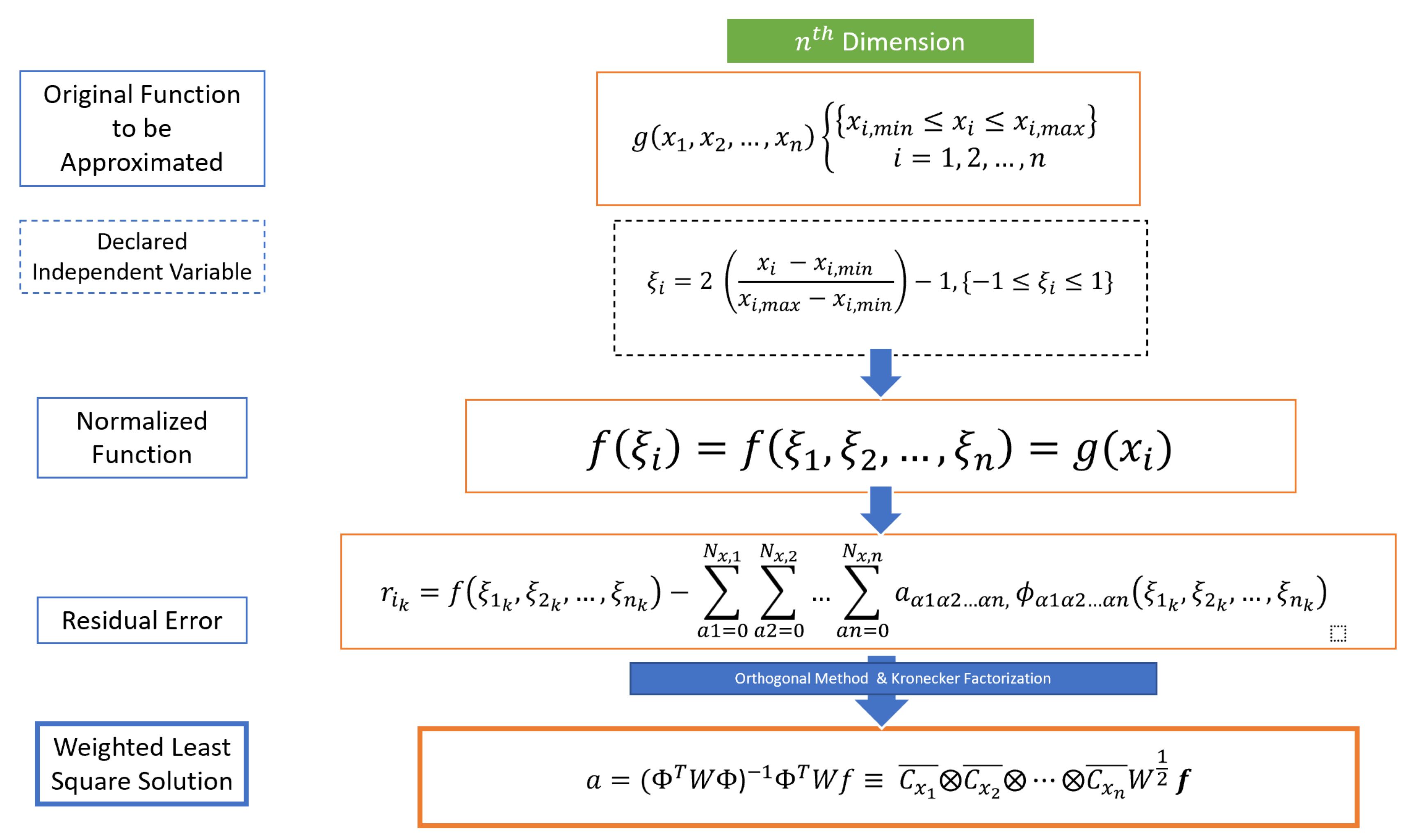
Figure 2 and
Figure 3 summarize the steps taken in our approximation routine for the one, two, and
n-dimension approximation routine.
3. Representations of Lunar Potential Using Orthogonal Finite Elements
In the following discussion, we consider a basic orthogonal FEM approximation to a gravitational acceleration model determined from NASA’s lunar Prospector (LP) mission in 100 spherical harmonic degrees [
46]. Released in 2000, the LP Gravity model allows considerations of an analogous FEM approximation of the ‘LP100K’ gravity model. For high-precision orbit propagation, we consider all terms used in the
LP model. Using this model, we solve Laplace’s equation for gravity using FEM and compare it to the classical spherical harmonic approximations. Initially, a test was done to produce a contour plot of the disturbance gravity acceleration on a small degree order using our FEM approach. This test ensured a reasonable error value on top of a reasonable computation time which encouraged us to continue the procedure with a higher degree order for an accurate representation.
Figure 4 shows the radial disturbance acceleration on the lunar surface from our FEM representation with
degree square using
approximation.
As mentioned in the introduction, the three main challenges faced when using SH for orthogonal approximations are 1) An upper limit discrepancy, 2) inefficiency at orders higher than 2, and 3) Non-free singularities at the poles of the astronomical bodies. With these three challenges in mind, we introduce a Finite Element Method (FEM) model of surface gravity representations in the hopes that lower degree functions produced can be implemented to effectively and sufficiently model and compute lunar gravity. Furthermore, this method can be parallelized to increase computational efficiency. With this, we have to structure the FEM model to be both radially adaptive and efficient, which will result in better interpolation at higher degrees (i.e. at different radial distances above the surface of the Moon).
We will be considering the following gravitational potential model that is made up of the reference and disturbance gravity terms where the reference term includes two-body effects on the lunar gravity (
) while the disturbance term (
) includes any other effects on gravity for the higher degree and order terms to take place. With these two terms, the finalized potential,
can be given as:
Furthermore, the acceleration can be derived from the potential and is represented as:
It is important to note that adjusting the model to correct for the two-body interference will be done before we can consider the reference potential compact and efficient. This means only the perturbing acceleration terms are considered in our model.
3.1. Sampling: Radii and Shells
To help illustrate a sample FEM grid, consider a spherical grid with radius (i.e. a sphere with the radius of the Moon at the lunar equator). This sphere is then covered by a 2-D mesh from and . It is good to note that the poles are neglected in this routine due to the limitations of the original SH model. As discussed, the poles of astronomical bodies are treated as singularities in SH modeling. However, the FEM model can be used to approximate the surface gravity at the poles using the Cartesian coordinates. This will be implemented in later approximation models. The following section will allow us to discuss the process of finding the most efficient initial conditions like shell size and radius sample.
3.1.1. Radial Sampling
At an arbitrary radius, r between , let the gravity data be provided at a constant radius, r, on a specific spherical shell. This data on this shell should be transformed into , where and , we can retrieve an accurate gravity modeling representation of on “sufficiently-dense” sets of concentric spherical surfaces. However, sampling radial coordinates is key when considering this unique variation.
To determine a proper radial sample, we consider two different sampling methods:
uniform sampling, where we approximate the gravity at every radii between the lunar surface to 200 km above in 10 km increments, and cosine sampling. For
cosine sampling, consider the transformed position
r in which the position follows a “cosine-like” transformation as a function of the previously mentioned variable
as the following:
where
where
and
,
and
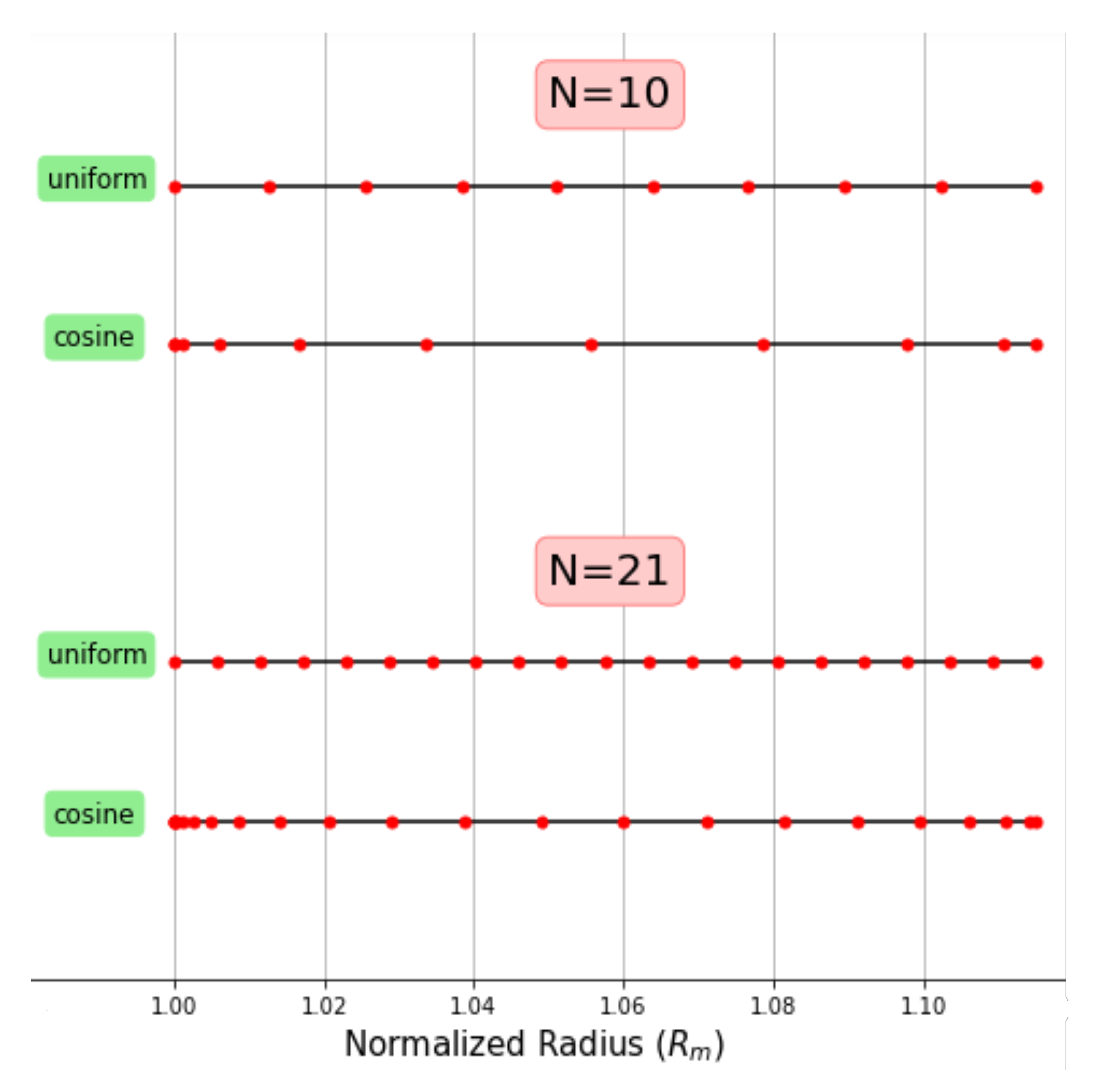
. At higher radii above the lunar surface, gravity anomalies decline rapidly. With this fact, we seek to format an efficient way to sample surface gravity that allows memory allocation. With cosine sampling, this transformation “naturally” constraints dense measurements at smaller radii ensuring that gravity perturbations are maximized and mimic how gravity would naturally act. This means that no matter the number of points
N at lower radii, these nodes then bunch up in comparison to larger radii. This idea is illustrated in
Figure 5 for 10 and 21 sample points as we compare this method to uniform sampling. To compact this progression, the transformed radius variable
was created to help treat
r as an independent variable. It is again important to note that
is sampled non-uniformly using another cosine transformation in order to satisfy the Chebyshev orthogonality conditions:
Not only does cosine sampling simulate a natural progression in gravity, but this sampling method also produces the error magnitude on the order of () while taking the same amount of computational power as uniform sampling. For these reasons, we will continue using cosine sampling in our analysis at a latitude and longitude of = = degrees on the Moon.
3.1.2. Shells and Polynomial Order
After determining a proper radial sample, determining the required polynomial order as a function of radius is the next step. We want to determine this order that adaptively maintains an efficient error tolerance. The required acceleration error tolerance is determined from the polynomial order N at every radius. For example, if we consider a 4-by-4-degree square area on the lunar surface, the convergence error is the maximum absolute error between the LP SH model’s acceleration values and the approximated acceleration from our method.
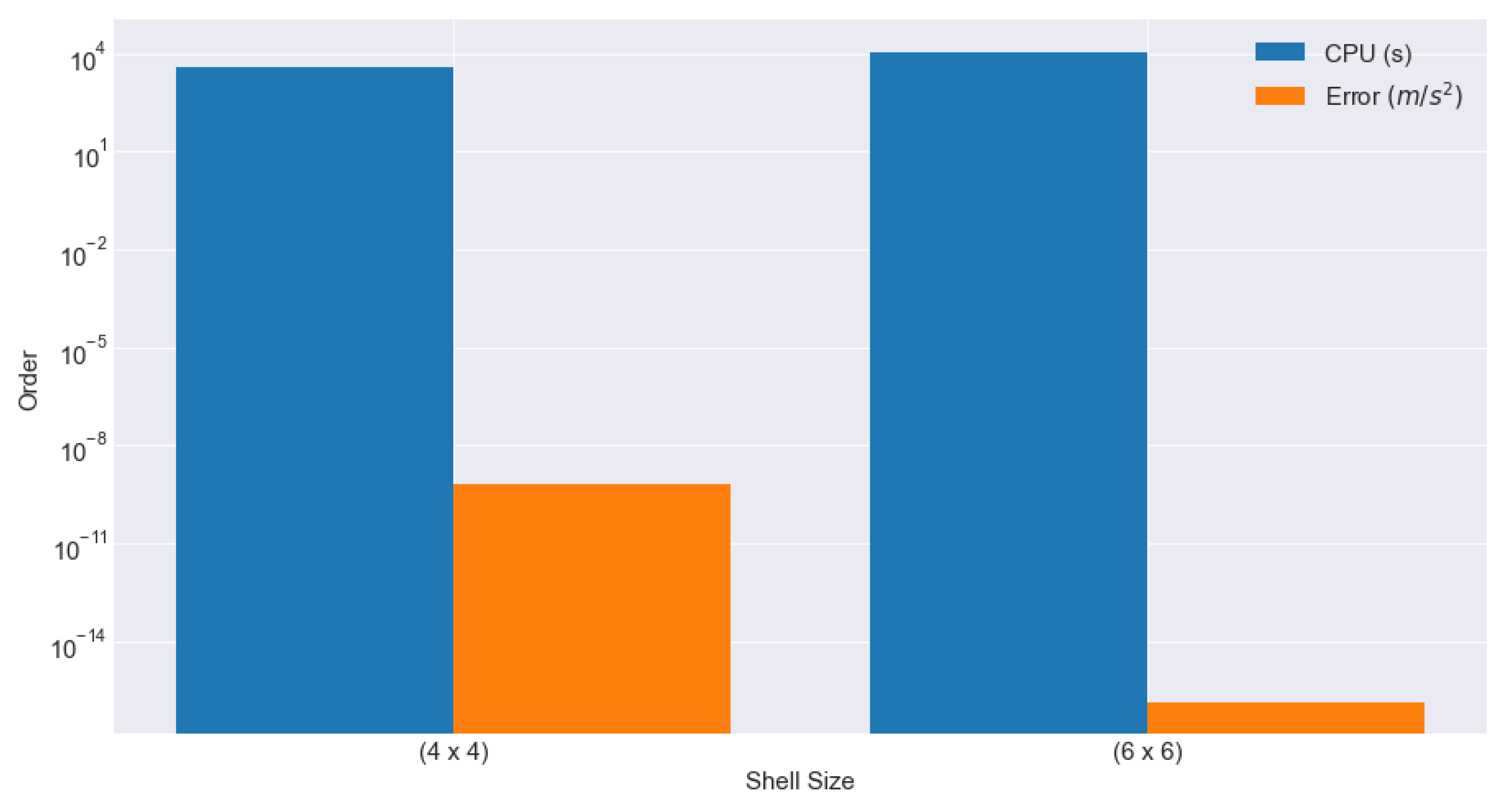
Consider a shell size of square degrees compared to a smaller size of square degrees. The shell size would require less computational power/time to compute all the coefficients over a small area, while the shell size would require a longer computational time to reach a similar error tolerance because of the larger number of coefficient values calculated. The compromise of time would be better justified with the resulting error produced. Although the larger shell size may take a longer period of time to produce results, if these results display a small error tolerance (), it would be best to use this. Thus, when determining the correct shell size for our model, we want to pursue a shell size that maintains an efficient error tolerance while not compromising computational power.
With a maximum degree order of 100 and shell sizes of (
and
, we evaluated both sizes and checked for accuracy and computational time across a portion of the near side of the lunar surface (from
and
). As discussed previously, the smaller shell size of
would be more desirable if the computational time is reasonable. However, if the accuracy for the
case is reasonable compared to the
shell case, this shell size will be considered.
Figure 5 displays a graph of computational time and calculation error as a function of shell size. For a shell size of
as maximum degree order of 100, it took the machine (see machine configurations in Section V) approximately 3627.43 seconds to produce the relevant FEM approximation coefficients with an error of
. For the
case, it took the same machine approximately 10653.11 seconds to produce the FEM approximation coefficients with an error of
. With the shell size of
providing such a small error compared to typical errors found in other FEM surface gravity models produced in [
21], we found that this error is insignificantly smaller given the increased computational time. With this, we have concluded that the
case provides the best balance between computational time and reasonable accuracy.
Figure 6.
Comparison between shell sizes of and square degrees.
Figure 6.
Comparison between shell sizes of and square degrees.
3.2. Orthogonal Approximation of the Gravitational Acceleration
Using orthogonal approximation, we estimated the lunar gravitational acceleration by transforming gravity into sample points. These sample points are located in our distribution in the least-squares approximation. In this subsection, we will briefly discuss our approach.
Let gravity data
transform to
with sample points located as a cosine distribution. For the three components of gravity, the approximation is as follows:
where the indices
range from 0 to
, and
are the basis functions (which are transposed) of the acceleration components.
Furthermore, Equation 32 can be expressed more compactly if the same basis function for the acceleration components by using
=
=
=
which provides us with the following relation:
. We then utilize the tensor product of
and the identity matrix,
, twice to “undo” the transpose acceleration components. This creates the finalized gravitational acceleration approximation equation:
To use the FEM for computing gravitational acceleration, we employ the maximum polynomial order, ensuring consistency levels as compared to the overall model. In particular, at larger radii above the lunar surface, the computational speed decreases by an order of magnitude when only non-zero terms are included.
3.2.1. Parallelization
Recent developments have seen the parallelization of gravitational FEM models, as implemented in [
22], utilizing the Open Multi-Processing (OpenMP) application interface, which supports shared-memory parallel programming in C/C++ and Fortran. In this project, the inputs are the spherical coordinates (
) with corresponding normalized parameters
,
, and
which are used to evaluate the Chebyshev polynomials. The master thread is then split into slave threads, each evaluating the multivariate Chebyshev polynomials in parallel. These threads are then joined back together to be evaluated for the FEM acceleration by adding spherical and
terms. A three-magnitude speedup was reported using OpenMP on a geopotential FEM model with 8 threads. Even with a more efficient computation time, the parallelized FEM model still produced less than 10 digits of accuracy compared to the original SH model. With this in mind, OpenMP implementation to the FEM lunar model promises higher speedup gains if more threads are used. This study indicates potential efficiency gains in both memory allocation and computation time for future FEM lunar model developments.
3.3. Results of the FEM LP Analysis
The following discussion delves into the results derived from the above-mentioned FEM routine applied NASA’s LP100K SH model. The primary focus is on determining the best parameters for achieving an optimal balance between computational efficiency and error minimization.
For cosine sampling, the number of CGL nodes was highest near the surface and would decrease as the radii increased. The number of sample nodes should decrease as nodes are related to the number of coefficients used in the polynomial approximation at a specific radius. In order to find the best node quantity for each radius, we iterate our routine through uniform node values at each radius until a node value produces an error greater than a tolerance of
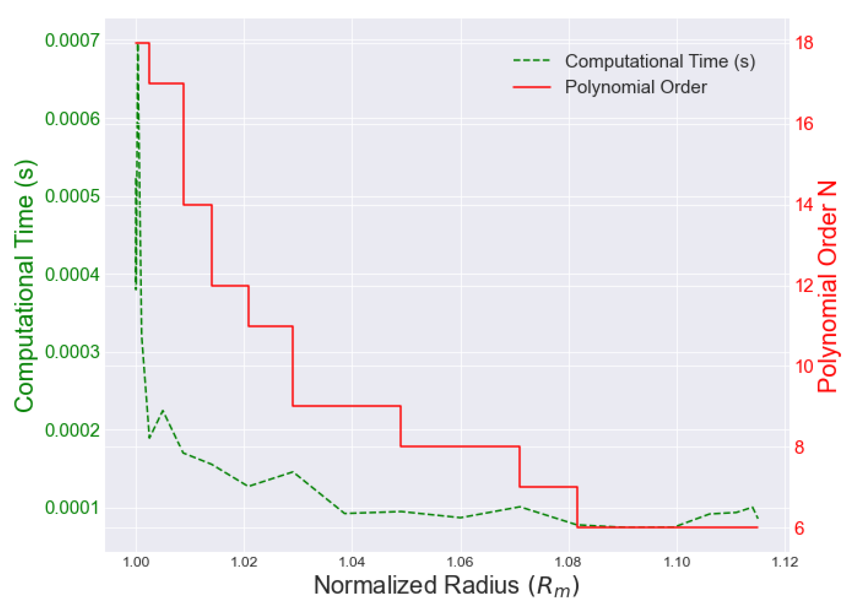
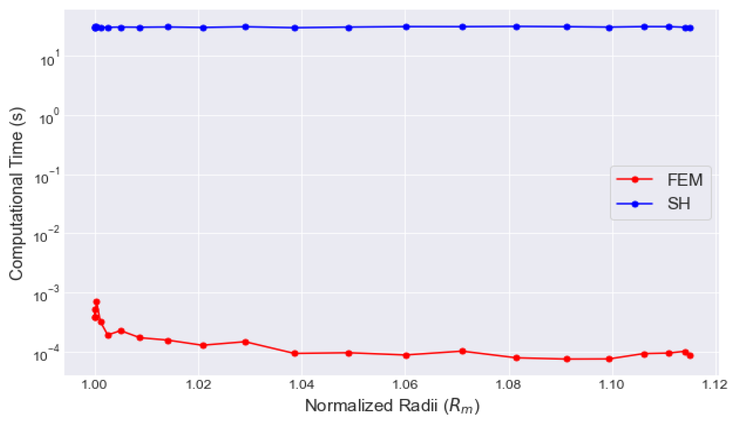
. Because the number of CGL nodes is related to the polynomial order, we want to further our investigation by observing how the polynomial order affects computational time. With this, we find an analogous relationship between CPU time and polynomial order (as expected).
Figure 7 illustrates a decrease in time cost as a function of radius alongside of the polynomial order decreasing in the same manner confirming the idea that it takes a longer period of time to approximate at higher polynomial orders than at lower orders.
For higher precision orbit propagation, we consider all terms used in the
LP spherical harmonic model. As mentioned in our approximation theory, we select an error tolerance of
while substituting the high-degree order gravity model with a FEM approximation.
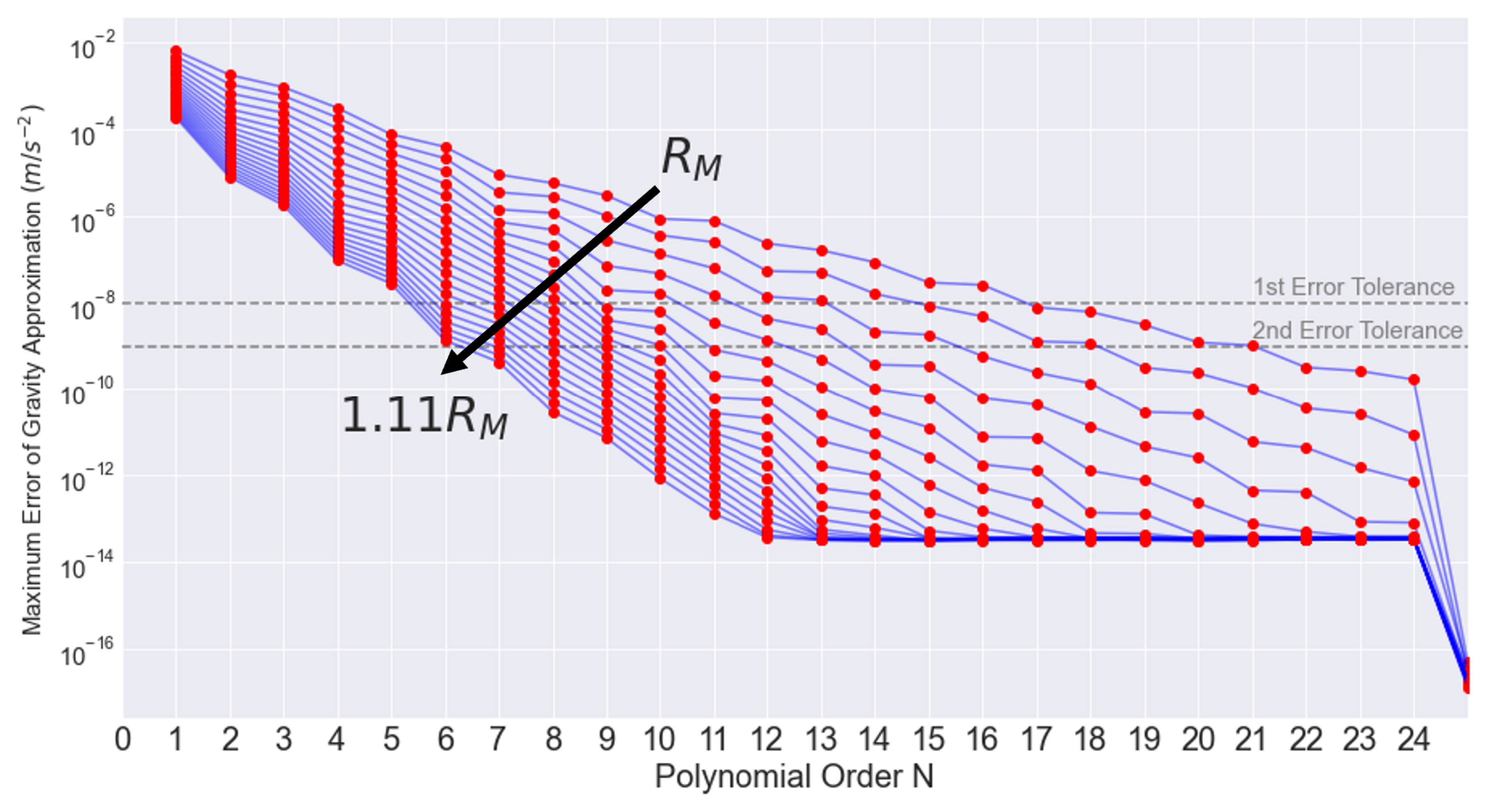
Figure 8 showcases the maximum absolute error of the approximated norm of the “disturbance” acceleration as a function of the Chebyshev polynomial order
N. Here, we note that as the radius increases, the error declines faster; a smaller polynomial order is sufficient enough to reach the placed error tolerance of
. However, in this plot, we can see that there are two error tolerance values displayed. In our previous analysis, we identified a polynomial order of 21 that yielded an error of
. However, after reviewing the coefficient values in this polynomial order, we found that the portion of corresponding errors was much smaller than our allowed error tolerance. This suggests that this polynomial order was significantly implementing a high precision that was computationally expensive. With this, we implemented a “fetching” routine where any error values less than our error tolerance had their corresponding coefficient value to be approximated to 0.
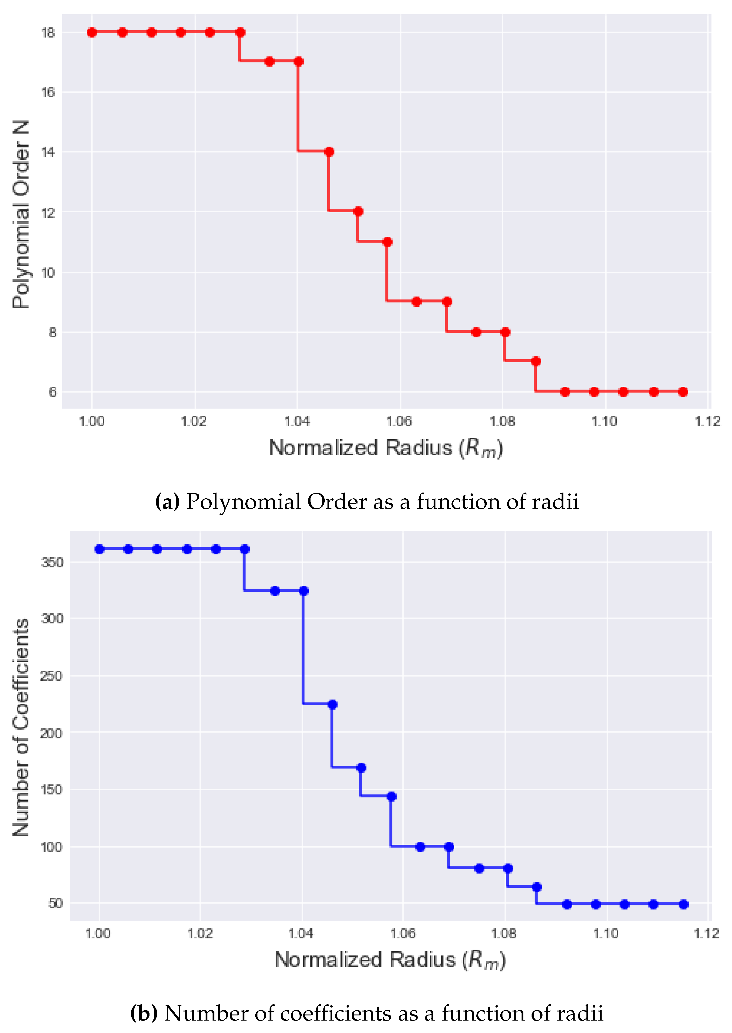
As an outcome, most of the coefficient values were approximated to 0, further suggesting an excessive polynomial order. After revisiting our analysis and the polynomial order of 18 was found for the surface, the same “fetching” routine was done with , finding that none of the error values strayed too far past the error tolerance, which was apparent in the weight of non-zero coefficient values found in that sample. This led us to believe that a maximum polynomial order of 18 was the most reasonable (computationally supportive and precise) option for the surface of the Moon. An error tolerance of proved to be too conservative. With this, a more liberal error tolerance value of was placed to ease the amount of computational burden while also still maintaining reasonable error.
As we get closer to the surface of the Moon, a higher polynomial order is required to reach this error tolerance. The (100, 100) LP model’s gravitational acceleration values are used as the truth and the errors between the FEM approximation are reduced by adjusting the degree value of the Chebyshev polynomials until it reaches the error tolerance. For our lunar model, we found that the most efficient maximum approximation error is which provides a fair balance between computational time and machine precision at a maximum polynomial order of N = 18 on the lunar surface with a square degree FEM cell size. However, when a polynomial order of 18 was applied to a radius 100 km above the lunar surface, we find that the error produced is negligible. This confirmed our previous discovery about a decreasing radial polynomial order i.e. as you go further from the surface, the polynomial order required to reach the error tolerance decreases as well. Furthermore, a Maximum degree value (M) of 100 and a shell value of degree maintains an efficient error tolerance while constraining sensible computational power.
The determination of the correct polynomial order for each radial adaptation allowed for us to determine the number of coefficients required in approximation at each radius. At the lunar surface, the polynomial order of
indicates that the gravity acceleration at the lunar surface can be approximated by
orthogonal polynomial terms (or coefficients). At 200 km above the surface, a polynomial order of
was found to be most efficient, which means it requires 49 coefficient terms. This suggests that as the polynomial order increases, the number of coefficients required in the approximation also increases as well. This relationship can also be supported when observing how an error is related to the node number at each radius.
Figure 9 displays two plots; (a) polynomial order as a function of radius and (b) number of coefficients as a function of radius; these plots show a nearly similar result.
On the same machine, the FEM model displays three orders of magnitude of computational speedup at the lunar surface compared to the (100, 100) LP SH model. This can be seen in
Figure 10. As we approach this comparison radially, the FEM approach continues to be computationally efficient compared to the original (100, 100) SH model, even going as far as to decrease computational time as it reaches higher radii. At radii
R near
, we find that the FEM approaches five orders of magnitude of computational efficiency compared to the SH model. If implemented for orbit propagation, the FEM gravity model should not only provide a 9 to 10-digit of accuracy, but it will also produce a 3-5 order of magnitude reduction in CPU time.
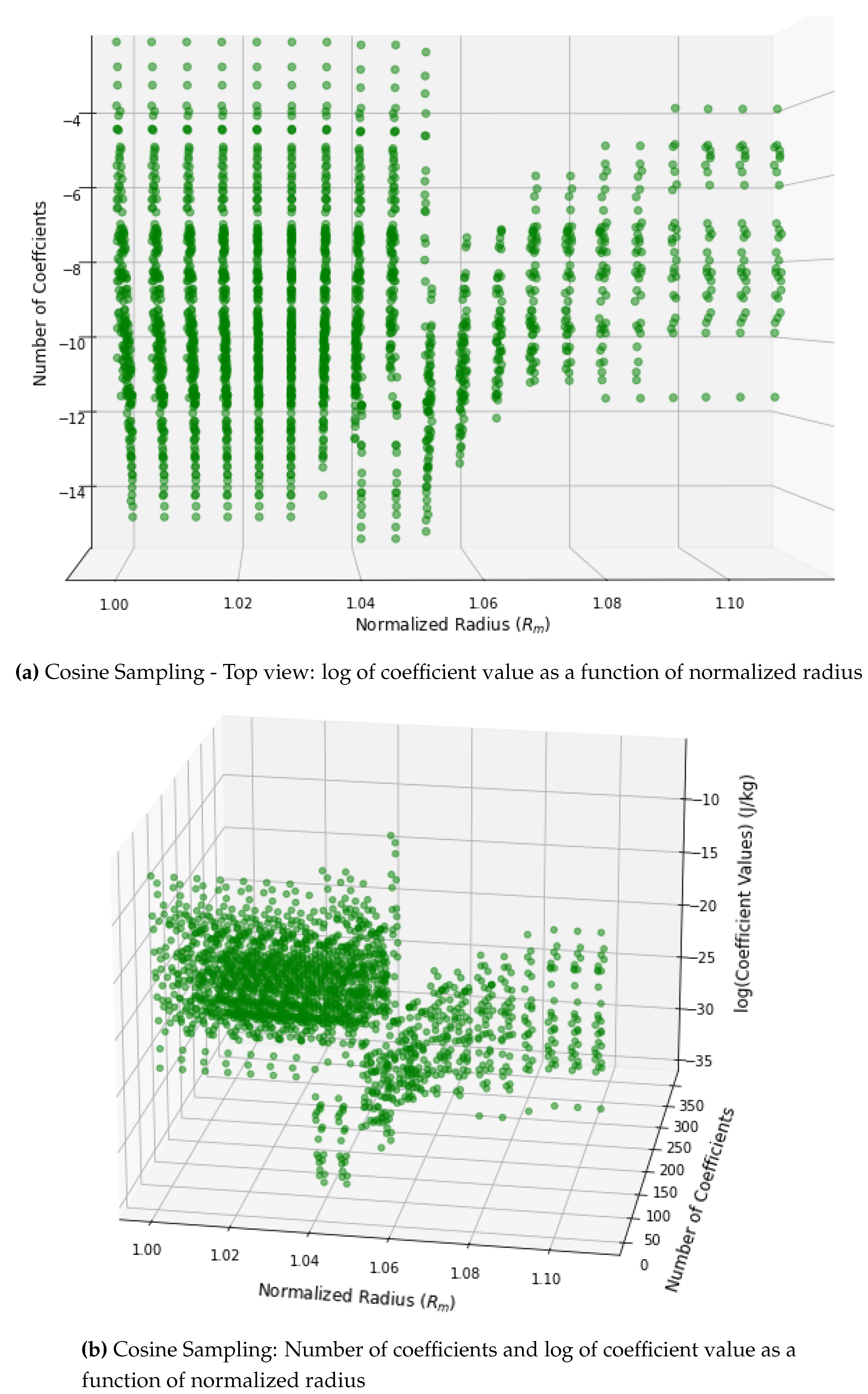
The Chebyshev coefficients were saved for each radial iteration. These first 49 coefficient terms are displayed for our final cosine sampling
Figure 13. With cosine sampling, higher-order non-zero coefficients have been found to be comparable to easy-to-fit smooth functions of similar nature. With this, it is observed that the norm of gravity decays rapidly, as it should.
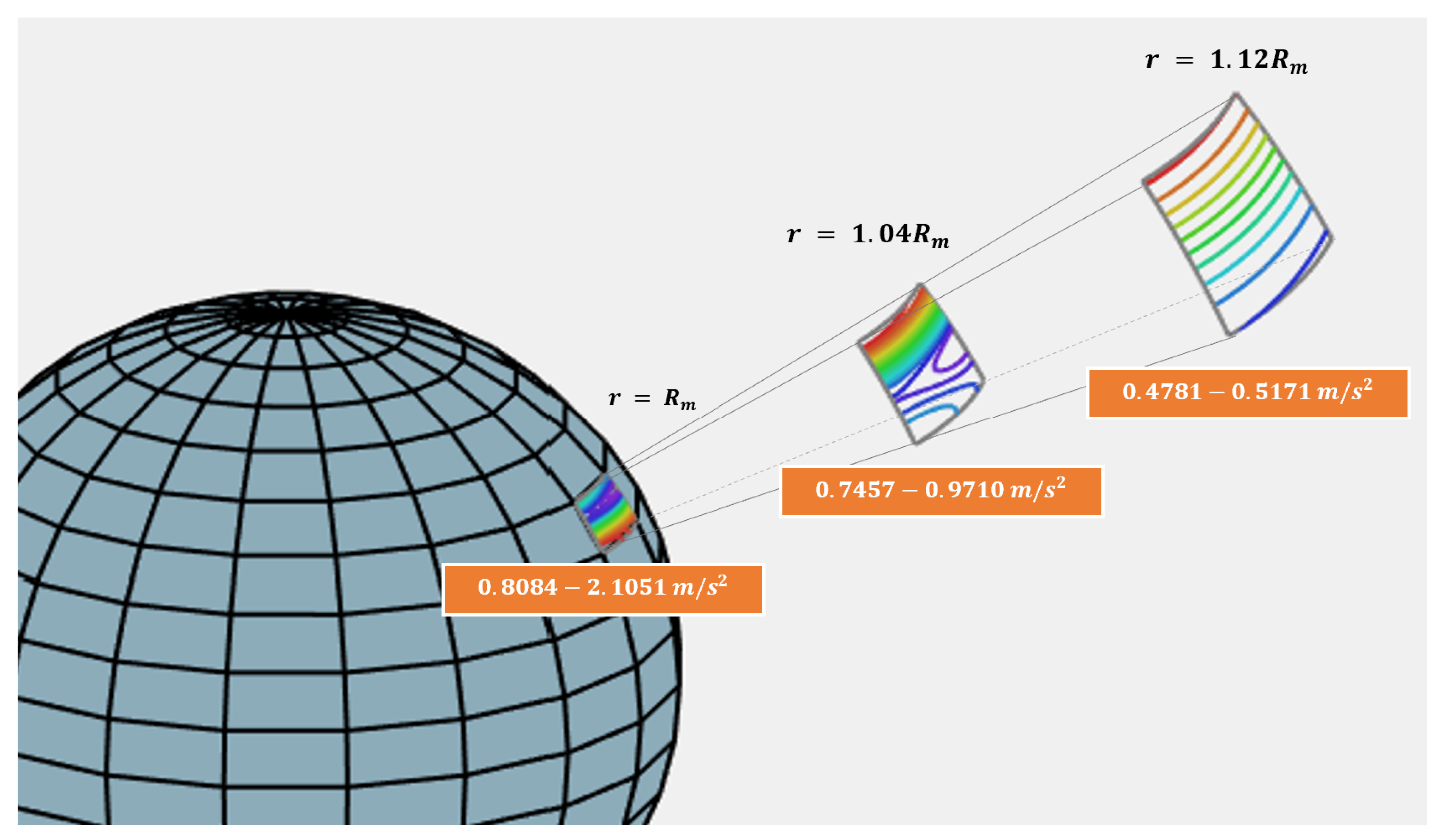
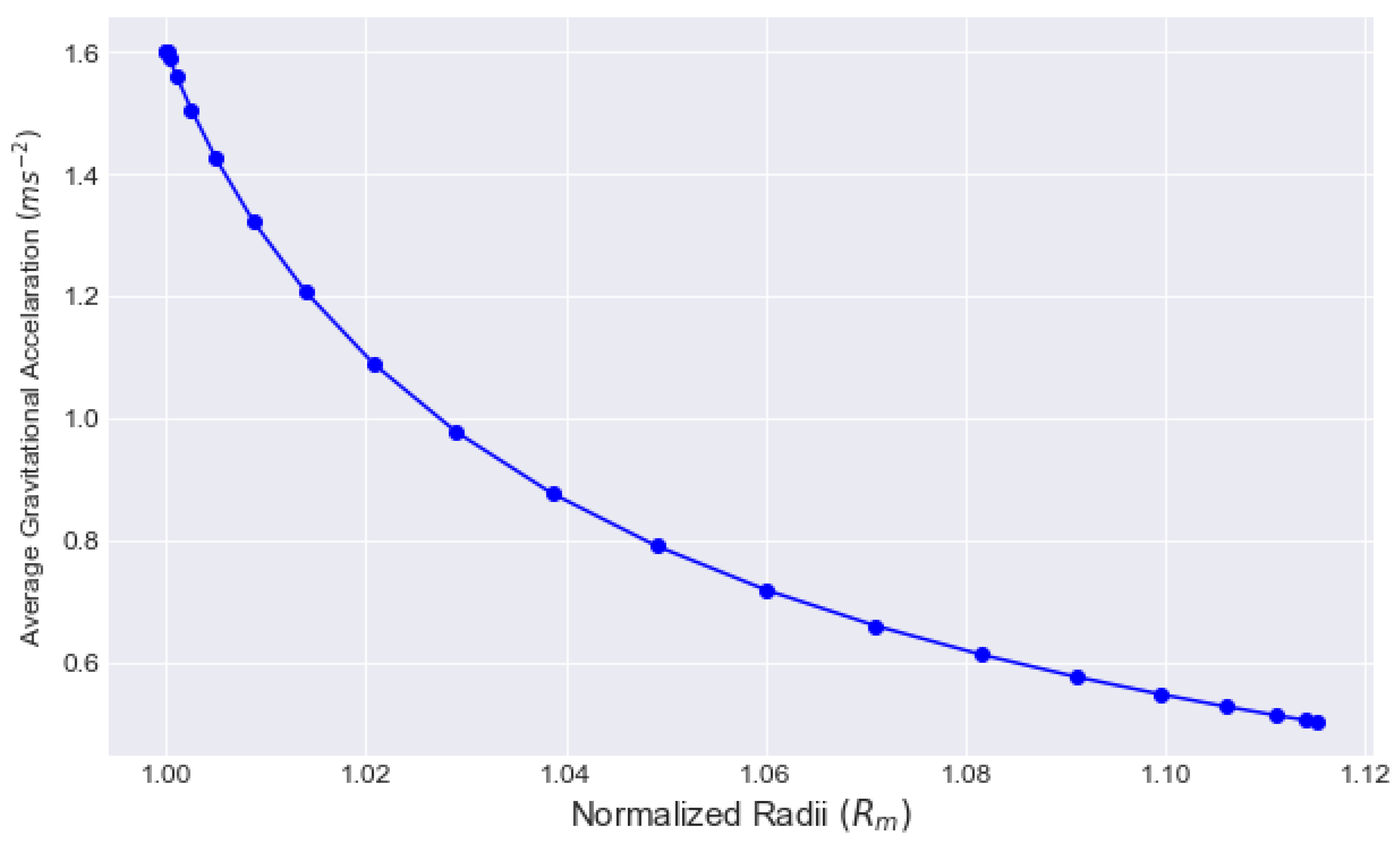
Figure 11 qualitatively displays a prompt decay of gravity anomalies in a finite element where the contours created by the gravitational acceleration perturbation at three radii located at the surface, 100 km, and 200 km above the surface. These coefficients can then be used to approximate orbital propagation at different radii on or above the lunar surface. When considering the coefficients to be a function of radius, we can use the two-dimensional approximations on each surface to promote three dimensions by representing each coefficient as an orthogonal Chebyshev function of radius. As a result, an average surface gravity acceleration value of
was found for a polynomial order of 18 and at 200 km above the surface of the Moon, an average value of
. These results are illustrated in
Figure 12 for all computed radii.
4. FEM Application in Astrodynamics: Satellite Trajectory Propagation
In this section, we will discuss how the FEM can be applied to orbit trajectory propagation, and then we will examine a case study to demonstrate how the coefficients produced from our FEM lunar model can aid in satellite trajectory propagation. Finally, we will compare this result to an SH routine to analyze computational time and precision.
Modeling spacecraft trajectories has been one of the most important fields in astrodynamics and space guidance. Satellite orbit propagation predicts how an object will move based on its current state. The satellite’s position is defined by a group of approximate equations of motion where the degree of approximation is dependent on orbital information. A trajectory is the path a spacecraft follows through space as it is influenced by the gravitational force of one or more bodies, creating acceleration. The two-body model describes of a satellite with negligible mass orbiting a larger astronomical body. The equations of motion for this model can be solved, resulting in different conic sections depending on their distance away from the larger body. Although not represented in the two-body model, it is worth noting that when considering a satellite orbiting the Moon, we would need to consider the gravity of Earth. Introducing an “n-th” body example is to be investigated in future works.
In the equation of motion, the larger astronomical body is treated as fixed within the two-body frame. We then consider the body as a uniform point mass to further simplify the equation of motion. As stated previously, the spacecraft has negligible mass compared to the main body, which means its acceleration is only due to the gravity of the main body.
The following equation represents the two-body problem we implemented using our FEM coefficients (represented by the disturbance acceleration):
where
is the gravitational constant of the Moon provided by the original ‘LP100K’ model:
alongside the disturbance acceleration where
is the
coefficient of
k gravity spherical harmonic perturbation terms. These terms were previously saved from the original FEM model.
As mentioned previously, we can approximate the position of a spacecraft at any point in its orbit as long as we have at least one reference point to use as a starting approximation. Numerical methods of orbit propagation, also termed special perturbations, compute and approximate solutions of general equations of motion [
47,
48,
49].
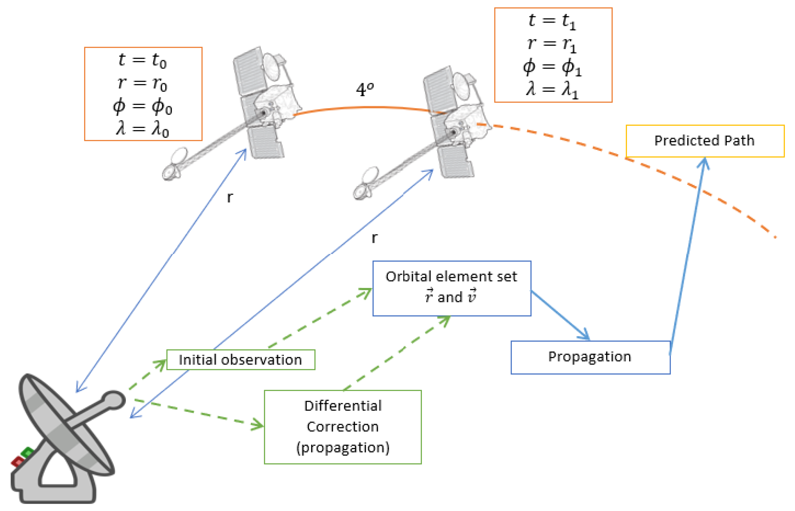
Figure 14 illustrates a general approach to satellite trajectory propagation provided initial conditions. In the following sections, we seek to implement the coefficients acquired from the FEM routine done on a small patch of
square degrees on various radii on and from the surface of the Moon to interpolate the trajectory of a point source satellite orbiting the Moon. Finally, we check the accuracy and computational time to that of the original LP (100 x 100) SH model. Orbital propagation using FEM has been implemented in a series of projects, some of which can be seen here: [
50,
51,
52].
4.1. Trajectory Propagation Using FEM versus LP (100 x 100) SH Gravity Model
In this section, we compare the trajectory propagation results achieved using the coefficient values found from our FEM model to the classical SH method. Computations for the following examples were performed using a machine with the following configurations:
Intel(R) Xeon(R) CPU 3.70GHz 3.70 GHz, 16.0GB of RAM
Windows 64-bit operating system, x64-based processor
MATLAB R2019a
Our final goal in this experiment is to justify that the coefficients produced by the original FEM routine can be used in various satellite orbit propagation problems. The steps needed to take for our orbit propagation experiment are the following:
Produce a set of initial values: , , and R. These values represent the spacecraft’s azimuth, elevation, and radius from the lunar surface, respectively, at .
Set an “ending” position or time. This can be done by providing , or providing a time span.
Produce a small trajectory across a small shell. Using the coefficient values saved at a particular radius from our previous FEM routine to calculate the acceleration of the spacecraft along this initial trajectory using both the FEM and SH approaches. At this point, we will then compare the resulting computational time and error between the two methods.
Generate satellite positions. Using MATLAB’s “ode45” function to solve the differential two-body problem represented as Equation 4.4, we feed in the acceleration values calculated from step 3, and a time span to find the spacecraft’s position as a function of time.
Generate satellite velocities. To do this, we will implement the MATLAB function “fsolve” to solve the systems of nonlinear equations of several values to solve for the satellite’s velocity over the course of the small shell provided initial velocities of , , , the spacecraft’s position, and the time span.
Generate a long-span satellite orbit trajectory. This will be done by, again, utilizing the “ode45" function to generate satellite positions at a longer time span and the resulting final velocities.
Before determining the entire trajectory of a spacecraft, we first have to simulate a smaller portion of its trajectory based on three different radii above the lunar surface (100 km, 150 km, and 200 km). This small trajectory will span over the (4 x 4) square degrees shell at this radius. In this analysis, we consider three tests on orbit propagation. These tests differ in how we produce the initial values:
-
Test 1: Randomized position changes. Using MATLAB’s “rand" function, we randomize a uniformly distributed pseudorandom set of values for
and
, i.e. the changes in azimuth and elevation, respectively. Using these randomized values, we create two ranges for
and
:
With these simulated ranges and a radius 100 km above the lunar surface, we can then convert these values into Cartesian coordinates to get our starting x, y, and z positions of the simulated spacecraft..
Test 2: A Monte Carlo simulation of initial conditions. With this approach, we repeated randomized values for and under the conditions that and . This produces various amounts of ranges for and in which we seek to use a randomly picked set of ranges to achieve the initial positions of the simulated spacecraft.
Test 3: Set starting and final positions. This approach is the most simple and straightforward as it is reflective of the most basic problems in orbit propagation. We start of with converting , , and R into the satellite’s initial Cartesian coordinate: , , and . Unlike the previous two approaches, in this test, the satellite’s final position is found by converting , , and R into the satellite’s final Cartesian coordinate: , , and . All that is left to do is to find the satellite’s positions during and .
For all three approaches, we use the initial ranges of
and
and
R to generate satellite accelerations using our FEM routine and the LP
SH routine. In the FEM analysis, the coefficients saved from our original model at
were multiplied by the Chebyshev polynomials approximated at each elevation and azimuth. These results are then compared to SH results for computational time and error.
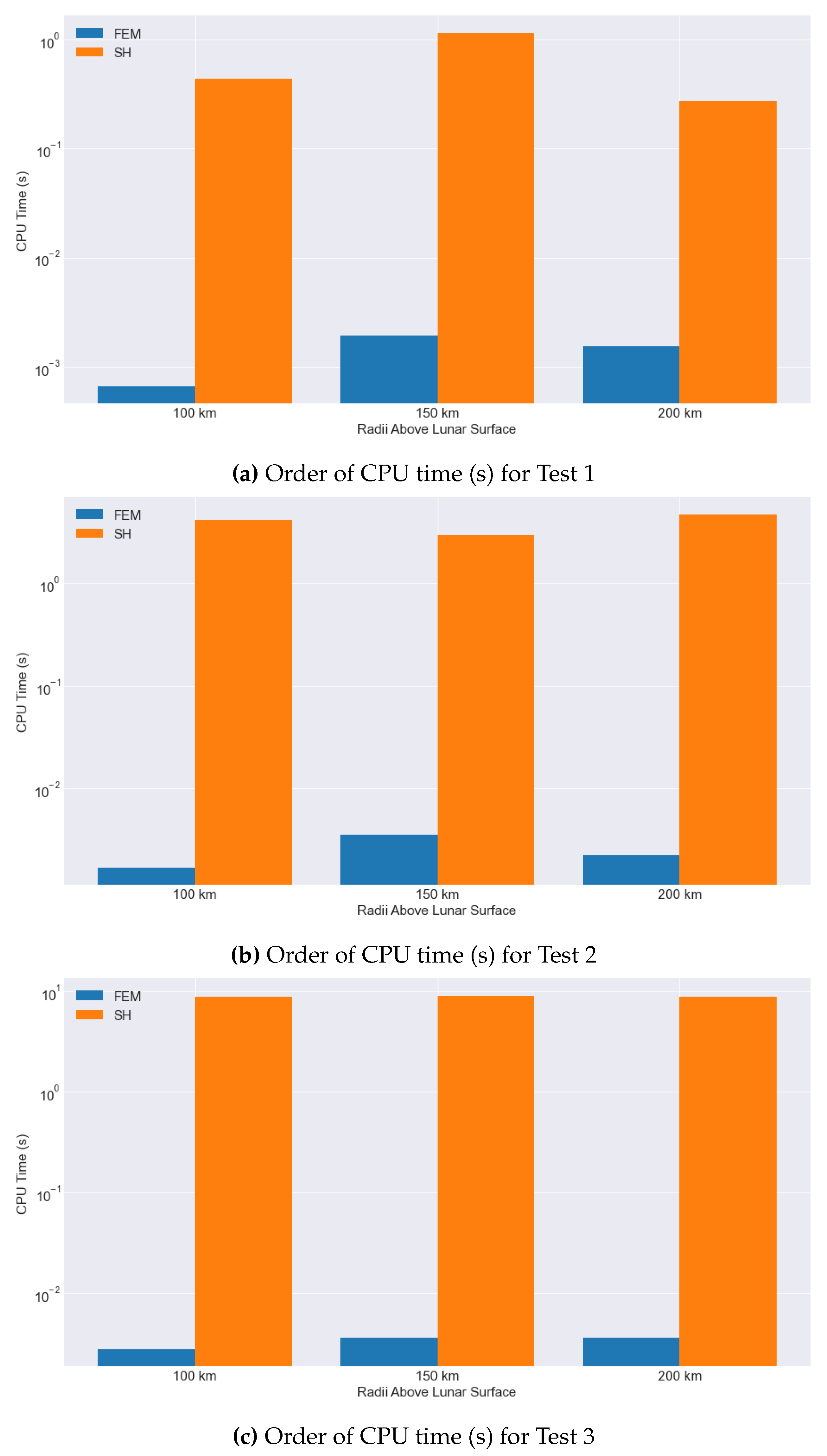
Figure 15 displays the computational time for both approaches for each of the three tests for each of the three radii. For all three tests, FEM timing is 3–4 orders of magnitude smaller than that of SH.
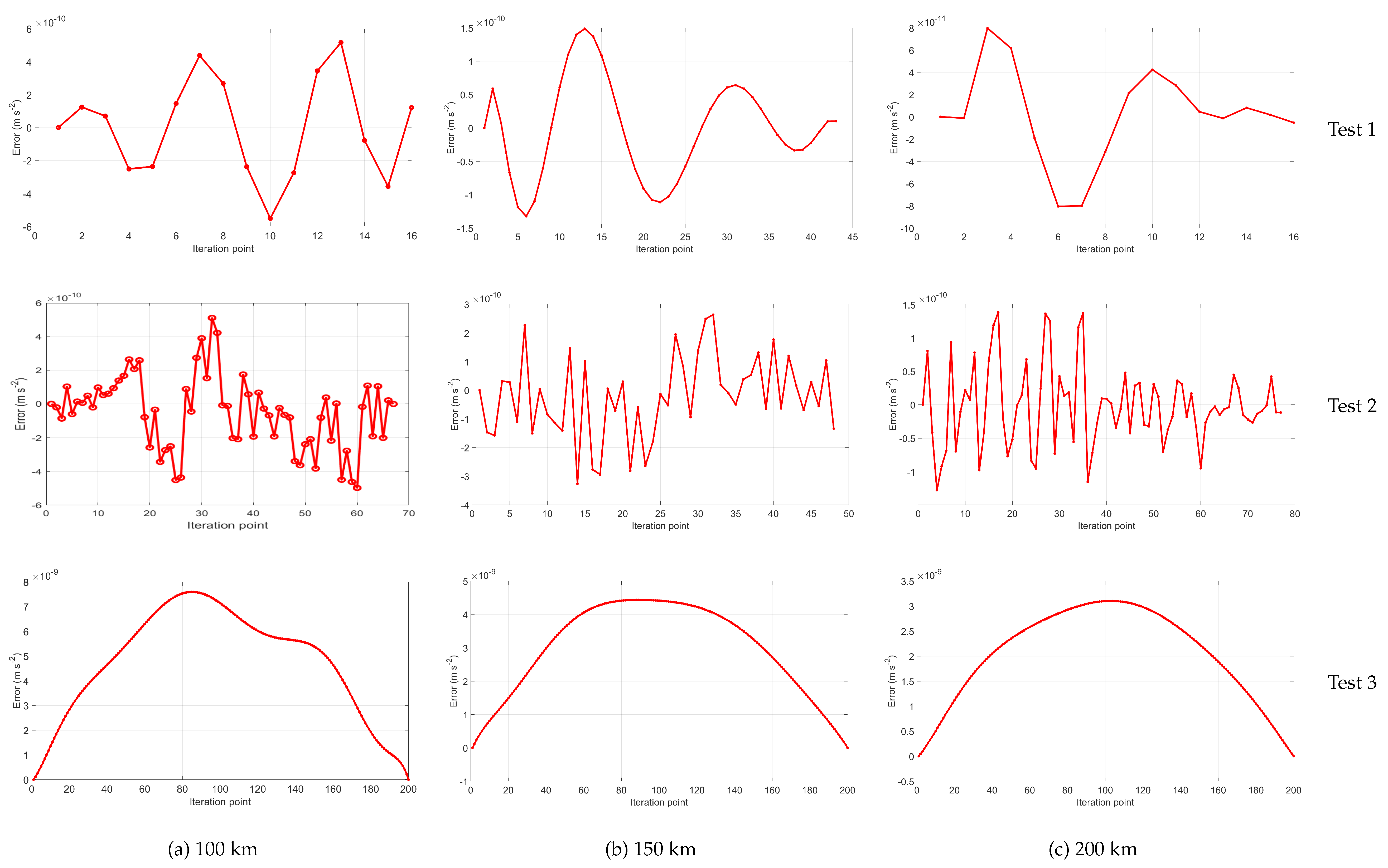
For all three tests, we calculate the FEM model’s error by subtracting it from the “truth” value which we have specified before to be the LP
model. The resulting errors are illustrated in
Figure 16. In Tests 1 and 2, the resulting FEM error from all three radii is in the order of
. With the previously mentioned increase in computational speedup, we find that these two approaches produced above-adequate results for approximating the acceleration beginning produced in the
square degree shell 100 km above the lunar surface. However, for the Monte Carlo simulation (Test 2), we find a higher order of points in the iteration compared to Test 1, which is reflected in the computational time required for each of the tests.
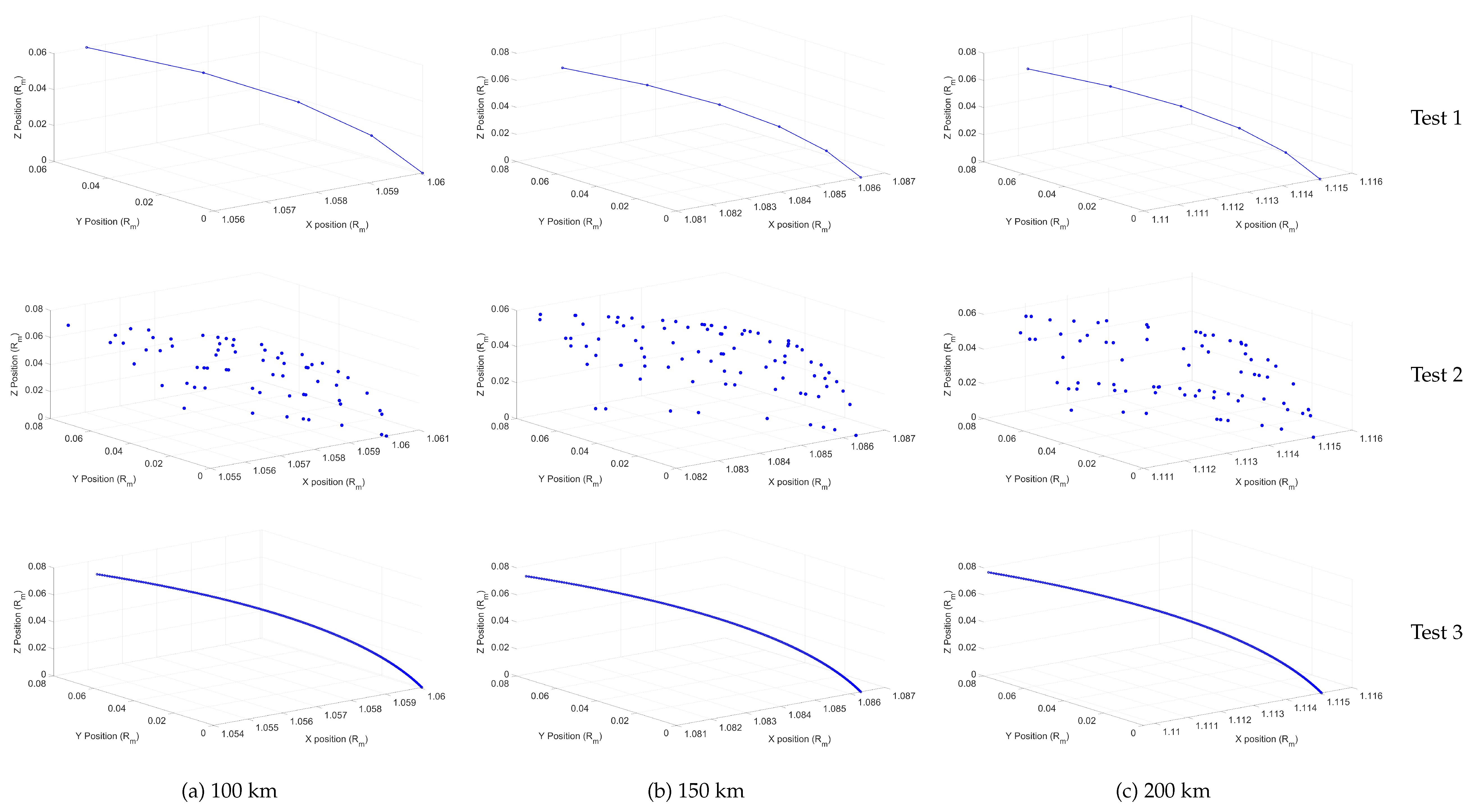
Figure 17 displays the initial trajectories created from these three tests over the
square degree section. In Test 1, the trajectory is smooth and laminar, which is expected from a small spacecraft trajectory, while Test 2 displays a randomized path which is representative of a typical Monte Carlo simulation. It is good to note that the trajectory found in Test 2 does not suggest that the model failed to produce a correct spacecraft orbit. This proves that the model was able to approximate a disorderly trajectory, as apparent in the small error.
The error found in Test 3 is in the order of
across all three radii. It is also good to note that the error is lowest at the “end” points of the calculation due to the initial values set at each starting position. As illustrated in
Figure 17c, the trajectory across the
square degree shell is similar to that of the trajectory for Test 1; however, this Test produced more data points.
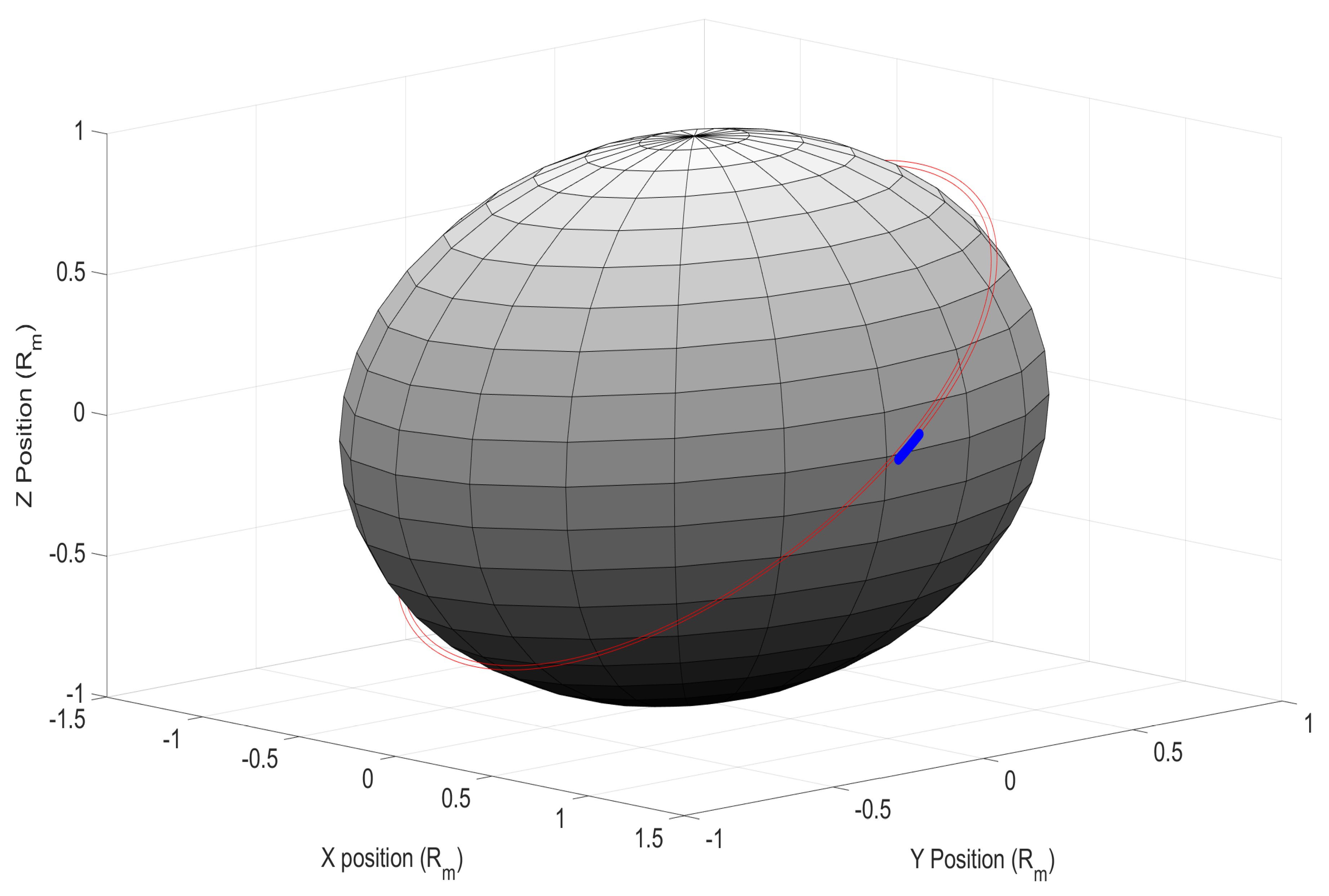
Finally, a long space orbit propagation was done for all three tests. For this, a time span of 360 minutes was used.
Figure 18 shows the long-span predicted trajectory of the satellite as apparent from Test 3 for a radius of 100 km above the lunar surface as an example. This long-span trajectory is shown in red, while the initial small shell trajectory is in blue. The shape of this conic section is representative of typical trajectories found with two-body applications: [
53,
54,
55].
This application of FEM shows promising results and demonstrates a potential path to significant advancements in computational speedup and precision for differential equations in astrodynamics.
5. Conclusion
This research presented a novel approach for modeling the Moon’s surface gravity anomaly, enhancing approximation techniques for Laplace’s differential equations of gravitational forces. Using the orthogonal Finite Element Method (FEM), we approximated a gravitational acceleration model based on data from NASA’s Lunar Prospector mission encompassing 100 spherical harmonic degrees. The FEM model was then compared to the classical SH solution in two regards: accuracy and computational expense.
Our findings revealed the efficiency of orthogonal approximation techniques, including modifying the regression matrix, to be Kronecker factorable when approximating higher dimensions using algebraic identities on the one-dimension orthogonal least-squares operators. The use of Chebyshev polynomials in our approximation strategy has also allowed the selection of specific orthogonal basis functions, which supports an efficient sampling mechanism.
We further evaluated two radial sampling techniques and established that cosine sampling alleviated the challenges associated with the Runge Phenomenon. Placing a conservative error tolerance of on the resulting disturbance acceleration, we were able to save the corresponding coefficient values for reaching radial iteration from the lunar surface to 200 km above. Through our FEM technique, we found a correlation between the number of coefficients resolved in each radial iteration and the polynomial order. For instance, with a polynomial order N=18N=18, we deduced 361 orthogonal polynomial terms on the lunar surface. As a result, an average surface gravity acceleration value of was found for a polynomial order of 18 and at 200 km above the surface of the Moon, an average value of .
A notable highlight was the computational speedup achieved using the FEM approach. We showed that a five-order of magnitude speedup in the computational time can be obtained using the FEM model compared to the original SH approach. As a consequence, a push to apply these techniques on precise long-term orbit propagation for spacecraft and satellites in lunar-based missions has been made. Three numerical orbital tests were conducted for a satellite orbiting the Moon. In all three tests, the coefficient values produced from the original FEM model were used to approximate the satellite’s trajectory as it goes across a (4 x 4) square shell 100 km above the surface. These accelerations showed small errors [] across all three tests with a four-order of magnitude speedup in computation time. A long-span trajectory was also achieved using FEM for one of the tests, displaying promising results in the interpolation of orbital mechanics representing the two-body problem.These findings are crucial for precise orbit propagation in various astrodynamics simulations.
Anticipating future endeavors, this research paves the way for advancements in orthogonal approximation theory and orbit propagation. Potential avenues include code parallelization for upgrades in computation efficiency, FEM machine learning benchmarks, implementing n-body orbital propagation for satellites with treated masses, and FEM modeling of the entire lunar surface for more precision in constraining the disturbance gravitational acceleration. With this, FEM surface gravity models can be developed for other spherical and non-spherical astronomical bodies such as Mars, Europa, and comets whose surface gravity anomaly is not well modeled or studied. Overall, this method is well-versed and shows extreme assurance for the realization of new developments in the field of Astronomy and Astrodynamics.
