Demystifying DFT-Based Harmonic Phase Estimation, Transformation, and Synthesis

Preprint

Article

Demystifying DFT-Based Harmonic Phase Estimation, Transformation, and Synthesis

Altmetrics

Downloads

Views

Comments

A peer-reviewed article of this preprint also exists.

This version is not peer-reviewed

Submitted:

30 August 2024

Posted:

03 September 2024

You are already at the latest version

Alerts

Abstract

Many natural signals exhibit a quasi-periodic behavior and are conveniently modeled as a combination of several harmonic sinusoids whose relative frequencies, magnitudes and phases vary with time. The waveform shape of those signals reflects important physical phenomena underlying their generation, which requires that those parameters be accurately estimated and modeled. In the literature, accurate phase estimation and modeling has received much less research effort than frequency estimation, or magnitude estimation. First, this paper addresses accurate DFT-based phase estimation of individual sinusoids in six scenarios involving two DFT-based filter banks and three different windows. It is shown that bias in phase estimation is less than 1E-3 radians when the SNR is equal to or larger than 2.5 dB. Taking as a reference the Cramér-Rao Lower Bound, it is shown that one particular window offers a performance of practical interest by approximating better the CRLB when signal conditions are favorable, and by minimizing the performance deviation when signal conditions are adverse. Second, this paper explains how a shift-invariant phase-related feature can be devised that characterizes harmonic phase structure, which motivates a signal processing paradigm that greatly simplifies parametric modeling, transformation and synthesis of harmonics signals, in addition to facilitating the understanding and reverse engineering of the phasegram. Theory and results are discussed in a reproducible perspective using dedicated experiments that are supported with code allowing not only to replicate figures and results in this paper, but also to expand research.

Keywords:

Subject: Engineering - Electrical and Electronic Engineering

1. Introduction

1.1. Motivation

Many natural and synthetic quasi-periodic signals, including speech, singing, physiological signals such as ECG, music, and acoustic waves reflecting vibrations of mechanical systems, possess a harmonic structure of sinusoids whose magnitudes, phases and underlying fundamental frequency vary with time.

Harmonic phases are very important in defining the waveform shape of quasi-periodic signals and, therefore, are immensely informative regarding the physical phenomena that generate them. Examples include the periodic glottal excitation signal that sheds light on the physiological process governing the vocal fold vibration in the larynx; and periodic acoustic signals that are generated by mechanical systems and that shed light on whether the operation of those systems is correct within a predefined safety margin.

Given that the harmonic phases depend explicitly on the time, they vary much faster than the harmonic magnitudes and fundamental frequency typically do, which has always represented a challenge from the point of view of signal analysis, estimation, interpretation, modeling, transformation and synthesis [1,2,3]. Since accurate frequency and magnitude estimation of sinusoids have been extensively discussed in the literature [4,5,6,7,8,9,10,11], we assume in this paper that these are solved problems and focus, instead, on two problems addressing phase. The first problem concerns practical and accurate DFT-based phase estimation of individual sinusoids. This is instrumental in solving a second problem: parametric modeling of the phase of sinusoids in a harmonic structure and in such a way that is time-shift invariant, interpretable, insightful, and simplifies harmonic signal processing. To our best knowledge, this is the first time such a combined perspective is presented in a manner that is easily apprehensible.

This paper demonstrates that these problems can be tackled in a practical way, which is facilitated by Matlab code that replicates the main results and illustrations presented.

1.2. Problem Statement

This paper is concerned with practical ways of representing quasi-periodic signals using the concepts of structure and parametric modeling. By structure we mean an identifiable form, or organization, and by parametric modeling we mean a simple mathematical formulation that captures that organization and is able to model it using a small number of controllable parameters. We also admit in this paper that signals are quasi-periodic and are locally stationary. Quasi-periodicity means that the waveform shape in a periodic signal varies slowly among at least three adjacent periods, even if their period may increase or decrease. Local stationarity means that harmonic parameters, such as sinusoidal magnitude and frequency, vary slowly with time, such that they can be considered to be approximately constant within a short windowed region of the observed signal.

In order to motivate the main aspect that is discussed in this paper, which is phase representation, estimation and parametric modeling, we address first the concept of structure on the three aspects that define a stationary periodic signal: i) frequency, ii) magnitude, and iii) phase.

Let us consider a real-valued signal

x (t)

that consists of L sinusoids

x (t) = \sum_{ℓ = 0}^{L - 1} A_{ℓ} sin (Ω_{ℓ} t + ϕ_{ℓ}) + s (t),

(1)

where

A_{ℓ}

and

Ω_{ℓ}

represent, respectively, the magnitude and frequency of the

ℓ^{t h}

sinusoid,

ϕ_{ℓ}

represents the starting phase of the

ℓ^{t h}

sinusoid, and

s (t)

represents a random signal without any relevant phase structure. It is well known from basic Fourier theory that the sinusoids in a periodic signal are harmonically related [12]. Hence, in our context,

Ω_{ℓ} = (ℓ + 1) Ω_{0},

(2)

i.e., the frequency of each sinusoid is a multiple integer of a fundamental frequency that is represented by

Ω_{0}

. Thus, this frequency organization represents a frequency-related feature that is intrinsic and, therefore, structural, to any periodic signal. This means that the only information in the frequency structure that is truly unique is the fundamental frequency.

A second structural aspect that defines a periodic signal consists in the organization of the magnitudes of the different harmonics, and can be given by the ratio between the magnitude of each harmonic (

A_{ℓ}

) and that of the fundamental frequency magnitude (

A_{0}

). If the latter is looked at as a gain, then, a given periodic signal is characterized by a normalized magnitude-related feature vector, where the first value is one, and all other values (

A_{ℓ} / A_{0}

) help defining the waveform shape of the periodic signal. This magnitude-related feature vector expresses the magnitude structure of a periodic signal, independently of time, and of the fundamental frequency of the signal, provided that the waveform shape is locally preserved.

A third aspect that contributes to define a particular waveform shape of a periodic signal involves the relationships between the starting phases of the different harmonics,

ϕ_{ℓ}

. Ideally, it would be interesting to characterize the waveform shape of a given periodic signal on the basis of a normalized phase-related feature vector that, similarly to the magnitude-related feature vector, is independent of time and of the fundamental frequency. This paper aims to show that such a time-shift invariant phase-related feature exists, and that it can be extracted using fairly conventional spectrum analysis. Moreover, it can be modeled in simple and insightful ways.

To this end, two problems need to be addressed. The first one, involves estimating the harmonic starting phase values,

ϕ_{ℓ}

, from a short segment of

x (t)

that is representative of the periodic signal. By representative we mean that the short segment contains a few periods having a similar waveform shape but its duration is not related to the period of the periodic signal. The second one, involves establishing a model that is based on the estimated harmonic starting phases, and that when it is combined with harmonic magnitude information, helps to completely explain a given waveform shape in a way that is time-shift invariant, and independent of

Ω_{0}

. The next section discusses further these challenges in a practical perspective and motivates a paradigm in harmonic signal processing that is oriented to harmonic magnitude and phase structure, which eases immensely signal modeling, transformation, and synthesis.

1.3. A Practical Approach to Harmonic Signal Processing

The problem that we address fits in the realm of spectrum estimation using Fourier analysis. Given that we aim at practical signal processing such that it is amenable to real-time operation on low-cost platforms, we highlight simple technical approaches that use the Discrete Fourier Transform (DFT), which allows benefitting from efficient realization algorithms (e.g., the FFT [13]). In addition, we also exclude non-causal or iterative processing in order to accommodate real-time operation on low-cost platforms.

Thus, in a practical setting, simple spectrum estimation implies typically three operations: 1) sampling, 2) Time-Frequency (T-F) transformation, and 3) frequency, magnitude and phase estimation.

A discrete-time version of the signal represented by Equation (1) is first obtained using a convenient sampling frequency ( $F_{S}$ ), i.e.,

$x [n] = {x (t)|}_{t = n T_{S} = \frac{n}{F_{S}}},$

(3)

where $T_{S}$ represents sampling period and corresponds to the reciprocal of the sampling frequency ( $F_{S}$ ).
A T-F transformation (using e.g., the DFT) is computed on a windowed region of the discrete-time signal containing N samples. We assume that N is a power of 2 number. If the window is represented by $w [n]$ (and that we assume is symmetric), this means that, in the case of the DFT, we compute

$X [k] = \sum_{n = 0}^{N - 1} x [n] w [n] e^{- j \frac{2 π}{N} k n}, k = 0, 1, \dots, N - 1 .$

(4)
Finally, a suitable estimation procedure is used that takes as input the spectral coefficients, $X [k]$ , and delivers robust estimates of all the harmonic frequencies, magnitudes, and phases.

These simple spectrum estimation steps enable the identification of important harmonic parameters such as the normalized fundamental frequency,

ω_{0} = Ω_{0} T_{S}

. On the other hand, the parametric representation of the harmonic magnitudes and phases, if done in such a way that it does not depend on the time, nor on the fundamental frequency, paves the way to a harmonic signal processing paradigm that promotes algorithm simplification, flexibility, and even insight.

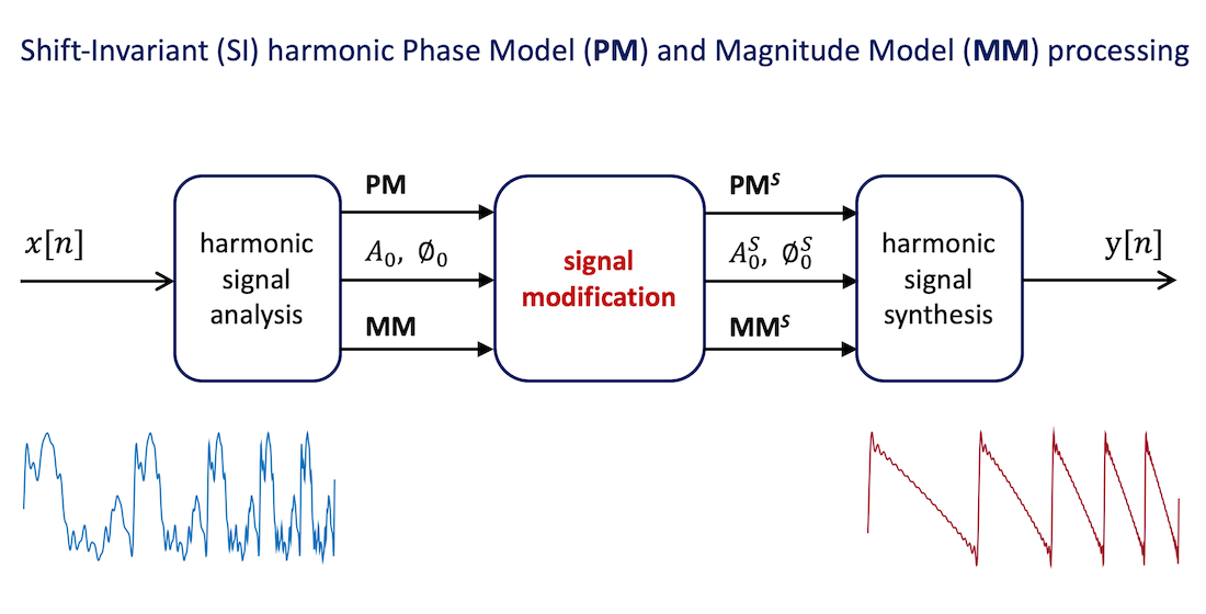
In fact, in many applications involving, for example, speech enhancement, time-scale or pitch scale modification of speech [3], and special effects in singing and music [2], harmonic sinusoids are individually modified in their frequency, magnitude and phase trajectories as Figure 1 suggests.

However, this approach requires careful unwrapping of the phases of all harmonics such that their modification is correct and does not suffer from the errors that may result from the wrapped phase representation in the interval

[- π, π [

. In addition, phase unwrapping, which is carried out for all harmonics on an individual basis and on a `horizontal’ manner, i.e., along the time axis, is itself prone to estimation errors. The most critical aspect of this approach, however, is that it is not insightful, i.e., it does not capture the overall, or holistic, harmonic phase structure, which means that, most likely, it does not explicitly control it. The consequence is that although phase coherence may be obtained on an individual sinusoidal basis, `vertical’ coherence may not be controlled and artifacts may result, the most common being known as `phasiness’ [14].

A more convenient paradigm in harmonic signal processing is represented by the block diagram that is illustrated in Figure 2.

According to this paradigm, harmonic magnitude and phase models are extracted that represent the holistic harmonic structure (or `vertical’ structure) in a way that is time-shift invariant, and independent of the fundamental frequency. This not only promotes insight in terms of the harmonic signal structure, but also facilitates tremendously signal transformation. For example, the magnitude model (MM) and the phase model (PM) may change arbitrarily, or may be interpolated in simple ways. Or, if the waveform shape is to be preserved, they may be left unchanged, and the changes in the synthesis affect only the fundamental frequency parameters (

ω_{0}^{S}

A_{0}^{S}

ϕ_{0}^{S}

). In addition, the synthetic phase

ϕ_{0}^{S}

may be decoupled from the original phase

ϕ_{0}

since it can be easily synthesized using the value of

ω_{0}^{S}

1.4. Paper Structure

This paper is divided into two major parts. The first part, corresponding to Section 2, is devoted to the estimation of the phases of individual sinusoids using light but robust DFT-based analysis procedures. Two commonly used DFT filter banks and three window functions are considered. Robust phase estimators are found taking into consideration the specificities of the filter banks, and of the window functions, notably their frequency responses. It is shown that the relative performance of the six phase estimation alternatives depends mainly on the main lobe width of the magnitude of those frequency responses, and the associated near-end and far-end leakage properties. In particular, taking the Cramér-Rao Lower Bound (CRLB) as a reference, it is shown that the performance of one of the studied windows is not only closer to the CRLB, but also offers a lower deviation when signal conditions are more adverse.

In the second part of the paper, corresponding to Section 3, we address the computation of a time-shift invariant harmonic phase model (HPM) that implements the holistic PM that is represented in Figure 2 and that validates the harmonic signal processing paradigm that the block diagram of Figure 2 substantiates. Using the concepts of vertical phase coherence, as well as detailed and interpretable test cases, both ground-truth and estimated PM are illustrated and compared under various test conditions. This section concludes with the illustration of HPM of actual natural voice signals, and the explanation of its usefulness in demystifying the phasegram of a representative periodic signal. Finally, Section 4 concludes this paper with a summary of the most significant concepts and results presented, in addition to a perspective on further research and application scenarios.

2. Robust DFT-Based Phase Estimation of Individual Sinusoids

Our purpose in this section is to estimate the starting phases (

ϕ_{ℓ}

) of all sinusoids in a harmonic signal, as in (1), after the signal has been subject to simple uniform sampling as in (3), multiplied by a window (

w [n]

), and the result is transformed to a discrete-frequency Fourier domain such as (4). As we admit in Section 1.1, and as it is illustrated in Figure 1 and in Figure 2, we rely on a pre-existing harmonic analysis framework that is able to deliver not only an accurate fundamental frequency estimate (

ω_{0}

), but also harmonic magnitude estimates (

A_{ℓ}

). In our simulations, in this paper, we use ground-truth test signals such that those parameters are known beforehand. This is equivalent to assuming that these parameters are estimated without error.

Given a certain magnitude spectrum describing a harmonic signal, it is very tempting to think that the estimated harmonic starting phases can be taken as the phases of the DFT spectral lines (or DFT bins) corresponding to local maxima in the magnitude spectrum. In other words, if

X [k]

k = 0, 1, \dots, N - 1

, represents the Fourier spectrum of the windowed harmonic signal, and if

k_{ℓ} = \overset{[}{k}] argmax | X [k] |

, with

ℓ = 0, 1, \dots, L - 1

, denotes a DFT bin index representing a local maximum in the magnitude spectrum and corresponding to harmonic ℓ, it is very tempting to believe that

ϕ_{ℓ}

can be estimated as

{\hat{ϕ}}_{ℓ} = ∠ X [k_{ℓ}]

. In fact, this equation is not correct given that estimations must take into consideration the specificity of the time-frequency transformation, the specificity of the window, and the relation between each spectral peak in the magnitude spectrum and the fundamental frequency.

As an important contribution of this paper, this section highlights that phase estimation does not depend on accurate frequency estimation of individual sinusoids. In fact, as stated by Rife and Boorstyn, most practical DFT-based accurate frequency estimators involve a two-step approach: a coarse search that is followed by a fine search [10]. The first step is almost trivial as it involves only peak picking and the second is what determines the accuracy of the frequency estimator [4]. Usually, sinusoidal magnitude estimation depends on the result of the fine search step in frequency estimation and, as consequence, the accuracy of the former depends on the accuracy of the latter. In this section, we show that accurate phase estimation does not depend on this fine search step in frequency estimation and, therefore, its accuracy depends mainly on the severity of the SNR.

In order to illustrate different possibilities, we consider six cases that result from the combination of two different DFT-based filter banks, and three different windows.

In order to simplify results and in order to facilitate their comparison, in all six cases we consider the analysis of just one harmonic sinusoid in (1), i.e. we consider that after sampling according to (3), our signal is

x [n] = A_{ℓ} sin (ω_{ℓ} n + ϕ_{ℓ}) + s [n] .

(5)

In this equation,

ω_{ℓ} = Ω_{ℓ} T_{S} = \frac{2 π}{N} (k_{ℓ} + Δ_{ℓ}),

(6)

where

k_{ℓ}

represents the bin index (or sub-band channel) corresponding to a local maximum in the magnitude spectrum, and

Δ_{ℓ}

represents fractional frequency. Depending on the type of the T-F transformation, and depending on the window that is used, the continuous interval of

Δ_{ℓ}

may be either

[- 0.5, 0.5 [

[0.0, 1.0 [

. The rationale for this will be explained next.

2.1. DFT and the Rectangular window

In this subsection, the frequency-domain representation of our sinal (5) is obtained by computing the DFT according to (4) when the window is the Rectangular window:

w [n] = w_{R} [n] = 1, n = 0, 1, \dots, N - 1 .

(7)

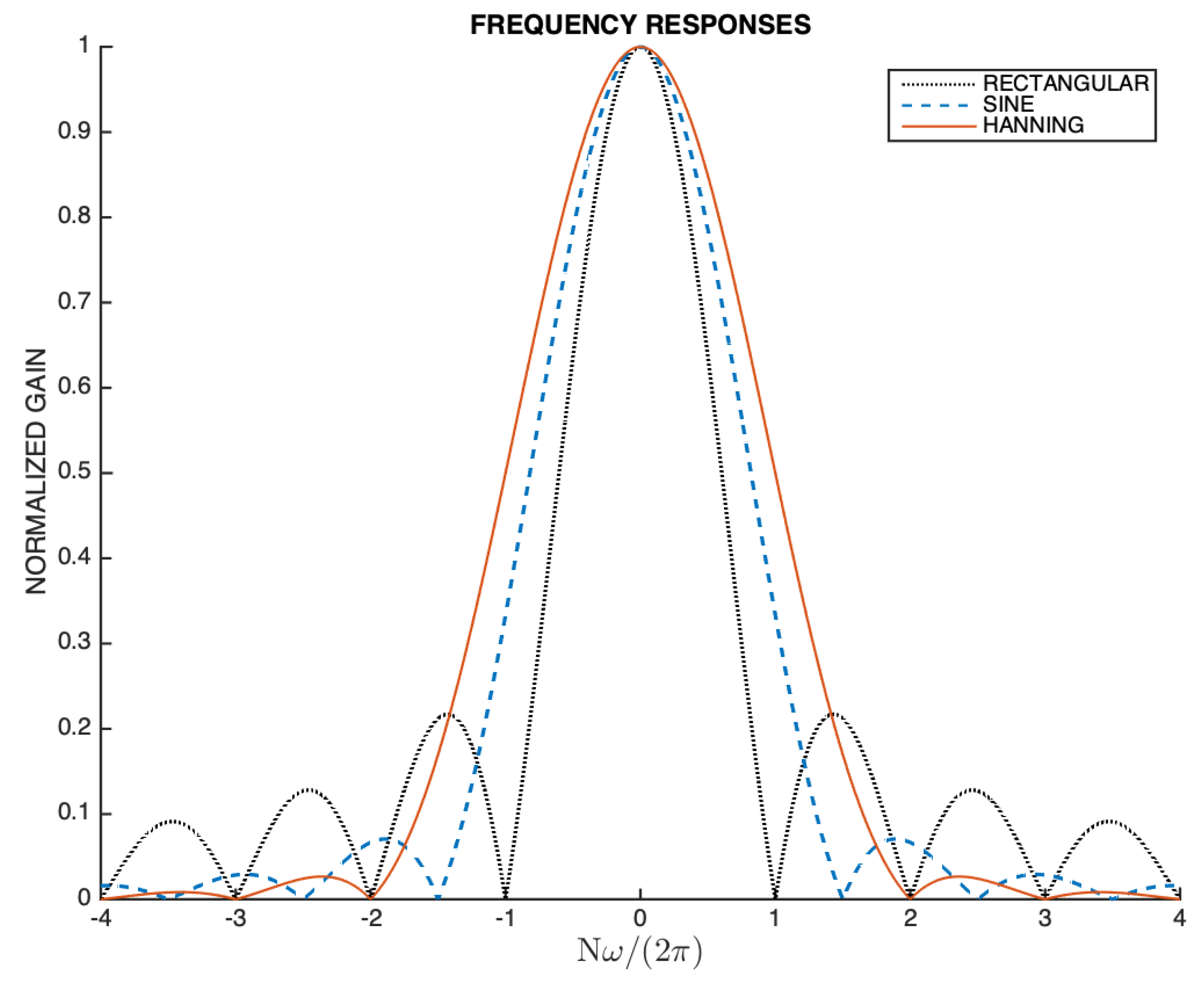
Figure 3 represents the magnitude of the frequency response of the Rectangular window, i.e.,

|W_{R} (e^{j ω})| = |\sum_{n = 0}^{N - 1} w_{R} [n] e^{- j ω n}|

, in the range

- 8 π / N \leq ω \leq 8 π / N

, and after a gain normalization such that the maximum gain is the unity. Two other frequency responses are also represented in Figure 3 that will be discussed in subsequent subsections. The frequency axis in Figure 3 is normalized by

2 π / N

such that integer numbers in this normalized axis can be read as bin index in a DFT filter bank interpretation.

Given that both

x [n]

and

w [n]

in (4) are real-valued, then

X [k]

is known to be conjugate-symmetric, i.e.,

X [k] = X^{*} [N - k]

k = 1, 2, \dots, N / 2 - 1

, where

{(\cdot)}^{*}

denotes complex-conjugation. This means that the information provided by

X [k]

that is unique lies in the range

k = 0, 1, \dots, N / 2

. Using Euler trigonometric relations and ignoring the Dirichlet kernel (i.e., a function having the form

sin (θ) / sin (θ / N)

) that is centered outside this range of k and that causes spectral leakage, we are left with

X [k] \approx \frac{A}{2} e^{j (ϕ_{ℓ} - \frac{π}{2} + π (k_{ℓ} + Δ_{ℓ} - k) (1 - \frac{1}{N}))} \frac{sin π (k_{ℓ} + Δ_{ℓ} - k)}{sin \frac{π}{N} (k_{ℓ} + Δ_{ℓ} - k)} .

(8)

Given that the width of the main lobe of the frequency response of the Rectangular window is

4 π / N

, as it is apparent in Figure 3, then, depending on the value of

Δ_{ℓ}

, at most two spectral lines having a non-zero magnitude fall within that main lobe width. If

Δ_{ℓ} \in [- 0.5, 0.5 [

, then the spectral line

k = k_{ℓ}

corresponds to a local maximum in the magnitude spectrum, as it is illustrated in Figure 4.

This means that this spectral line is more likely to be less affected by noise and leakage, which makes it particularly suitable for phase estimation. In fact, if

k = k_{ℓ}

, then from (8) we obtain

∠ X [k_{ℓ}] = ϕ_{ℓ} - \frac{π}{2} + π Δ_{ℓ} (1 - \frac{1}{N})

, which leads to

ϕ_{ℓ} = ∠ X [k_{ℓ}] + \frac{π}{2} - π Δ_{ℓ} (1 - \frac{1}{N}) .

(9)

Despite being usable, this result presents one practical difficulty since it requires that the fractional frequency be first estimated as accurately as possible [4,15]. This means that frequency estimation errors may propagate to the phase estimation. In order to avoid this, a more robust approach is available if, instead of estimating phase with respect to the origin of the time segment, estimation is performed with respect to the group delay of the DFT filter bank. Given that the window is symmetric, the group delay is constant and is given by

τ = (N - 1) / 2

. Therefore, using this result and using (6) and (9), we obtain

\begin{matrix} {\hat{ϕ}}_{ℓ} & = & ∠ X [k_{ℓ}] + \frac{π}{2} - π Δ_{ℓ} (1 - \frac{1}{N}) + ω_{ℓ} τ \\ = & ∠ X [k_{ℓ}] + \frac{π}{2} + π k_{ℓ} (1 - \frac{1}{N}), \end{matrix}

(10)

which represents a more robust phase estimator that just depends on the bin index of the spectral line corresponding to the local maximum, and on the phase of that spectral line.

A perspective on the estimation error that is associated with (10) can be given by a simple metric that evaluates the cumulative distance, or error, between the estimated

\hat{ϕ}

, and the corresponding ground-truth value,

ϕ

, when the latter varies in the range

[- π, π [

. For illustration purposes, we use the error metric as in (11), we create a ground-truth signal using (5), and configure the noise (

s [n]

) such that the SNR is 30 dB in one case, and 10 dB in another case. In each case, we evaluate the cumulative phase estimation error as a function of the fractional frequency,

Δ_{ℓ}

E R R O R = \int_{- π}^{π} |e^{j ϕ} - e^{j \hat{ϕ}}| d ϕ

(11)

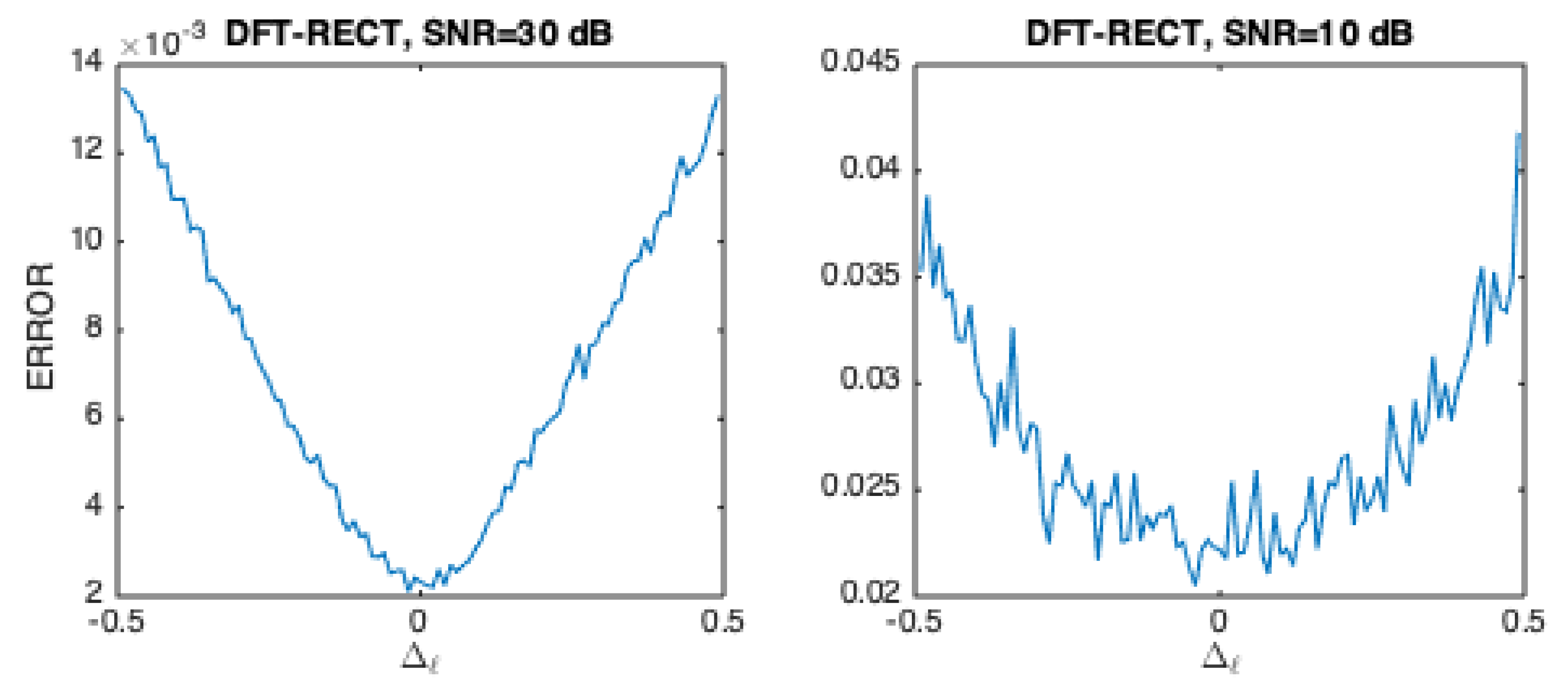
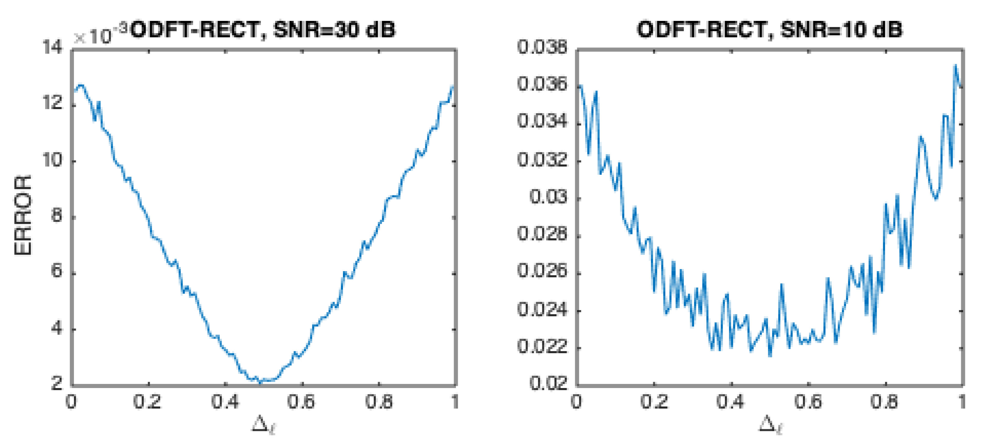
Figure 5 represents the results when

N = 128

and

ℓ = 13

It can be seen that the estimation error distribution is consistent with the relative magnitudes of adjacent spectral bins as illustrated in Figure 4. In fact, when

Δ_{ℓ}

approaches

- 0.5

, or

0.5

, the cumulative error increases relative to the case when

Δ_{ℓ} = 0

, which is a consequence of the fact that the magnitudes of two adjacent spectral lines become comparable and significantly lower than the maximum value they can reach (when

Δ_{ℓ} = 0

), which not only exacerbates leakage effects, but also increases vulnerability to the noise influence. Due to the specific frequency response of the Rectangular window, as Figure 3 and Figure 4 highlight, then, when

Δ_{ℓ} = 0

and the SNR is infinity, the spectral leakage is zero and phase is estimated without error. The Matlab code generating Figure 5 is available (estimatePHASE_DFT_rect.m), which facilitates that other values of N, ℓ, or SNR can be tried.

2.2. DFT and the Sine and shifted Hanning Windows

Other windows offering a better main-to-side lobe attenuation when compared to the Rectangular window are frequently used in spectrum estimation and FIR filter design [13]. Although standard Hamming or Hanning windows could be used in our analysis, we use two convenient windows that happen to be related, and that are especially important in perfect reconstruction filter banks [16,17], such as those that are frequently used in audio coding and general analysis-synthesis [18]. One window is known as the Sine window and is defined as

w_{S} [n] = \sqrt{w_{H} [n]} = sin \frac{π}{N} (n + 0.5), n = 0, \dots, N - 1,

(12)

where

w_{H} [n]

represents the shifted Hanning window that is defined as

w_{H} [n] = \frac{1}{2} [1 - cos \frac{2 π}{N} (n + 0.5)], n = 0, \dots, N - 1 .

(13)

When the Sine window is used in the DFT analysis according to (4), where

x [n]

is a noisy sinusoid given by (5), then, using an approach that is similar to that used in the previous subsection, the spectral line corresponding to the relevant local maximum in the magnitude spectrum (

| X [k_{ℓ}] |

) can be approximated by

X [k_{ℓ}] \approx \frac{A}{4} e^{j (ϕ_{ℓ} - \frac{π}{2} + π Δ_{ℓ} (1 - \frac{1}{N}))} F (Δ_{ℓ}),

(14)

where

F (Δ_{ℓ}) = \frac{sin π (Δ_{ℓ} + \frac{1}{2})}{sin \frac{π}{N} (Δ_{ℓ} + \frac{1}{2})} + \frac{sin π (Δ_{ℓ} - \frac{1}{2})}{sin \frac{π}{N} (Δ_{ℓ} - \frac{1}{2})} .

(15)

In the case of the shifted Hanning window, the local maximum in the magnitude spectrum can be approximated by

X [k_{ℓ}] \approx \frac{A}{4} e^{j (ϕ_{ℓ} - \frac{π}{2} + π Δ_{ℓ} (1 - \frac{1}{N}))} G (Δ_{ℓ}),

(16)

where

G (Δ_{ℓ}) = 2 \frac{sin π Δ_{ℓ}}{sin \frac{π}{N} Δ_{ℓ}} + \frac{sin π (Δ_{ℓ} + 1)}{sin \frac{π}{N} (Δ_{ℓ} + 1)} + \frac{sin π (Δ_{ℓ} - 1)}{sin \frac{π}{N} (Δ_{ℓ} - 1)} .

(17)

It can be easy concluded that the

F (Δ_{ℓ})

and

G (Δ_{ℓ})

functions have the same polarity when

Δ_{ℓ} \in [- 0.5, 0.5 [

and, thus, they do not affect the phase in this particular range of

Δ_{ℓ}

. On the other hand, comparing (14), (16), and (8) when

k = k_{ℓ}

, it can be concluded the phase is governed by the same function, which is a consequence of the fact that all three windows share the same linear-phase property, and the same group delay. This also means that in all three cases the phase can be estimated using Equation (10), although the quality of the phase estimation depends on each window due to its specific near-end and far-end leakage properties.

As it is apparent in Figure 3, the width of the main lobe of the frequency response is

6 π / N

in the case of the Sine window, and

8 π / N

in the case of the shifted Hanning window [4,8]. This implies that, depending on the value of

Δ_{ℓ}

, at most three spectral lines having a non-zero magnitude fall within that main lobe width of the Sine window frequency response. In the case of the shifted Hanning window, the number of spectral lines is four. As in the previous subsection, if

Δ_{ℓ} \in [- 0.5, 0.5 [

, then the spectral line

k = k_{ℓ}

corresponds to a local maximum in the magnitude spectrum when the Sine window or the shifted Hanning window are used. Figure 6 illustrates the case corresponding to the Sine window.

Although this figure resembles Figure 4, two important aspects are worth noting. First, the side lobe attenuation decay (not shown in these figures) is stronger for the Sine window, when compared to the Rectangular window [4]. Second, because the main lobe of the frequency response of the Sine window is wider than the main lobe of the Rectangular window, this means that when

Δ_{ℓ}

is such that the magnitudes of the spectral lines

k = k_{ℓ} - 1

and

k = k_{ℓ}

become comparable, or the magnitudes of the spectral lines

k = k_{ℓ}

and

k = k_{ℓ} + 1

become comparable, these magnitudes are closer to the maximum value they can reach (which takes place for

Δ_{ℓ} = 0.0

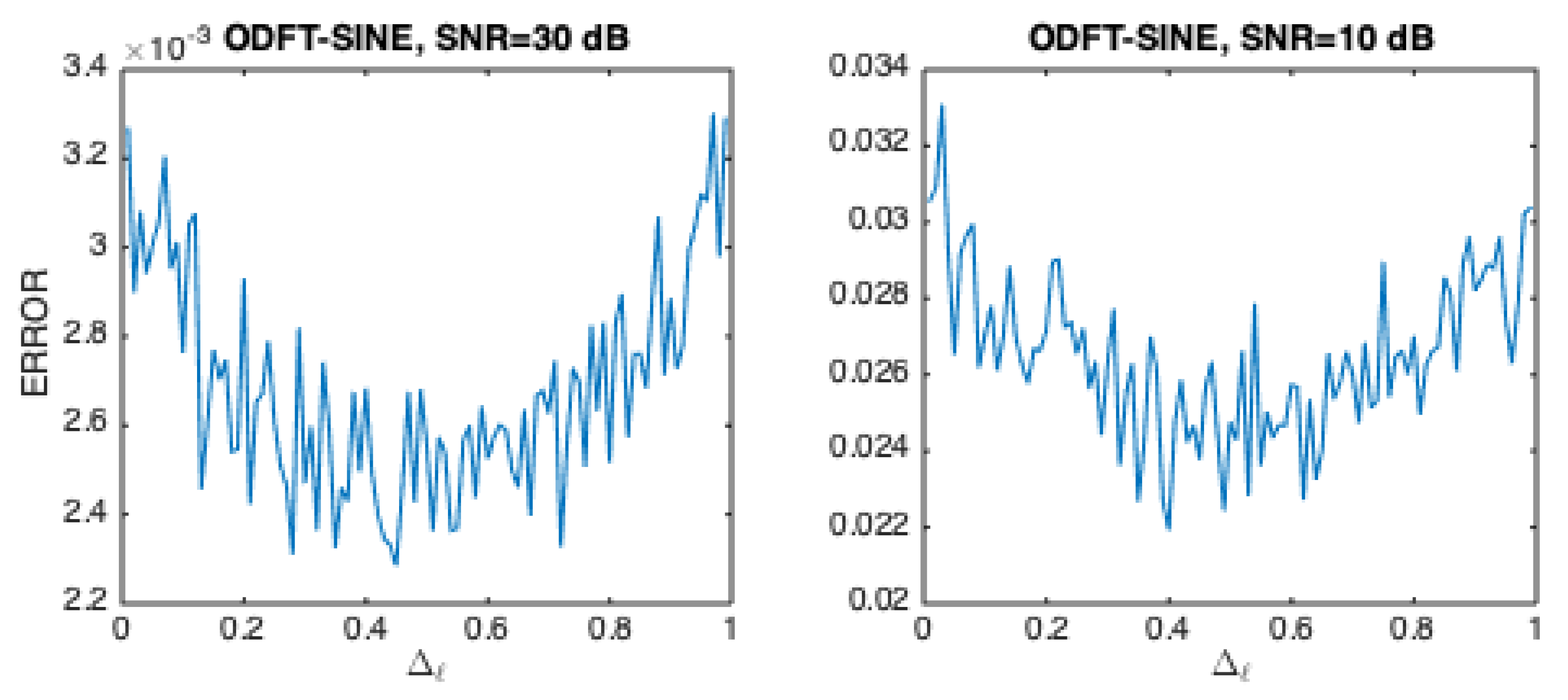
) than what happens for the Rectangular window. These concurrent reasons make that relative to the case of the Rectangular window, phase estimation using the Sine window is likely to be more immune to the noise influence, and to suffer less leakage effects. This can be confirmed by making a simple study on the phase estimation error, as it was described in the previous subsection for the Rectangular window. 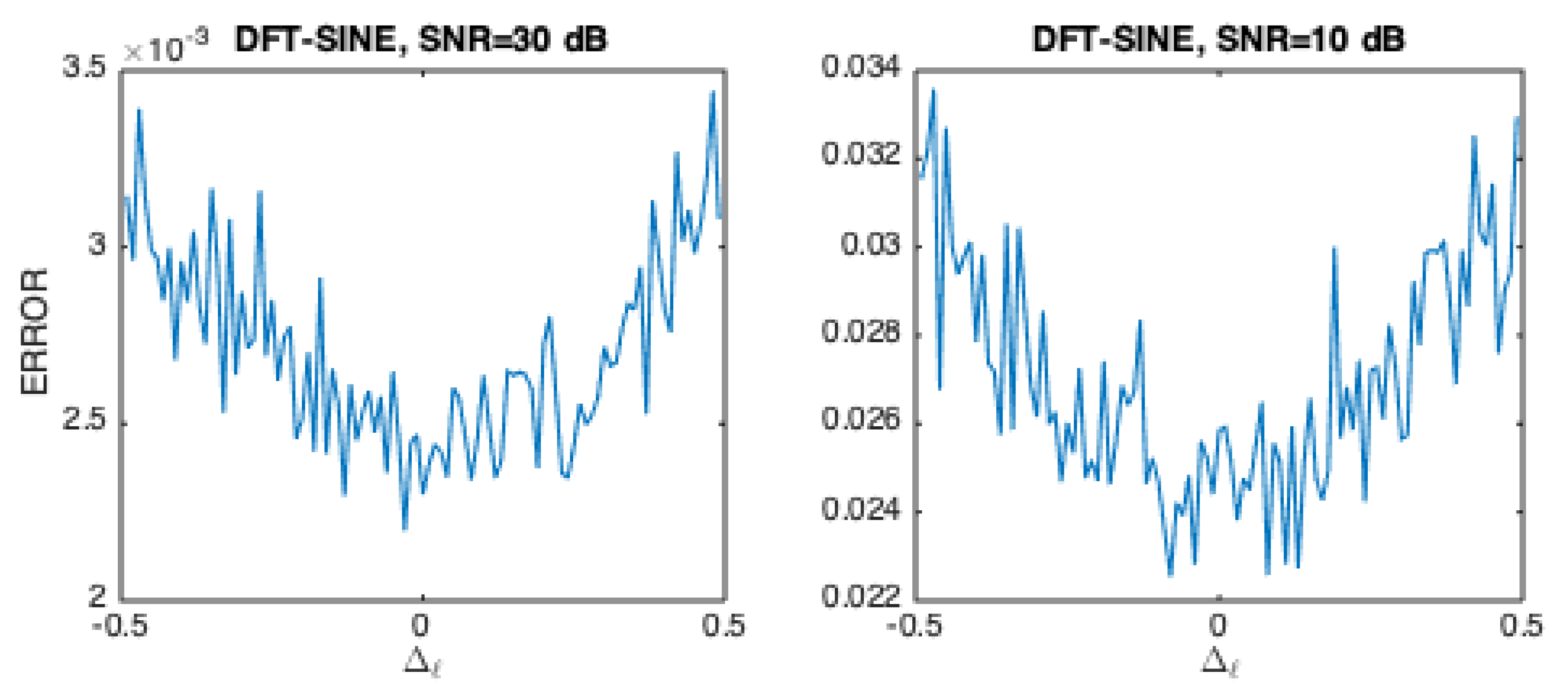Using the same simulation conditions, and using the same phase estimation function (Equation (10)), we obtain the cumulative phase estimation error results that are illustrated in Figure 7.

When compared to the results in Figure 5, it can be concluded that phase estimation appears to be more accurate when the Sine window is used, especially when the SNR is high, which is a natural consequence of the smaller leakage caused by this window. Results are similar if the shifted Hanning window is considered instead. As we shall see in Section 2.5, more informative conclusions will emerge from a study of the phase estimation error variance.

2.3. ODFT and the Rectangular window

An N-point DFT corresponds to a filter bank whose N sub-bands are `evenly stacked’, i.e., their center frequencies correspond to

\frac{π}{N} (2 k)

k = 0, 1, \dots, N - 1

. An alternative option involves `oddly stacked’ sub-bands, i.e., their center frequencies correspond to

\frac{π}{N} (2 k + 1)

k = 0, 1, \dots, N - 1

. In this case, the time-frequency transformation results as

X [k] = \sum_{n = 0}^{N - 1} x [n] w [n] e^{- j \frac{2 π}{N} n (k + \frac{1}{2})}, k = 0, 1, \dots, N - 1,

(18)

and is known as Odd-frequency DFT, or just Odd-DFT [19]. We also abbreviate this designation to ODFT. Although it is not too much different from the basic DFT, it has several advantages that make it preferable in certain contexts. For example, assuming that the window is real-valued and symmetric, and if

x [n]

is also real-valued, then the conjugate-symmetric property is expressed as

X [k] = X^{*} [N - 1 - k]

k = 0, 1, \dots, N / 2 - 1

, i.e., only

N / 2

values of

X [k]

are unique, instead of

N / 2 + 1

, as in the case of the DFT. This subtle difference facilitates, for example, signal modification by avoiding the special cases of the DFT corresponding to

k = 0

and

k = N / 2

. For example, the ODFT facilitates signal integration in the frequency-domain because none of the sampled frequencies is zero, which avoids the singularity that occurs in the case of the DFT when

k = 0

[20].

When the sinusoidal signal (5) is multiplied by the Rectangular window (7) and the result is ODFT transformed, then the relevant maximum that exists in the magnitude spectrum and that occurs for

k = k_{ℓ}

, is given by

X [k_{ℓ}] \approx \frac{A}{2} e^{j (ϕ_{ℓ} - \frac{π}{2} + π (Δ_{ℓ} - \frac{1}{2}) (1 - \frac{1}{N}))} \frac{sin π (Δ_{ℓ} - \frac{1}{2})}{sin \frac{π}{N} (Δ_{ℓ} - \frac{1}{2})} .

(19)

However, in this case, the fact that the sampled frequencies of the ODFT rotate by

π / N

relative to those of the DFT, makes that the phase can be estimated from the same local maximum as long as

Δ_{ℓ} \in [0.0, 1.0 [

. This means that the illustration of the spectral magnitudes surrounding the local maximum in Figure 4 is also valid in this context, except that it applies to this new

Δ_{ℓ}

range. Under this assumption, from (19) we obtain

∠ X [k_{ℓ}] = ϕ_{ℓ} - \frac{π}{2} + π (Δ_{ℓ} - \frac{1}{2}) (1 - \frac{1}{N})

, which leads to

ϕ_{ℓ} = ∠ X [k_{ℓ}] + \frac{π}{2} - π (Δ_{ℓ} - \frac{1}{2}) (1 - \frac{1}{N}) .

(20)

As in the previous two subsections, we can avoid the dependence on the prior estimation of

Δ_{ℓ}

by considering a time reference corresponding to the group delay of the window, which implies adding

ω_{ℓ} τ

to (20), i.e.,

\begin{matrix} {\hat{ϕ}}_{ℓ} & = & ∠ X [k_{ℓ}] + \frac{π}{2} - π (Δ_{ℓ} - \frac{1}{2}) (1 - \frac{1}{N}) + ω_{ℓ} τ \\ = & ∠ X [k_{ℓ}] + π (1 - \frac{1}{2 N}) + π k_{ℓ} (1 - \frac{1}{N}) . \end{matrix}

(21)

Although this result is different from the one discussed in the previous two subsections, it reveals the same important property that phase estimation depends on the spectral bin index of the local maximum in the magnitude spectrum, instead of the fractional frequency

Δ_{ℓ}

, which adds robustness to the phase estimation process. Figure 8 shows the cumulative phase estimation error that results from (21) when the test conditions are the same as those that are considered in Section 2.1 and Section 2.2.

When the results in Figure 8 are compared to the results in Figure 5, it can be seen that no major differences exist, as expected (essentially because the same window is used), although the results in Figure 8 are slightly better. This is explained by the fact that the ODFT implicitly performs a small frequency modulation (i.e., an upshift in frequency by

π / N

) of the input signal, which improves the frequency separation between the two Dirichlet kernels, and this slightly reduces the mutual interference due to leakage.

2.4. ODFT and the Sine and shifted Hanning Windows

When we compute the N-point ODFT (Equation (18)) of the sinusoid (5) and take for

w [n]

the Sine window (Equation (12)), a relevant local maximum exists in the magnitude spectrum

| X [k_{ℓ}] |

k = k_{ℓ}

whose spectral coefficient can be approximated by

X [k_{ℓ}] \approx \frac{A}{4} e^{j (ϕ_{ℓ} - \frac{π}{2} + π (Δ_{ℓ} - \frac{1}{2}) (1 - \frac{1}{N}))} H (Δ_{ℓ}),

(22)

where

H (Δ_{ℓ}) = \frac{sin π Δ_{ℓ}}{sin \frac{π}{N} Δ_{ℓ}} + \frac{sin π (Δ_{ℓ} - 1)}{sin \frac{π}{N} (Δ_{ℓ} - 1)} .

(23)

In the case of the shifted Hanning window, the local maximum in the magnitude spectrum can be approximated by

X [k_{ℓ}] \approx \frac{A}{4} e^{j (ϕ_{ℓ} - \frac{π}{2} + π (Δ_{ℓ} - \frac{1}{2}) (1 - \frac{1}{N}))} G (Δ_{ℓ}),

(24)

where

G (Δ_{ℓ}) = 2 \frac{sin π (Δ_{ℓ} - \frac{1}{2})}{sin \frac{π}{N} (Δ_{ℓ} - \frac{1}{2})} + \frac{sin π (Δ_{ℓ} + \frac{1}{2})}{sin \frac{π}{N} (Δ_{ℓ} + \frac{1}{2})} + \frac{sin π (Δ_{ℓ} - \frac{3}{2})}{sin \frac{π}{N} (Δ_{ℓ} - \frac{3}{2})} .

(25)

Given that both (23) and (25) are always positive when

Δ_{ℓ} \in [0.0, 1.0 [

, they do not affect phase in this range of

Δ_{ℓ}

Equations (22) and (24) show that the phase of the ODFT spectral line corresponding to the local maximum is the same as that already found for the ODFT and Rectangular window combination. As noted previously, this is expected given that all three windows share the same linear-phase property, and the same group delay. As a consequence, phase can be estimated using Equation (21) although it remains true that the quality of the phase estimation depends on the specific near-end and far-end leakage properties of each window.

Taking the Sine window as an example, Figure 9 shows the cumulative phase estimation error arising from phase estimation according to (21) and taking into consideration the processing conditions in this section.

When the results in Figure 9 are compared to the results in Figure 7, our results here are slightly better despite the fact that both relate to the same window. As pointed out in the previous section, this is due to the fact that the ODFT promotes a wider separation between Dirichlet kernels, which means that leakage effects become weaker. Results for the shifted Hanning window do not differ significantly.

Matlab code is available (estimatePHASE_ODFT_sine.m) that creates results and displays Figure 9 .

2.5. Bias and Variance of the Phase Estimation Error

We complete this section (Section 2) with an assessment of the bias, and of the variance of the phase estimation error that results from the estimators that are explained in Section 2.1 (Equation 10), and in Section 2.4 (Equation (21)). Bias is computed using

m e a n {ϕ - \hat{ϕ}}

. Variance is computed using

v a r {ϕ - \hat{ϕ}}

, and and we take as a reference the Cramér-Rao lower bound (CRLB) for an unbiased phase estimator [21]. Assuming that both magnitude and frequency of the sinusoid are known –which is true in our simulations–, this CRLB is given by

var {ϕ - \hat{ϕ}} = \frac{2 σ^{2}}{N A^{2}},

(26)

where

σ^{2}

is the variance of real-valued white Gaussian noise.

As the results in Figure 5 and in Figure 9 make clear, the phase estimation error is influenced by –although it does not directly depend on– the fractional frequency

Δ_{ℓ}

, which we represent in this context simply as

Δ

given that we are considering just one sinusoid. Hence, we evaluate the bias and variance of the phase estimation error in two almost extreme situations: when

Δ = - 0.49

or when

Δ = 0.00

in the case of the estimator given by Equation (10), and when

Δ = 0.01

or when

Δ = 0.5

in the case of the estimator defined by Equation (21). In our simulations,

N = 128

and

ℓ = 13

. Results are obtained when the SNR varies from 0 dB to 30 dB in steps of 2.5 dB. For each particular SNR value, the bias and variance of the phase estimation error are computed when

ϕ

varies between

- π

and

+ π

in 200 steps and, at each step, stable statistics are reached after 100 Monte Carlo runs accounting for noise contamination.

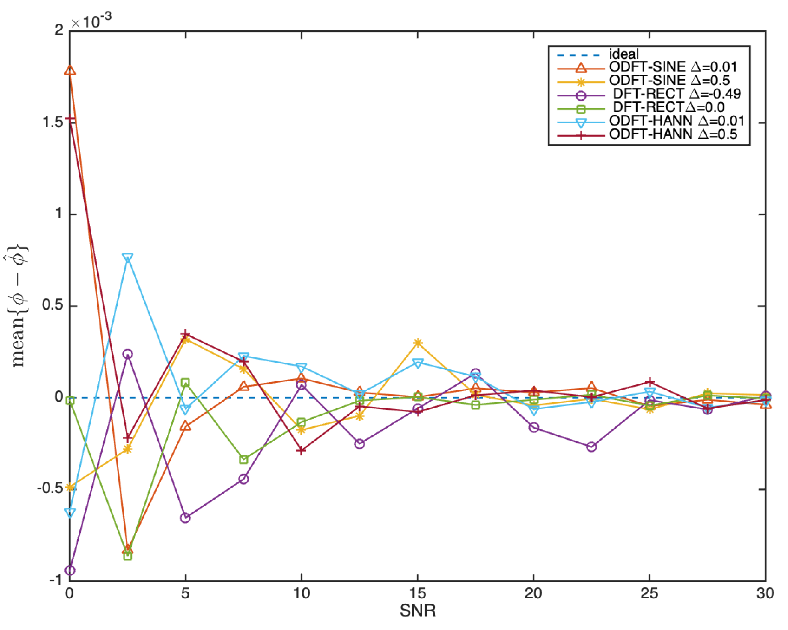
Figure 10 displays representative results regarding bias. Results reveal that in all six cases bias reduces as the SNR increases, as expected. However, there is not a specific combination of DF-based filter bank and window that stands out. This remains true even after repeating the simulations, although a relative degradation can be observed for the tested Rectangular window context (i.e., DFT filter bank and Rectangular window) under more adverse

Δ

conditions (i.e., when

Δ

approaches -0.5 ou 0.5), which is easily explained by the poor leakage characteristics of the Rectangular window.

In general, it can be concluded that bias is fairly low, in the order or less than 1E-3 radians for SNR equal to or larger than 2.5 dB. This represents less than 0.016% of the

2 π

dynamic range.

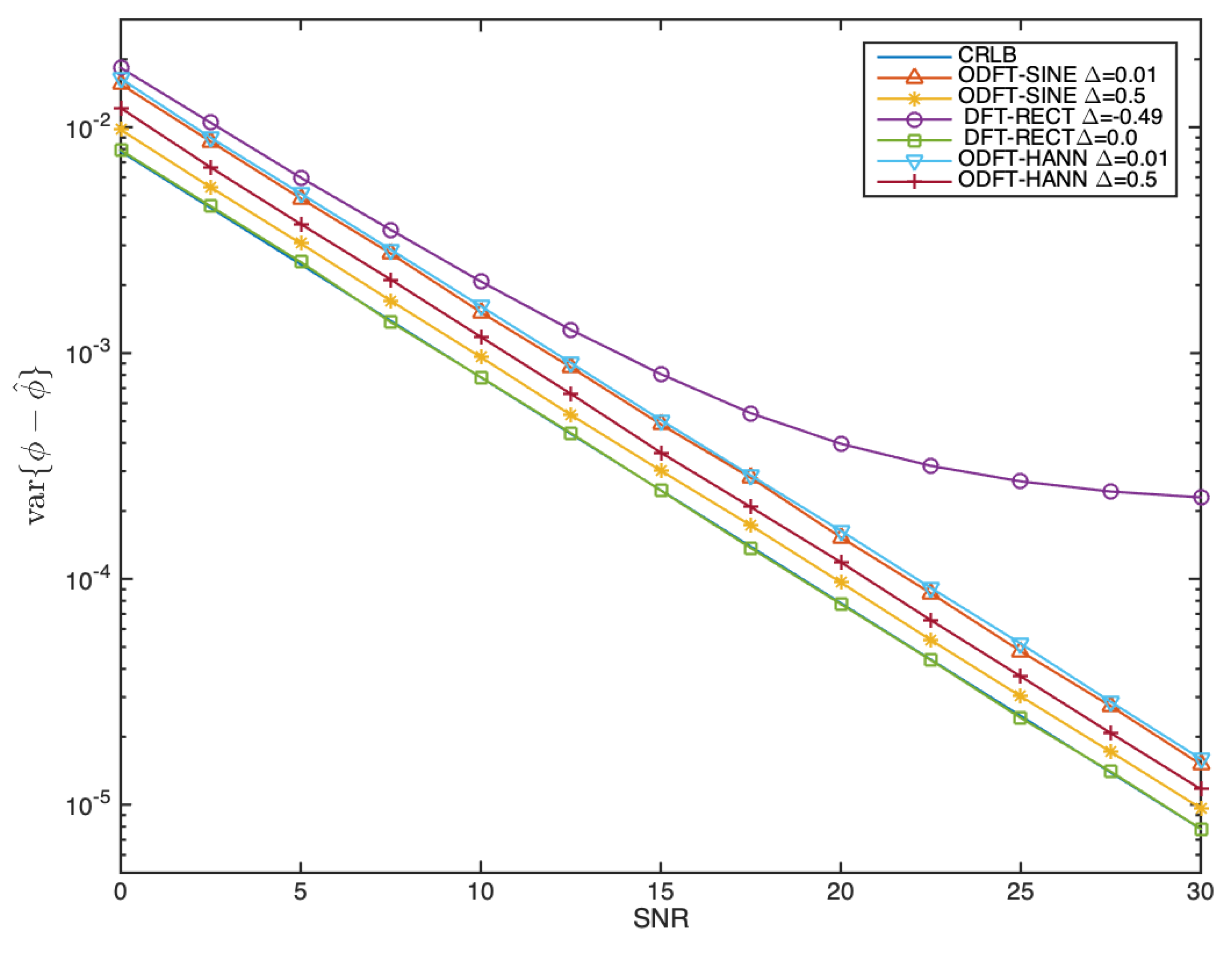
The most significant results regard estimation error variance and are shown in Figure 11.

It is an interesting and somewhat unexpected outcome that the Rectangular window gives rise to the best results when the tested

Δ

conditions are more favorable (i.e., when

Δ = 0.0

), and to the worst results when the tested

Δ

conditions are more adverse (i.e., when

Δ = - 0.49

). In the former case, the performance reaches the CRLB because in that ideal case there is no leakage, as already noted at the end of subSection 2.1, which means that the error variance is entirely due to the noise contamination. It should be noted that in practice, this rarely happens with real-world, natural, signals as it is quite unlikely that the analyzed frequencies are exactly aligned with the center frequencies of the sub-bands of the DFT-based filter bank. In the latter case, the performance shown by the same estimator is quite poor, which reveals that, in that case, leakage effects due to the Rectangular window are quite strong, as the results in Figure 5 and Figure 8 anticipated. In particular, the performance becomes asymptotic when the SNR exceeds 10 dB, which is commensurate with the known main-to-side lobe attenuation of the Rectangular window, in the order of 13 dB [13].

The performance of the Sine and shifted Hanning windows fall in between the two extreme cases associated with the Rectangular window. In particular, for the same DFT-based filter bank and

Δ

conditions, the error variance performance of the Sine window clearly exceeds that of the shifted Hanning window in the sense that a closer approximation to the CRLB is reached. This is more evident under the more favorable

Δ

test conditions (e.g., when

Δ = 0.5

), than under the more adverse

Δ

test conditions (e.g., when

Δ = 0.01

A possible explanation may be linked to the relationship between the main lobe width of the magnitude of the frequency responses of those two windows, the relative prominence of the spectral coefficients inside that main lobe and associated with the discrete-frequencies defining the different DFT channels (or sub-bands), and the near-end and far-end leakage properties of each window.

The most impactful implication of these results is that under more general test conditions, the phase estimation error performance of the Sine window is not only closer to the CRLB, but also offers a lower deviation when signal conditions are more adverse. For these reasons, it can be considered that the performance of the Sine window is better behaved and, thus, it will be used in the remainder of this paper.

As a final note, it should be highlighed that changing ℓ in the simulations produces a marginal effect on the results. In particular, when

ℓ = N / 4 - 1

, which corresponds to the `sweet spot’ given that leakage effects are minimized, results do not differ appreciably from those in Figure 11. The Matlab file generating and displaying the results in Figure 10 and Figure 11 is available (CRLBphivar.m) such that other combinations of parameters can be tried.

3. An Interpretable Time-Shift Invariant Harmonic Phase Model

In this section, we take advantage of phase estimation of individual sinusoids using the signal representation in a discrete-time and discrete-frequency Fourier domain, as it was discussed in the previous section, especially SubSection 2.4. The objective is to identify a vertical harmonic phase model that is time-shift invariant, and that can be approximated by a simple parametric model.

In our development in this section, we use the deterministic part of (1) taking into consideration the harmonic relationship given by (2). Thus, in our analysis, we use

\begin{matrix} x (t) & = & \sum_{ℓ = 0}^{L - 1} A_{ℓ} sin ((ℓ + 1) Ω_{0} t + ϕ_{ℓ}) \\ = & \sum_{ℓ = 0}^{L - 1} A_{ℓ} sin ((ℓ + 1) Ω_{0} (t + t_{ℓ})) \\ = & A_{0} sin (Ω_{0} (t + t_{0})) + v (t), \end{matrix}

(27)

where

t_{ℓ}

represents the starting delay of harmonic ℓ, and

v (t)

represents all harmonics above the fundamental frequency. If

Ω_{0} = 2 π / T_{0}

, where

T_{0}

is the fundamental period, i.e., the reciprocal of the fundamental frequency (

F_{0}

), a convenient manipulation of

v (t)

leads to

\begin{matrix} v (t) & = & \sum_{ℓ = 1}^{L - 1} A_{ℓ} sin ((ℓ + 1) Ω_{0} (t + t_{ℓ})) \\ = & \sum_{ℓ = 1}^{L - 1} A_{ℓ} sin ((ℓ + 1) Ω_{0} (t + t_{0} - t_{0} + t_{ℓ})) \\ = & \sum_{ℓ = 1}^{L - 1} A_{ℓ} sin ((ℓ + 1) Ω_{0} (t + t_{0}) + 2 π \frac{t_{ℓ} - t_{0}}{T_{0} / (ℓ + 1)}) \\ = & \sum_{ℓ = 1}^{L - 1} A_{ℓ} sin ((ℓ + 1) Ω_{0} (t + t_{0}) + 2 π {NRD}_{ℓ}), \end{matrix}

(28)

where

{NRD}_{ℓ}

denotes the Normalized Relative Delay of harmonic ℓ, and is defined as

{NRD}_{ℓ} = \frac{t_{ℓ} - t_{0}}{T_{0} / (ℓ + 1)} = \frac{ϕ_{ℓ} - (ℓ + 1) ϕ_{0}}{2 π} .

(29)

{NRD}_{ℓ}

expresses the difference between the starting delay of harmonic ℓ, and the starting delay (i.e., the onset) of the fundamental frequency, which is further normalized by the period of harmonic ℓ[22]. Therefore, in its most intuitive interpretation, NRD can be taken modulo 1, which means that

{NRD}_{ℓ} \in [0.0, 1.0 [

. Equation (29) allows two other important conclusions. First, by definition,

{NRD}_{0} = 0

. This means that, by definition, the NRD phase-related feature is intrinsically time-shift invariant. Second, as the second part of (29) highlights, the NRD does not depend on the fundamental frequency. Therefore, we may rewrite (27) as

x (t) = \sum_{ℓ = 0}^{L - 1} A_{ℓ} sin ((ℓ + 1) Ω_{0} (t + t_{0}) + 2 π {NRD}_{ℓ}),

(30)

which highlights the fact that, in terms of phase, all harmonics can be expressed as a part that depends on the time-varying phase of the fundamental frequency, and on its starting phase, and another part, the NRD, that is time-shift invariant. Thus, the NRD acts as a holistic harmonic phase model that is identified in Figure 2 as PM.

Other harmonic phase descriptors that are similar to NRD were proposed by Stylianou in 1996 (phase envelope [23]), Di Federico in 1998 [24], and Saratxaga in 2009 (Relative Phase Shift -RPS [25]).

An inspiring metaphor from Nature and elucidating on the meaning of NRD is depicted in Figure 12.

Each bird in the flock formation is like a harmonic in a harmonic structure, and the dynamics of the wings of the former, is like the dynamics of the phase rotation of the later. The NRD feature represents a shift-invariant harmonic phase structure, similarly to the space-invariant bird formation structure of the flock that is represented by the line connecting the birds in the upper branch of the flock. Ultimately, the whole flock flying dynamics are governed by the position and wing evolution of the leading bird in the flock, inasmuch as the whole harmonic dynamics are governed by the phase evolution of the fundamental frequency in the harmonic structure.

On the other hand, since the NRD inherits the properties of phase, then phase wrapping and phase unwrapping also apply to NRD feature vectors. It should be noted, however, that in this case, phase (un)wrapping is vertical, meaning that it is performed along the frequency axis, as apposed to the time axis, which is by far the most common use of phase (un)wrapping operations.

As a summary, the NRD captures the vertical phase structure (i.e., along the frequency axis) of all the harmonic sinusoids, which just depends on the waveform shape of the periodic signal they define. It should be stressed that when (vertical) harmonic magnitude and (vertical) harmonic phase structure are combined, they uniquely define the waveform shape of a given periodic signal, independently of its time-shift, and of its fundamental frequency.

In the next three subsections, we take inspiration from [20] in order to demonstrate the practical estimation of three different NRD feature vectors that characterize three different waveforms, all of them emerging from the sawtooth wave.

3.1. NRD Estimation Example Based on the Sawtooth Wave

In this subsection, and throughout the rest of this paper, we use a convenient ground-truth signal that consists in the sawtooth waveform. In order to work with realistic NRD estimation conditions, the fundamental frequency (

F_{0}

) is time-varying, and two levels of noise contamination are considered.

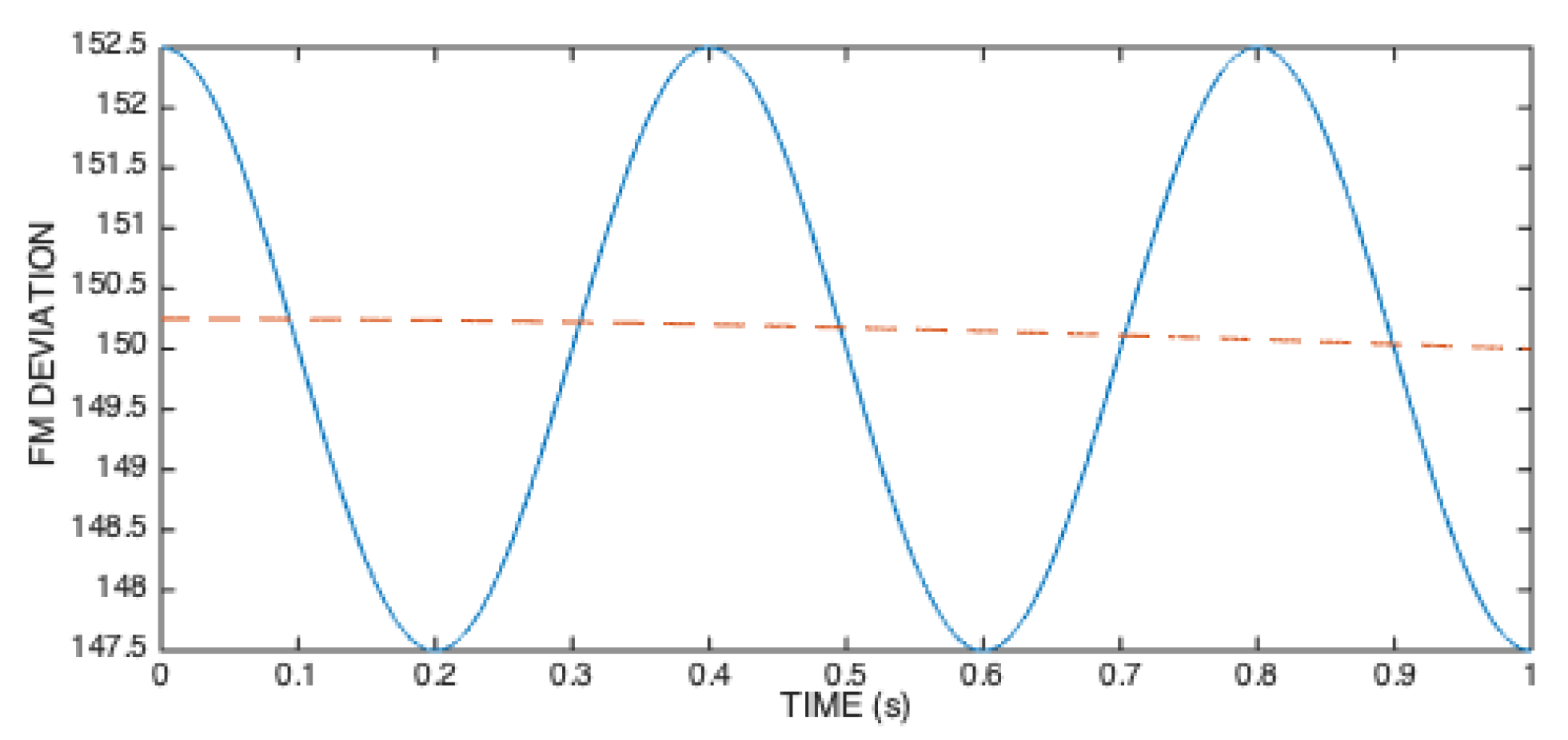
Regarding the time-varying fundamental frequency, we take the average pitch frequency between female and male human speakers, which is around 150 Hz, and subject it to frequency-modulation (FM) as specified in Equation (31).

F_{0} (t) = 150.0 + F M cos (2 π \cdot F M \cdot t)

(31)

In our simulations, we consider two FM values: FM=2.5 Hz, and FM=0.25 Hz. These cases of maximum frequency deviation around the mean are illustrated in Figure 13.

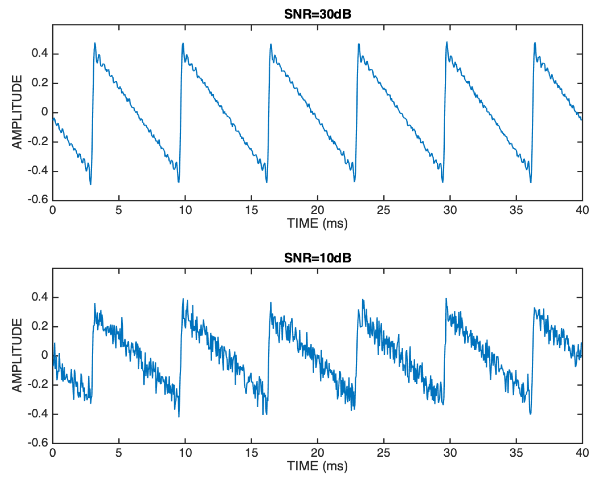
The sawtooth waveform is illustrated in Figure 14 for two noise contamination scenarios that we consider in our simulations: when it is mild (SNR=30 dB), and when it is strong (SNR=10 dB).

In our simulations, the sampling frequency is 22050 Hz, the duration of the test signals is 1 s, and the number of harmonics is

L = 20

. Time-frequency transformation is performed as discussed in Section 2.4, with

N = 1024

, and 50% overlap between adjacent frames.

Using standard Fourier analysis [12], it is easy to show that the starting phases of the sawtooth waveform in (1) are all

ϕ_{ℓ} = 0, ℓ = 0, 1, \dots, L - 1

, which means that the harmonic phase structure is simply given by

{NRD}_{ℓ} = 0, ℓ = 0, 1, \dots, L - 1

. On the other hand, the normalized harmonic magnitude ratios that express the harmonic magnitude structure of the sawtooth waveform are simply given by

A_{ℓ} / A_{0} = \frac{1}{ℓ + 1}, ℓ = 0, 1, \dots, L - 1 .

(32)

Given that we have access to the ground-truth value of the instantaneous fundamental frequency, as specified by (31), and by adopting the frequency front-end that is assumed in SubSection 2.4 (i.e., ODFT and Sine window), we may easily obtain the ground-truth spectral indices (

k_{ℓ}

) of all 20 local maxima in the ODFT magnitude spectrum. These indices allow us to estimate the individual harmonic phases as specified by (21) and, from these, we estimate the NRD coefficients for all harmonics. By vertically unwrapping these coefficients, we obtain interpretable representations which are amenable to simple parametric modeling.

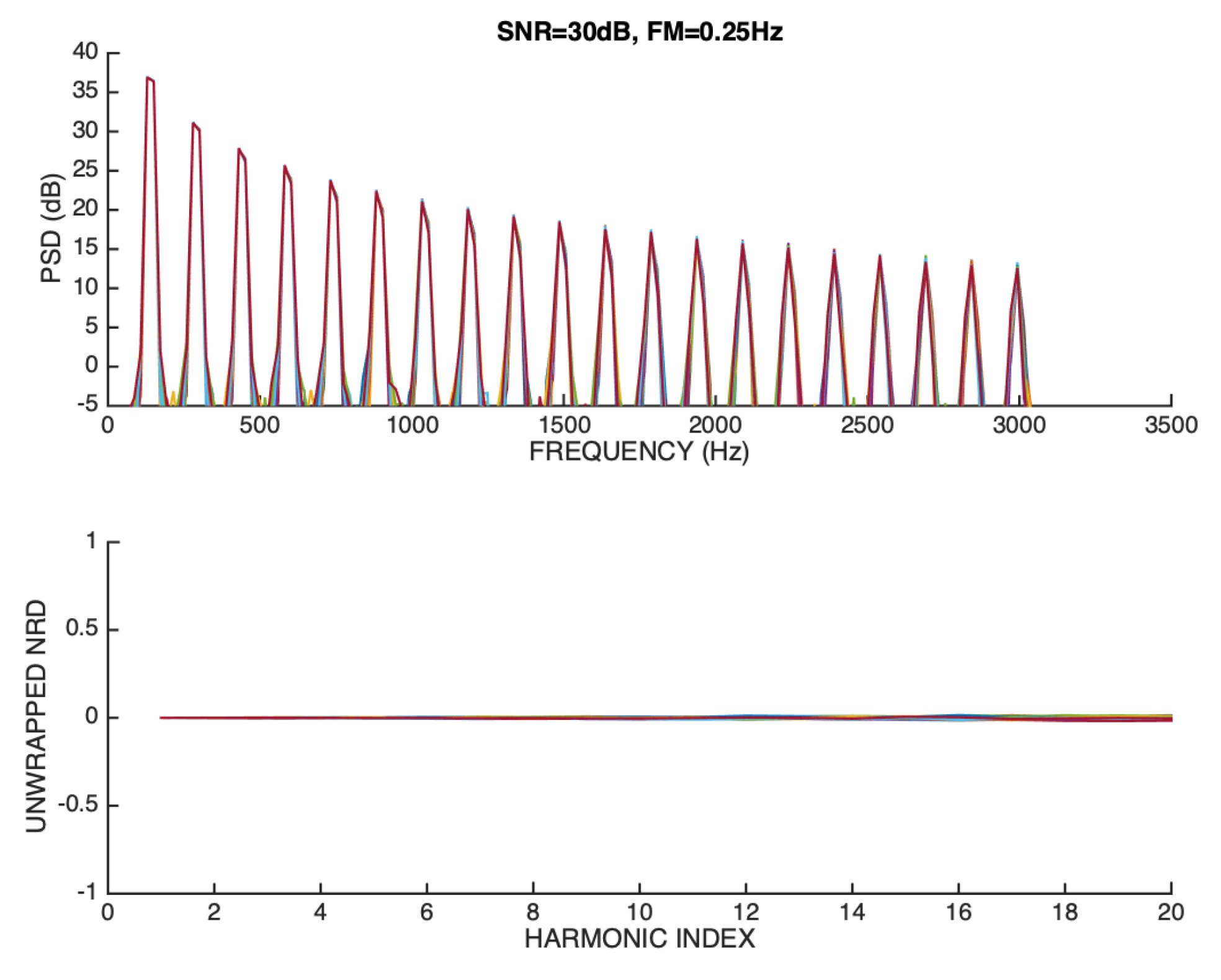
Figure 15 represents an overlay of the magnitude spectra and unwrapped NRD vectors of our test signal when the maximum frequency deviation around the mean is 0.25 Hz, and the SNR is 30 dB.

It can be seen that, as expected, the magnitude spectra are aligned in a very consistent way because the FM modulation is small, and the SNR is high. On the other hand, it can also be seen that the unwrapped NRD vectors are also very closely aligned to the ideal ground-truth model (

{NRD}_{ℓ} = 0, ℓ + 1 = 1, 2, \dots, 20

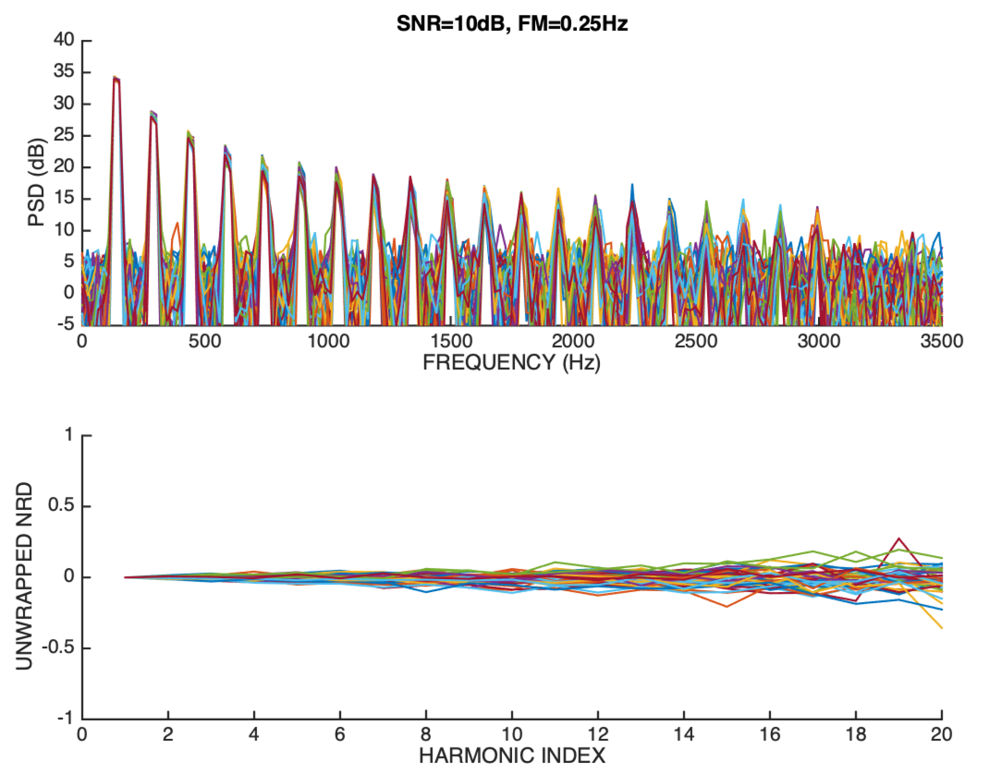
Figure 16 repeats the overlay representation when the SNR is 10 dB. It can be seen that higher-order harmonics are strongly contaminated by noise, especially when their magnitude approaches the noise floor, which adversely impacts the accuracy of phase estimation.

This is clear in Figure 16 because the unwrapped NRD vectors deviate more from the ideal ground-truth model as the harmonic order increases. Still, their average follows the correct model.

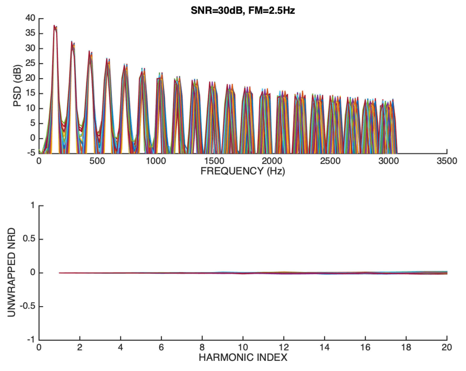
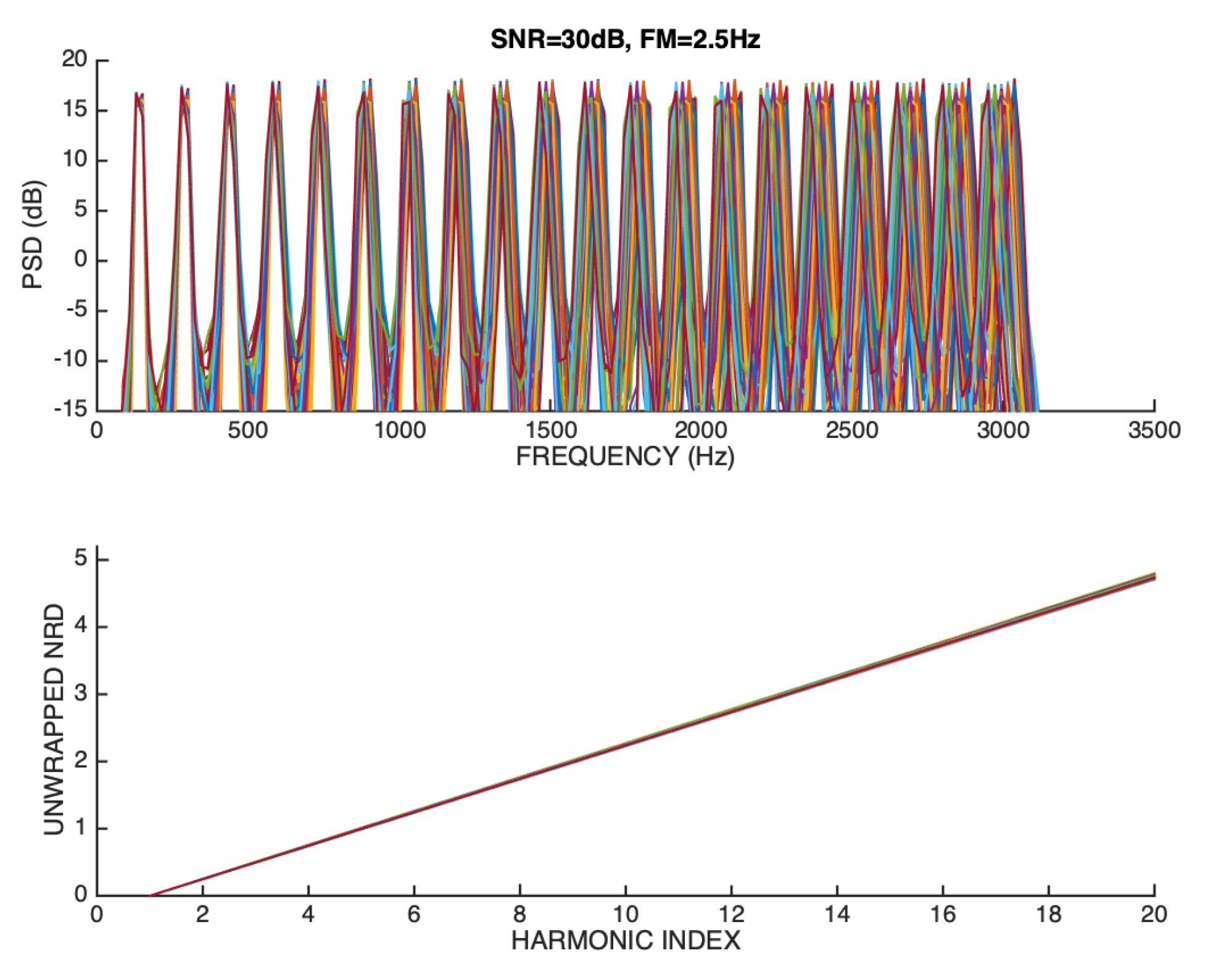
Figure 17 represents the results when SNR=30 dB and FM=2.5 Hz.

It can be seen that, in this case, the blurred aspect of higher order harmonics in the magnitude spectrum is a natural consequence of the fact that the frequency deviation is proportional to the harmonic order. In particular, for

ℓ = 19

, the maximum frequency deviation around the mean is 50 Hz, which represents

1 / 3

of the average fundamental frequency. It can be confirmed that in spite of the frequency modulation, the dispersion on the unwrapped NRD vectors is quite small, and quite comparable with the one that is observed in Figure 15, in which the frequency modulation is negligible. This relevant experimental outcome unequivocally confirms that the NRD phase-related feature is intrinsically independent of the fundamental frequency. In other words, the stability of the estimated unwrapped NRD vectors reflects mainly the fact that the waveform shape of the periodic signal that is observed in each frame of the signal does not change appreciably.

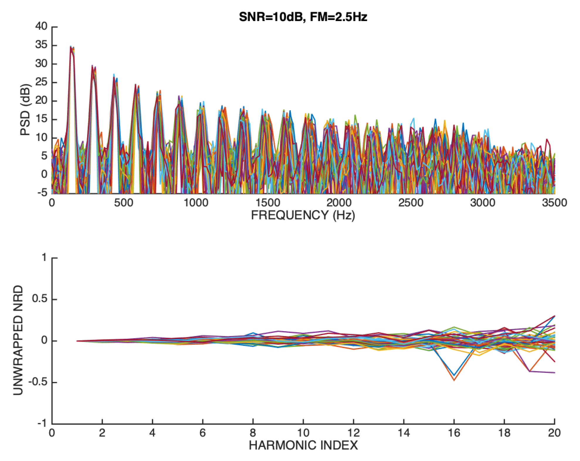
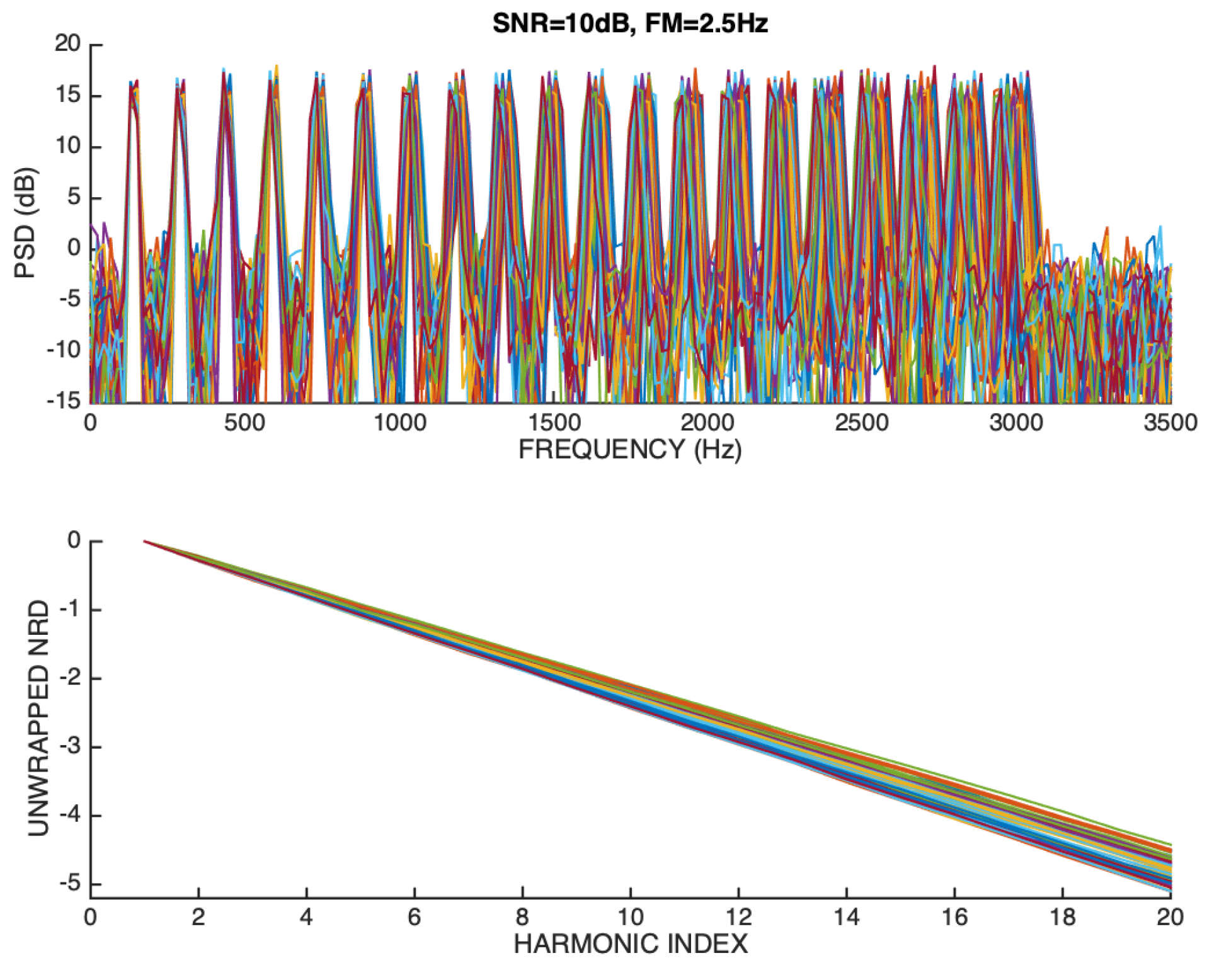
When FM=2.5 Hz and SNR=10 dB, new results are obtained that are represented in Figure 18.

It is easy to anticipate from the spectral magnitude representation that the strong noise influence, when it is allied to the significant frequency deviation of high-order harmonics, paves the way for serious difficulties in phase estimation, which is reflected on the substantial deviation of the unwrapped NRD vectors relative to the ideal ground-truth model. In particular, phase estimation errors cause the phase unwrapping algorithm to introduce sudden jumps of 0.5 on certain unwrapped NRD vectors. However, mitigating strategies could be easily adopted that could detect and avoid such jumps.

The Matlab code that generates signals and creates the overlay representations, as illustrated in previous figures, is available (

g e r a w a v_v 4 . m

), which facilitates that results for other simulation parameters be obtained.

3.2. NRD estimation examples based on the sawtooth wave derivative

The sawtooth wave is defined by (27) with

ϕ_{ℓ} = 0, ℓ = 0, 1, \dots, L - 1

, i.e.

x (t) = \sum_{ℓ = 0}^{L - 1} A_{ℓ} sin ((ℓ + 1) Ω_{0} t),

(33)

where

A_{ℓ} / A_{0}

is defined by (32). Its derivative is obtained as

\begin{matrix} \frac{d}{d t} x (t) & = & \sum_{ℓ = 0}^{L - 1} A_{ℓ} (ℓ + 1) \frac{2 π}{T_{0}} cos ((ℓ + 1) Ω_{0} t + ϕ_{ℓ}) \\ = & \frac{2 π A_{0}}{T_{0}} \sum_{ℓ = 0}^{L - 1} sin ((ℓ + 1) Ω_{0} t + \frac{π}{2}), \end{matrix}

(34)

and its negative derivative is

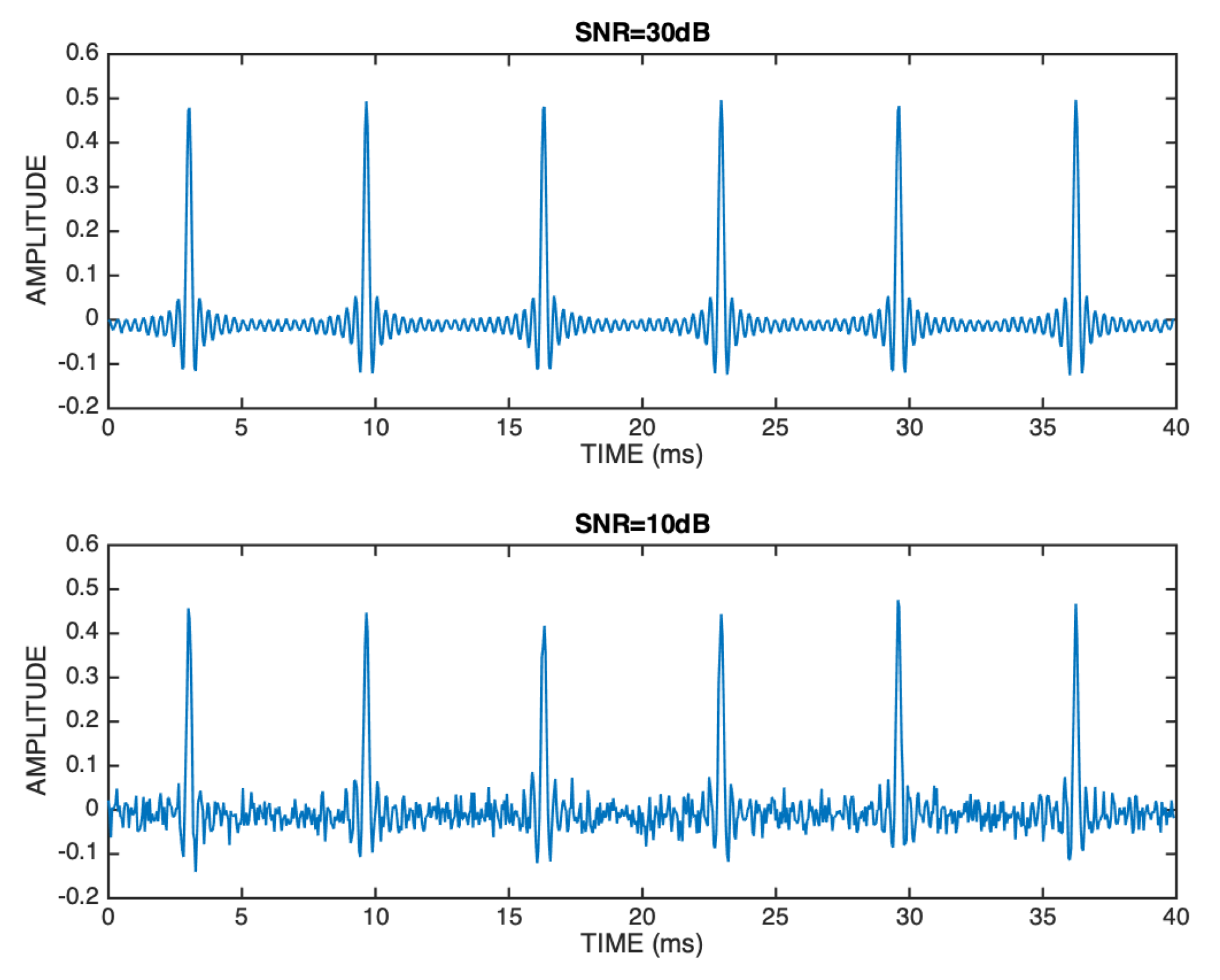
- \frac{d}{d t} x (t) = \frac{2 π A_{0}}{T_{0}} \sum_{ℓ = 0}^{L - 1} sin ((ℓ + 1) Ω_{0} t - \frac{π}{2}) .

(35)

The derivative of the sawtooth wave is illustrated in Figure 19 after magnitude normalization and after it has been contaminated by white Gaussian noise at 30 dB and 10 dB SNR.

In the case of the sawtooth wave derivative, according to (34), it results that

ϕ_{ℓ} = π / 2, ℓ = 0, 1, \dots, L - 1

and, in the case of the negative of the sawtooth wave derivative,

ϕ_{ℓ} = - π / 2, ℓ = 0, 1, \dots, L - 1

. As a consequence, using (29), in the first case we obtain

{NRD}_{ℓ} = \frac{\frac{π}{2} - (ℓ + 1) \frac{π}{2}}{2 π} = - \frac{ℓ}{4}, ℓ = 0, 1, \dots, L - 1,

(36)

and, in the second case, we obtain

{NRD}_{ℓ} = \frac{- \frac{π}{2} + (ℓ + 1) \frac{π}{2}}{2 π} = \frac{ℓ}{4}, ℓ = 0, 1, \dots, L - 1 .

(37)

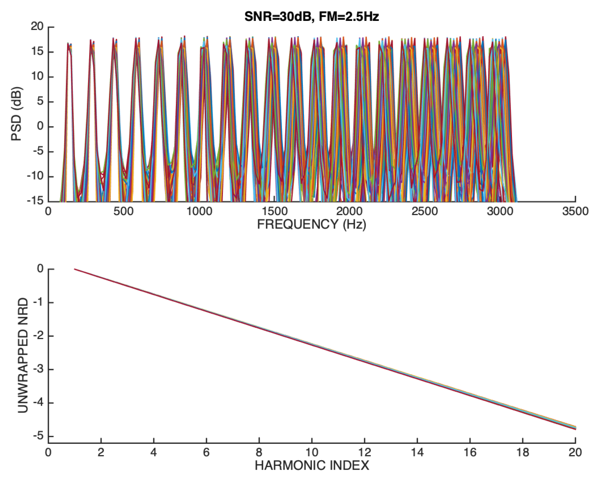
We illustrate in Figure 20 the experimental results regarding the sawtooth wave derivative when FM=2.5 Hz and SNR=30 dB.

It can be confirmed that the unwrapped NRD vectors match quite precisely the ground-truth NRD model according to (36). This model is a simple first-order equation whose value is

NRD = - 4.75

for

ℓ = 19

. This good match happens despite the fact that FM modulation is substantial, especially for higher order harmonics. As noted in the previous subsection, this is a consequence of the fact that NRD is intrinsically independent of the fundamental frequency.

Similar conclusions are obtained in the practical estimation of the negative of the sawtooth derivative signal that is subject to FM modulation and noise contamination, as in the previous case. The results, when FM=2.5 Hz and SNR=30 dB, are displayed in Figure 21.

It can be confirmed that the estimated unwrapped NRD vectors follow quite closely the ground-truth NRD model according to (37) and reaches

NRD = 4.75

for

ℓ = 19

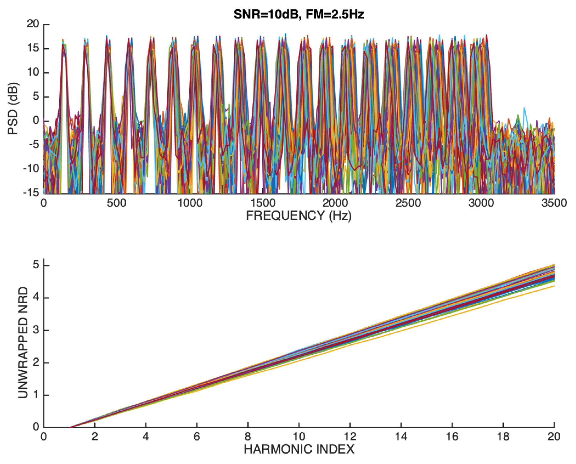
The simulation results for the sawtooth derivative signal, and its negative, when FM=2.5 Hz and SNR=10 dB, are shown in Figure 22, and in Figure 23, respectively.

It can be seen that, in both cases, the unwrapped NRD vectors show some dispersion which is mainly caused by the increased noise floor, which affects phase estimation more severely. In any case, even for this poor SNR level, there are no drastic mismatches relative to the ground-truth NRD model that applies to each case.

These examples suggest that the unwrapped NRD can also be used to detect the polarity of harmonic signals.

3.3. NRD Estimation Examples Using Natural Voice Signals

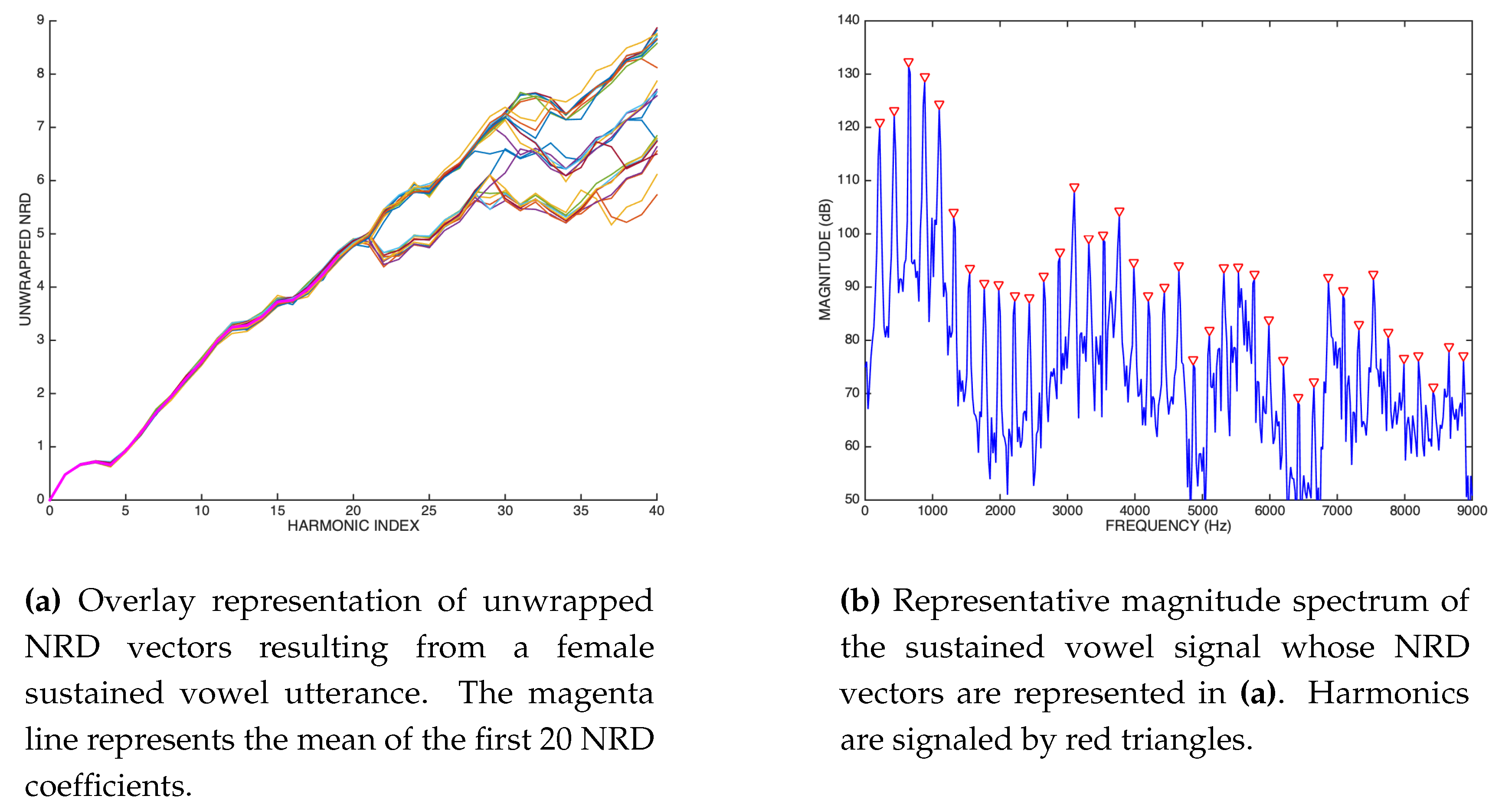
An example of NRD-based analysis with real-world signals involves voiced sounds, i.e., those natural voice sounds that possess a periodic nature as a consequence of the vibration of the vocal folds in the larynx. Figure 24 illustrates an overlay of NRD vectors resulting from a sustained vowel (22050 Hz sampling rate and 1 second long) that was uttered by a female speaker.

It can be seen that NRD vectors are very consistent up to harmonic 22, beyond which a dispersion in the NRD vectors is apparent. This reflects the fact that phase estimation is disturbed after harmonic 22, which can be easily understood by observing one representative magnitude spectrum of the signal, as represented in Figure 24. In fact, it can be confirmed that harmonics 22 and 23, at around 5 kHz, have a very small magnitude, which makes them particularly vulnerable to the noise influence, and leakage effects, which obviously adversely affects phase estimation. In any case, the most important harmonics are correctly characterized in their phase structure, which means reliable NRD models can be built that can be used in parametric-oriented speech processing, as it is illustrated in Figure 2. Our recent research, which assumes this framework, has revealed that when simple NRD modeling is used in the synthesis process, signal reconstruction with transparent audio quality can be achieved, even if the NRD region that exhibits dispersion is replaced by a simple line resulting from extrapolation based on the reliable NRD region (i.e., for which the unwrapped NRD coefficients are consistent) [26,27].

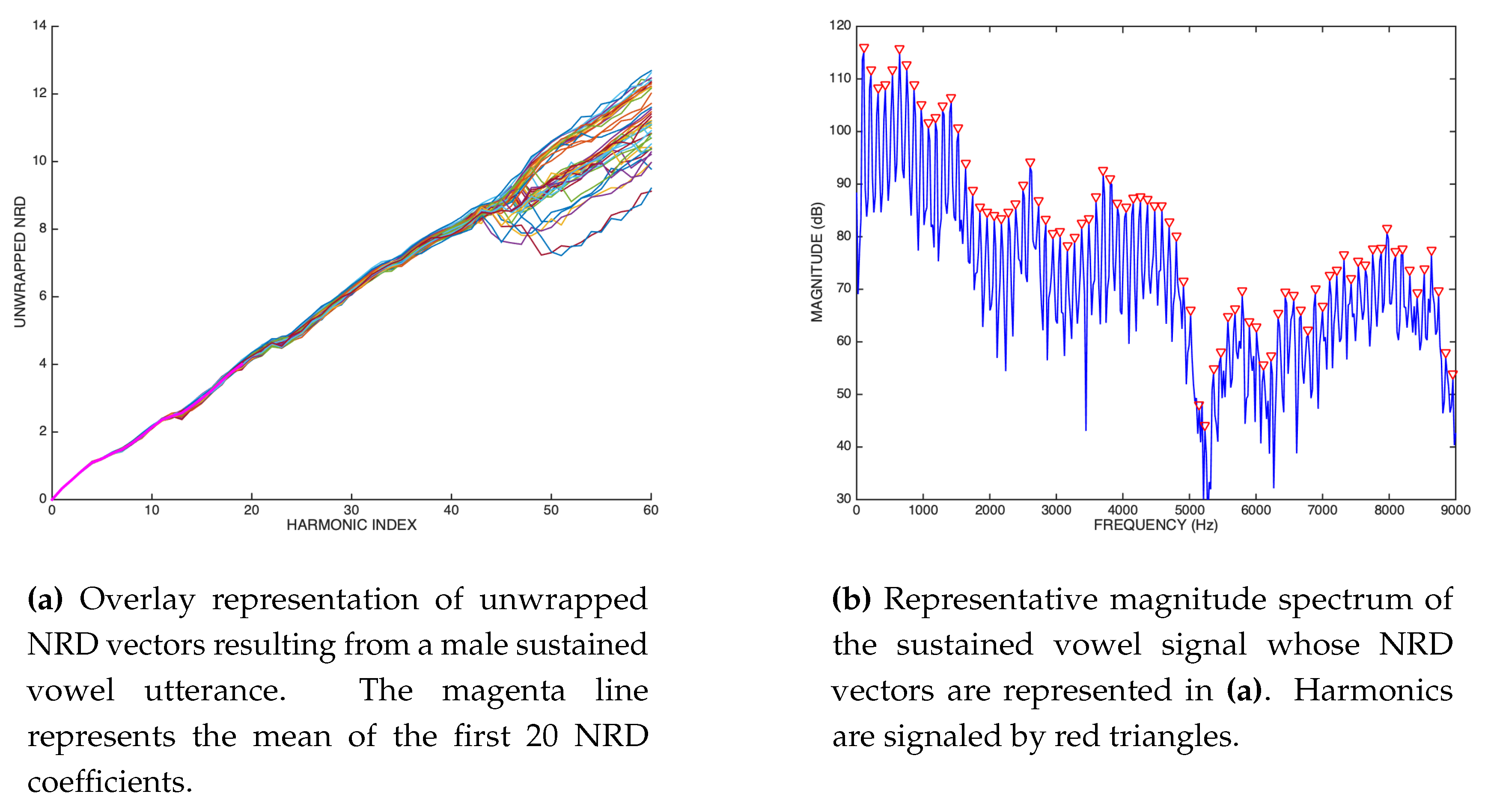
A similar NRD analysis for a sustained vowel that was uttered by a male speaker is illustrated in Figure 25.

It can be seen that the NRD vectors are quite consistent up to harmonics 43-44 that are located around 5 kHz. Figure 25 depicts one representative magnitude spectrum of the vowel signal and it can be confirmed that, similarly to the previous case, the magnitude of those harmonics approaches the noise floor, which makes phase estimation essentially unreliable.

However, the region of the unwrapped NRD vectors that span the most important voice resonances can be reliably modeled. When this is combined with simple modeling of higher-order NRD coefficients though interpolation, very high quality synthesis is achieved which sounds essentially indistinguishable from the original signal [26,27].

Our recent research in parametric voice re-synthesis [27], wideband speech coding [28], and speaker identification [29], highlighted that NRD patterns are idiosyncratic, and that they reflect more strongly the influence of the glottal excitation (i.e., the glottal pulse) than the influence of the vocal tract filter [20,26,30]. The fact that “the vocal tract phase during voicing is not important in achieving naturalness” has been understood already in previous studies [31].

3.4. Demystifying the Phasegram

DFT-based non-parametric spectrum estimation techniques are commonly used to analyze, represent and interpret the spectral properties of a given signal for which no strong assumptions are made. Given that those spectral properties can be characterized in terms of magnitude and phase, typically, 2-D plots and 3-D plots can be used in each case, although only seldomdly in the case of phase representation.

In the case of the magnitude spectrum, also known as periodogram, a 2-D plot is simply obtained as the absolute value of the short-time DFT of a windowed region of the signal as a function of the frequency, as it is illustrated, for example, in Figure 15. The graphical representation can be linear, or logarithmic, either in the horizontal or vertical axis, or in both axes.

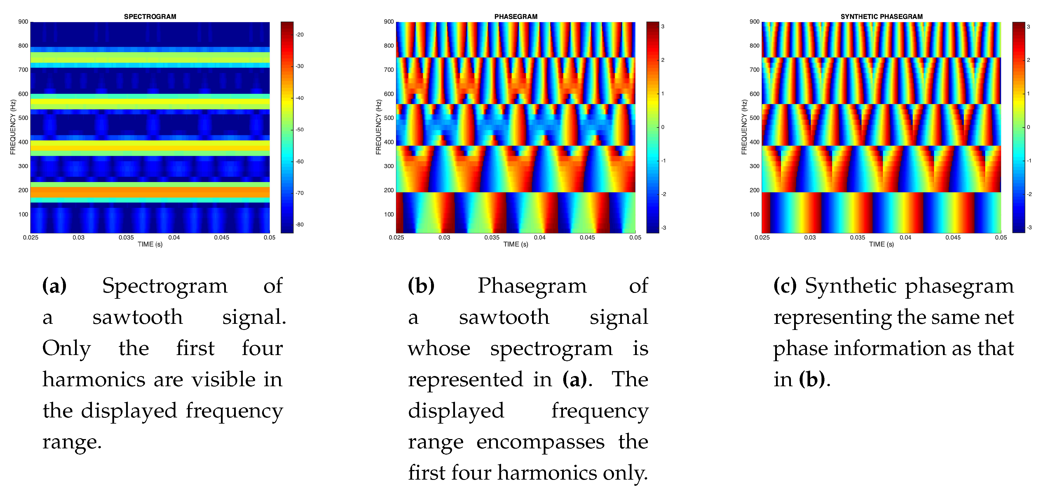
When the goal is to observe how the magnitude spectrum evolves through time, a 3-D representation is created by abutting several magnitude spectra, next to each other, and where a colormap is used to represent Power Spectral Density (PSD). A new magnitude spectrum is obtained by sliding the short-time DFT window over the signal by a certain hop size that, typically, is less than the window length. Such a 3-D representation is known as spectrogram. Usually, the horizontal axis represents time, the vertical axis represents frequency, and the third dimension, which is perpendicular to the time-frequency plane, is represented by a specific color of the colormap denoting a particular PSD range. A simple example is illustrated in Figure 26 that corresponds to the first four harmonics of a sawtooth signal and whose fundamental frequency is

F_{0} = 187.34

Hz.

This particular example allows to conclude that the signal is stationary because the PSD is steady through time. However, since spectrograms are blind to phase, it could happen that the waveform may change its shape with time and may be quite different from the expected sawtooth waveform, albeit the magnitude spectrum remains exactly the same. In other words, the phase structure of the harmonics of the periodic wave may evolve with time. This can be detected by means of another three-dimensional representation called phasegram. The idea of the phasegram is the same as that of the spectrogram, except that the third dimension represents phase instead of power spectral density.

Although colorful and interesting to look at due to the repetitive patterns at different scales, the phasegram is difficult to interpret and, therefore, is not very useful. An evidence of this is that common signal processing-related numerical and graphical environments offer a callable `spectrogram’ function but do not offer a `phasegram’ function.

Here, we want to demystify the phasegram in Figure 26 (and that is valid for a stationary harmonic signal that is not too contaminated by noise) by showing that it is simply an eye-catching representation of the result of phase interpolation at different scales, and where the information that is unique is just the starting phase of the fundamental frequency, and a shift-invariant phase structure such as NRD.

In fact, the different scales are simply caused by the phase rotation of the different harmonics. As expected, the time evolution of the phase is periodic and, relative to the periodicity the fundamental frequency, the time evolution for the second harmonic is two times as fast, three times as fast for the third harmonic, and so on. Thus, according to Equation (30), the phase evolution in time regarding the fundamental frequency is governed by

Ω_{0} (t + t_{0})

and the phase evolution in time for any harmonic ℓ is governed by

(ℓ + 1) Ω_{0} (t + t_{0}) + 2 π {NRD}_{ℓ}

, which highlights that the only phase-related parameters that are unique are the starting phase of the fundamental frequency, and the NRD coefficients. This explains the horizontal phase evolution for a given harmonic and whose local maximum in the magnitude spectrum has index

k_{ℓ}

. The fact that phase changes abruptly at harmonic frequencies between spectral index

k_{ℓ} - 1

and

k_{ℓ}

is explained, for example, with the help of Equation (8). In fact, such phase change is

π (1 - 1 / N)

which, in practical terms (i.e., for large N), consists in a phase inversion. Such a phase inversion does not occur for other spectral indices because, in those cases, the polarity of the real-valued Dirichlet kernel function also inverts, thereby canceling out the phase inversion.

The remaining spectral lines are `passive’ as far as phase is concerned, which means that their phases are the result of a simple vertical interpolation between the phases of the `active’ spectral lines (i.e. those corresponding to local maxima in the magnitude spectrum). In order to illustrate this, we show in Figure 26 a simple replica of the phasegram of Figure 26 and that was built by defining first the horizontal phase evolution of the harmonics, by performing phase rotation by

π (1 - 1 / N)

for

k_{ℓ} - 1

spectral indices, and by performing piecewise vertical phase interpolation for the remaining spectral lines. This helps to reinforce the point –and conclusion– that in the case of stationary periodic signals, the phasegram is a highly redundant graphical representation whose unique information is just the starting phase of the fundamental frequency, and the NRD feature vector.

4. Conclusion

This paper has focussed on a harmonic signal analysis, modeling and processing paradigm that eases significantly the representation, transformation and synthesis of harmonic signals, especially from the point of view of the phase information.

In the first part of the paper, practical DFT-based approaches that build on a filter-bank perspective were discussed for the estimation of the starting phases of individual sinusoids, and their performance was characterized taking into consideration the CRLB for the variance of an unbiased phase estimator. In particular, it was shown that contrarily to harmonic frequency and magnitude estimation, accurate phase estimation depends only on `coarse search’ and not on `fine search’, which makes the estimation more robust. Six phase estimation alternatives were studied by combining two DFT-based filter banks and three different window functions. Results were explained in a reproducible manner.

In the second part of the paper, it was shown that the starting phases of individual sinusoids that are harmonically related may be converted into a phase-related feature (NRD) that expresses the holistic phase structure of a harmonic signal, has the advantage of being time-shift invariant, helps to explain the waveform shape of a quasi-periodic signal, and helps to provide insight into the physical process that generates it.

Finally, it was shown that the unique information that exists in a phasegram resulting from a stationary harmonic signal consists of the starting phase of the fundamental frequency and the NRD feature vector.

Matlab code is provided that illustrates the most relevant concepts and results that are discussed in the paper.

Many application scenarios may benefit from the results in this paper paving the way for new research results, namely speech coding, pitch and time-scale modification of speech, singing, audio and music; speech enhancement; whispered-speech to voiced-speech conversion and voice rehabilitation; audio forensics; physiological signal analysis and diagnosis (e.g., using ECG signals); and monitoring of the operation of mechanical systems using sound.

Author Contributions

Conceptualization, A.F.; methodology, M.O., V.S. and A.S.; software, M.O., V.S. and A.F.; validation, M.O., V.S., A.S. and A.F.; formal analysis, V.S. and A.F.; investigation, M.O., V.S. and A.S.; writing—original draft preparation, A.F.; writing—review and editing, M.O., V.S., A.S. and A.F.; visualization, M.O., V.S. and A.F.; supervision, A.F.; project administration, A.F.; funding acquisition, A.F. All authors have read and agreed to the published version of the manuscript.

Funding

This work was developed in the context of the Research Project COMPETE2030-FEDER-00923600 supported by the Portuguese Foundation for Science and Technology (FCT). Support was also received from the FCT-POCH Program under the SFRH/BSAB/150372/2019 Sabbatical Leave Fellowship.

Acknowledgments

Parts of this paper were written while the corresponding author (A.F.) was with the Digital Signal Processing Group at MIT during a sabbatical leave. The corresponding author would like to thank Prof. Alan Oppenheim for making magic to happen. The four co-authors would like to thank the anonymous reviewers for the comments and suggestions, which helped to improve the quality of the manuscript

Conflicts of Interest

The authors declare no conflict of interest. The funders had no role in the design of the study; in the collection, analyses, or interpretation of data; in the writing of the manuscript; or in the decision to publish the results.

Abbreviations

The following abbreviations are used in this manuscript:

CRLB	Cramér-Rao Lower Bound
DFT	Discrete Fourier Transform
ECG	Electrocardiogram
FFT	Fast Fourier Transform
FM	Frequency modulation
HPM	Harmonic Phase Model
MM	Magnitude Model
NRD	Normalized Relative Delay
ODFT	Odd-frequency Discrete Fourier Transform
PM	Phase Model
SNR	Signal-to-Noise Ratio
T-F	Time-to-Frequency

References

Oppenheim, A.V.; Lim, J.S. The importance of phase in signals. Proceedings of the IEEE 1981, 69, 529–541. [Google Scholar] [CrossRef]
Bonada, J.; Serra, X.; Amatriain, X.; Loscos, A. Spectral processing. In DAFX: Digital Audio Effects; Zölzer, U., Ed.; John Wiley & Sons Ltd, 2011; chapter 10, pp. 393–445.
Quatieri, T.F.; McAulay, R.J. Audio Signal Processing Based on Sinusoidal Analysis/Synthesis. In Applications of Digital Signal Processing to Audio and Acoustics; Kahrs, M.; Brandenburg, K., Eds.; Kluwer Academic Publishers, 2002; chapter 9, pp. 343–416.
Silva, J.M.; Oliveira, M.A.; Saraiva, A.F.; Ferreira, A.J.S. One-Step Discrete Fourier Transform-Based Sinusoid Frequency Estimation under Full-Bandwidth Quasi-Harmonic Interference. Acoustics 2023, 5, 845–869. [Google Scholar] [CrossRef]
Jacobsen, E.; Kootsookos, P. Fast, Accurate Frequency estimators. IEEE Signal Processing Magazine 2007, pp. 123–125.
Schoukens, J.; Pintelon, R.; Hamme, H.V. The Interpolated Fast Fourier Transform: a comparative study. IEEE Transactions on Instrumentation and Measurement 1992, 41, 226–232. [Google Scholar] [CrossRef]
Keiler, F.; Marchand, S. Survey on extraction of sinusoids in stationary sounds. In Proceedings of the 5th Int. Conf. on Digital Audio Effects (DAFx-02); 2002; pp. 51–58. [Google Scholar]
Ferreira, A.J.S. Accurate Estimation in the ODFT Domain of the Frequency, Phase and Magnitude of Stationary Sinusoids. In Proceedings of the 2001 IEEE Workshop on Applications of Signal Processing to Audio and Acoustics, October 21-24 2001; pp. 47–50. [Google Scholar]
Ferreira, A.J.S.; Sousa, R. DFT-based frequency estimation under harmonic interference. In Proceedings of the 4th International Symposium on Communications, Control and Signal Processing, March 2010.
Rife, D.C.; Boorstyn, R.R. Single-Tone Parameter Estimation from Discrete-Time Observations. IEEE Transactions on Information Theory 1974, 20, 591–598. [Google Scholar] [CrossRef]
Quinn, B.G. Estimation of Frequency, Amplitude, and Phase from the DFT of a Time Series. IEEE Transactions on Signal Processing 1997, 45, 814–817. [Google Scholar] [CrossRef]
Oppenheim, A.V.; Willsky, A.S.; Hamid, S. Signals and Systems; Pearson Education Limited, 1996. 2nd Ed.
Oppenheim, A.V.; Schafer, R.W. Discrete-Time Signal Processing; Pearson Higher Education, Inc., 2010.
Laroche, J.; Dolson, M. Phase-vocoder: about this phasiness business. In Proceedings of the Workshop on Applications of Signal Processing to Audio and Acoustics; 1997. [Google Scholar]
Liguori, C.; Paolillo, A.; Pignotti, A. Estimation of Signal Parameters in the Frequency Domain in the Presence of Harmonic Interference: A Comparative Analysis. IEEE Transactions on Instrumentation and Measurement 2006, 55, 562–569. [Google Scholar] [CrossRef]
Vaidyanathan, P.P. Multirate Systems and Filter Banks; Prentice-Hall, 1993.
Malvar, H. Signal Processing with Lapped Transforms; Artech House, Inc., 1992.
Painter, T.; Spanias, A. Perceptual Coding of Digital Audio. Proceedings of the IEEE 2000, 88, 451–513. [Google Scholar] [CrossRef]
Bellanger, M. Digital Processing of Signals; John Willey & Sons, 1989.
Ferreira, A.J.; Tribolet, J.M. A holistic glottal phase related feature. In Proceedings of the 21st International Conference on Digital Audio Effects (DAFx-18), 2018. Aveiro, Portugal.
M.Kay, S. Fundamentals of Statistical Signal Processing Estimation Theory; Prentice Hall, Inc., 1993.
Sousa, R.; Ferreira, A. Importance of the Relative Delay of Glottal Source Harmonics. In Proceedings of the 39th AES International Conference on Audio Forensics - practices and challenges; 2010; pp. 59–69. [Google Scholar]
Stylianou, I. Harmonic plus noise models for speech, combined with statistical methods, for speech and speaker modification. PhD thesis, École Nationale Supérieure des Télécommunications, France, 1996.
Federico, R.D. Waveform Preserving Time Stretching and Pitch Shifting for Sinusoidal Models of Sound. In Proceedings of the COST-G6 Digital Audio Effects Workshop; 1998; pp. 44–48. [Google Scholar]
Saratxaga, I.; Hernaez, I.; Erro, D.; Navas, E.; Sanchez, J. Simple representation of signal phase for harmonic speech models. Electronic Letters 2009, 45. [Google Scholar] [CrossRef]
Ferreira, A.; Oliveira, M.; Santos, V. On the mismatch between the phase structure of all-pole-based synthetic vowels and natural vowels. In Proceedings of the IEEE Workshop on Signal Processing Systems (SiPS); 2024; pp. 1–6. [Google Scholar]
Ferreira, A.; Silva, J.; Brito, F.; Sinha, D. Impact of a shift-invariant harmonic phase model in fully parametric harmonic voice representation and time/frequency synthesis. In Proceedings of the IEEE International Conference on Acoustics, Speech and Signal Processing, 2020.
Ferreira, A.; Sinha, D. Advances to a Frequency-Domain Parametric Coder of Wideband Speech. 140th Convention of the Audio Engineering Society 2016. Paper 9509.
Ferreira, A. Phonetic-oriented identification of twin speakers using 4-second vowel sounds and a combination of a shift-invariant phase feature (NRD), MFCCs and F0 information. In Proceedings of the 2019 AES Int. Conference on Audio Forensics, 2019.
Ferreira, A. On the Physiological Validity of the Group Delay Response of All-Pole Vocal Tract Modeling. 145th Convention of the Audio Engineering Society 2018. Paper 10038.
Quatieri, T.F.; McAulay, R.J. Phase Coherence in Speech Reconstruction for Enhancement and Coding Applications. In Proceedings of the IEEE International Conference on Acoustics, Speech and Signal Processing; 1989; pp. 207–210. [Google Scholar]

Figure 1. In many harmonic signal processing applications, individual harmonics are processed separately. Signal modification converts the original fundamental frequency (

ω_{0}

), and the original harmonic magnitudes (

A_{ℓ}

), and phases (

ϕ_{ℓ}

), into new values (

ω_{0}^{S}

A_{ℓ}^{S}

ϕ_{ℓ}^{S}

) in the synthesis process.

Figure 1. In many harmonic signal processing applications, individual harmonics are processed separately. Signal modification converts the original fundamental frequency (

ω_{0}

), and the original harmonic magnitudes (

A_{ℓ}

), and phases (

ϕ_{ℓ}

), into new values (

ω_{0}^{S}

A_{ℓ}^{S}

ϕ_{ℓ}^{S}

) in the synthesis process.

Figure 2. A convenient paradigm in harmonic signal processing: a holistic harmonic magnitude and phase structure is represented by a shift-invariant and fundamental frequency-independent magnitude model (MM), and phase model (PM), respectively. Signal transformation just involves modfications on these models.

Figure 3. Normalized magnitude of the frequency response of the Rectangular, Sine and Hanning windows in the range

- 8 π / N \leq ω \leq 8 π / N

. The frequency axis (

ω

) is normalized by

2 π / N

Figure 3. Normalized magnitude of the frequency response of the Rectangular, Sine and Hanning windows in the range

- 8 π / N \leq ω \leq 8 π / N

. The frequency axis (

ω

) is normalized by

2 π / N

Figure 4. When

Δ_{ℓ} \in [- 0.5, 0.5 [

, the magnitude spectrum of the DFT of a Rectangular-windowed sinusoid exhibits a local maximum for

k = k_{ℓ}

. The plots illustrate the case when

Δ_{ℓ} = - 0.5 + ϵ

(left plot), when

Δ_{ℓ} = 0.0

(plot at the center), and when

Δ_{ℓ} = 0.5 - ϵ

(right plot), where

ϵ < 0.5

is a small real positive number.

Figure 4. When

Δ_{ℓ} \in [- 0.5, 0.5 [

, the magnitude spectrum of the DFT of a Rectangular-windowed sinusoid exhibits a local maximum for

k = k_{ℓ}

. The plots illustrate the case when

Δ_{ℓ} = - 0.5 + ϵ

(left plot), when

Δ_{ℓ} = 0.0

(plot at the center), and when

Δ_{ℓ} = 0.5 - ϵ

(right plot), where

ϵ < 0.5

is a small real positive number.

Figure 5. Cumulative phase estimation error as a function of the fractional frequency

Δ_{ℓ}

, when the DFT and the Rectangular window are used. In the illustrated cases,

N = 128

ℓ = 13

, SNR=30 dB (left panel) and SNR=10 dB (right panel).

Figure 5. Cumulative phase estimation error as a function of the fractional frequency

Δ_{ℓ}

, when the DFT and the Rectangular window are used. In the illustrated cases,

N = 128

ℓ = 13

, SNR=30 dB (left panel) and SNR=10 dB (right panel).

Figure 6. When

Δ_{ℓ} \in [- 0.5, 0.5 [

, the magnitude spectrum of the DFT of a Sine-windowed sinusoid exhibits a local maximum for

k = k_{ℓ}

. The plots illustrate the case when

Δ_{ℓ} = - 0.5 + ϵ

(left plot), when

Δ_{ℓ} = 0.0

(plot at the center), and when

Δ_{ℓ} = 0.5 - ϵ

(plot on the right), where

ϵ < 0.5

is a small real positive number.

Figure 6. When

Δ_{ℓ} \in [- 0.5, 0.5 [

, the magnitude spectrum of the DFT of a Sine-windowed sinusoid exhibits a local maximum for

k = k_{ℓ}

. The plots illustrate the case when

Δ_{ℓ} = - 0.5 + ϵ

(left plot), when

Δ_{ℓ} = 0.0

(plot at the center), and when

Δ_{ℓ} = 0.5 - ϵ

(plot on the right), where

ϵ < 0.5

is a small real positive number.

Figure 7. Cumulative phase estimation error as a function of the fractional frequency

Δ_{ℓ}

, when the DFT and the Sine window are used. In the illustrated cases,

N = 128

ℓ = 13

, SNR=30 dB (left panel) and SNR=10 dB (panel on the right).

Figure 7. Cumulative phase estimation error as a function of the fractional frequency

Δ_{ℓ}

, when the DFT and the Sine window are used. In the illustrated cases,

N = 128

ℓ = 13

, SNR=30 dB (left panel) and SNR=10 dB (panel on the right).

Figure 8. Cumulative phase estimation error as a function of the fractional frequency

Δ_{ℓ}

, when the ODFT and the Rectangular window are used. In the illustrated cases,

N = 128

ℓ = 13

, SNR=30 dB (left panel) and SNR=10 dB (right panel).

Figure 8. Cumulative phase estimation error as a function of the fractional frequency

Δ_{ℓ}

, when the ODFT and the Rectangular window are used. In the illustrated cases,

N = 128

ℓ = 13

, SNR=30 dB (left panel) and SNR=10 dB (right panel).

Figure 9. Cumulative phase estimation error as a function of the fractional frequency

Δ_{ℓ}

, when the ODFT and the Sine window are used. In the illustrated cases,

N = 128

ℓ = 13

, SNR=30 dB (left panel) and SNR=10 dB (right panel).

Figure 9. Cumulative phase estimation error as a function of the fractional frequency

Δ_{ℓ}

, when the ODFT and the Sine window are used. In the illustrated cases,

N = 128

ℓ = 13

, SNR=30 dB (left panel) and SNR=10 dB (right panel).

Figure 10. Mean over 100 Monte Carlo runs of the phase estimation error when

N = 128

ℓ = 13

, and when

Δ

takes on two extreme values depending on the estimator.

Figure 10. Mean over 100 Monte Carlo runs of the phase estimation error when

N = 128

ℓ = 13

, and when

Δ

takes on two extreme values depending on the estimator.

Figure 11. Variance of the phase estimation error when

N = 128

ℓ = 13

, and when

Δ

takes on two extreme values depending on the estimator. The Cramér-Rao lower bound is also represented although it is not too visible since it is overlapped by the DFT-RECT results when

Δ = 0.0

Figure 11. Variance of the phase estimation error when

N = 128

ℓ = 13

, and when

Δ

takes on two extreme values depending on the estimator. The Cramér-Rao lower bound is also represented although it is not too visible since it is overlapped by the DFT-RECT results when

Δ = 0.0

Figure 12. An inspiring metaphor from Nature: NRD can be regarded as being similar to the space-invariant bird formation structure in a flock that is represented by the line connecting the birds in the upper branch of the illustrated flock.

Figure 13. Two FM deviation cases that characterize the test signals: FM=2.5 Hz (solid line) and FM=0.25 Hz (dashed line).

Figure 14. Illustration of the influence of noise on the sawtooth test signal when SNR=30 dB (upper panel), and when SNR=10 dB (lower panel).

Figure 15. Overlay representation of magnitude spectra (upper panel), and unwrapped NRD vectors (lower panel) of a sawtooth signal that is FM modulated (0.25 Hz deviation around the mean) and whose SNR is 30 dB.

Figure 16. Overlay representation of magnitude spectra (upper panel), and unwrapped NRD vectors (lower panel) of a sawtooth signal that is FM modulated (0.25 Hz deviation around the mean) and whose SNR is 10 dB.

Figure 17. Overlay representation of magnitude spectra (upper panel), and unwrapped NRD vectors (lower panel) of a sawtooth signal that is FM modulated (2.5 Hz deviation around the mean) and whose SNR is 30 dB.

Figure 18. Overlay representation of magnitude spectra (upper panel), and unwrapped NRD vectors (lower panel) of a sawtooth signal that is FM modulated (2.5 Hz deviation around the mean) and whose SNR is 10 dB.

Figure 19. Illustration of the derivative of the sawtooth test signal when it is affected by noise at SNR=30 dB (upper panel), and at SNR=10 dB (lower panel).

Figure 20. Overlay representation of magnitude spectra (upper panel), and unwrapped NRD vectors (lower panel) of a sawtooth derivative signal that is FM modulated (2.5 Hz deviation around the mean) and whose SNR is 30 dB.

Figure 21. Overlay representation of magnitude spectra (upper panel), and unwrapped NRD vectors (lower panel) of the negative of a sawtooth derivative signal that is FM modulated (2.5 Hz deviation around the mean) and whose SNR is 30 dB.

Figure 22. Overlay representation of magnitude spectra (upper panel), and unwrapped NRD vectors (lower panel) of a sawtooth derivative signal that is FM modulated (2.5 Hz deviation around the mean) and whose SNR is 10 dB.

Figure 23. Overlay representation of magnitude spectra (upper panel), and unwrapped NRD vectors (lower panel) of the negative of a sawtooth derivative signal that is FM modulated (2.5 Hz deviation around the mean) and whose SNR is 10 dB.

Figure 24. Example of a harmonic phase model (a) and harmonic magnitude model (b) pertaining to a female sustained vowel signal.

Figure 25. Example of a harmonic phase model (a) and harmonic magnitude model (b) pertaining to a male sustained vowel signal.

Figure 26. Spectrogram (a), phasegram (b), and synthetic phasegram (c) characterizing the first 4 harmonics of a sawtooth waveform.

Disclaimer/Publisher’s Note: The statements, opinions and data contained in all publications are solely those of the individual author(s) and contributor(s) and not of MDPI and/or the editor(s). MDPI and/or the editor(s) disclaim responsibility for any injury to people or property resulting from any ideas, methods, instructions or products referred to in the content.

© 2024 by the authors. Licensee MDPI, Basel, Switzerland. This article is an open access article distributed under the terms and conditions of the Creative Commons Attribution (CC BY) license (http://creativecommons.org/licenses/by/4.0/).

Copyright: This open access article is published under a Creative Commons CC BY 4.0 license, which permit the free download, distribution, and reuse, provided that the author and preprint are cited in any reuse.

MDPI Initiatives

Important Links

Choose an area of interest and we will send you notifications of new preprints at your preferred frequency.

Disclaimer

Demystifying DFT-Based Harmonic Phase Estimation, Transformation, and Synthesis

Abstract

1. Introduction

1.1. Motivation

1.2. Problem Statement

1.3. A Practical Approach to Harmonic Signal Processing

1.4. Paper Structure

2. Robust DFT-Based Phase Estimation of Individual Sinusoids

2.1. DFT and the Rectangular window

2.2. DFT and the Sine and shifted Hanning Windows

2.3. ODFT and the Rectangular window

2.4. ODFT and the Sine and shifted Hanning Windows

2.5. Bias and Variance of the Phase Estimation Error

3. An Interpretable Time-Shift Invariant Harmonic Phase Model

3.1. NRD Estimation Example Based on the Sawtooth Wave

3.2. NRD estimation examples based on the sawtooth wave derivative

3.3. NRD Estimation Examples Using Natural Voice Signals

3.4. Demystifying the Phasegram

4. Conclusion

Author Contributions

Funding

Acknowledgments

Conflicts of Interest

Abbreviations

References

MDPI Initiatives

Important Links

Subscribe