
Submitted:
30 August 2024
Posted:
02 September 2024
You are already at the latest version
Abstract
Despite the technological advancements of 3-D city models, the 3-D shape abstraction methods for urban vegetation are recent and still limited to support spatial analysis of individual or groups of trees and forest patches. In this paper, a scheme for individual urban tree abstraction, which retains the semantic complexity of the object, is proposed. Our contribution is three-fold. First, an initial tree structure based on a new 3-D aggregation operator is proposed. Second, we developed Gestalt rules for 3-D urban vegetation mapping. Third, current state-of-the-art deep learning is adapted for the abstraction of individual urban trees. Quantitative and qualitative results show the effectiveness of our proposed approach in accurately reducing the spatial density of trees and the degree of fragmentation of the total green area, which can access information about the location, size, and spatial distribution of mapped urban trees.
Keywords:
urban vegetation
; LiDAR
; gestalt measures
; deep learning
; 3-D aggregation
; 3-D abstraction
1. Introduction
Urban vegetation mapping is critical in many purposes, such as conservation of biodiversity [1,2,3], reduces the urban heat island effect [4,5], vegetation monitoring [6,7,8,9], climate change optimization and urban ecosystem services [10], and others. Usually, satellite imagery of ultra-high resolution, unmanned aerial vehicle (UAV) imagery, very-high resolution, and moderate to high resolution imagery have been effectively employed for urban vegetation mapping [11].
Since two or more images should be used for reconstruction of Earth’s surface, it requires additional post-processing tasks to capture the volumetric representation of the trees. Additionally, the homogeneous regions represented in vegetation areas remain a limitation for matching algorithms. Thus, although remote sensing imagery-based data can be used to estimate some vertical tree metrics, additional 3-D data on tree condition is essentially important for mapping of urban vegetation in details [12]. Furthermore, urban vegetation cover is highly fragmented making accurate mapping more complex and challenging [13]. It is also important to note that the composition of urban vegetation and the small-scale effects of urban trees must be considered to derive high accuracy measurements [14].
Nowadays, by considering the growing application of 3D city models in urban analysis and the accurate knowledge of urban trees as basis for decision making, a comprehensive and high-resolution data on local scale are needed for urban vegetation studies. Light detection and ranging (LiDAR) sensors can directly collect very high-resolution unstructured 3-D data of urban vegetation on a city-wide scale. It can penetrate through the foliage, enabling us to measure tree heights and forest canopies. Thus, LiDAR can be further utilized as a crucial remote sensing technology for accurate urban vegetation mapping to effectively assist city councils with many tasks, such as street tree monitoring, designing strategies, air pollution, and urban noise monitoring [15,16]. In recent years, we have witnessed an increasing interest in urban vegetation mapping using LiDAR data [17,18,19,20,21,22,23,24].
Advances in technology have made LiDAR more agile and flexible in data acquisition. For example, a UAV-based LiDAR system (ULS) can obtain an amount of point density/m2 much higher than an airborne-based LiDAR system (ALS). Consequently, more significant computational effort is required to process, manage, assess, and visualize urban vegetation LiDAR data [25]. However, it proved difficult to extract 3-D information from high-density LiDAR data due to the levels of detail (LoD) requirements, the complexity of work with unstructured reconstructing structures, the lack of computation power, and the available data.
Thus, the research community shifted its focus away from the LiDAR paradigm. From Cezanne’s insight that an object can be conceived as composed of a set of volumetric features, recent advances in 3-D shape abstraction tasks and deep learning techniques have achieved an alternative method in mitigating the limitations of computational effort in storage, analysis, transmission, and visualization of LiDAR data.
3-D Shape abstraction represents a subjective data derivation process that can reduce visual complexity and storage requirements without losing its semantic complexity [26]. In practice, it can be a way to generate compact spatial representation models from LiDAR data with lower computational requirements for data storage, analysis, and visualization procedures [27]. Furthermore, 3-D clustering tasks reduce the geometric and semantic LoD of existing objects in 3-D city models and maintain spatial coherence with sufficient realism.
A variety of studies with different objectives can be cited based on 3-D clustering. They range from the 3-D representation of buildings [28,29,30,31,32,33,34,35,36] to methods for clustering complex 3D shapes [37,38,39,40]. With the growing demand for 3-D-city models, the CityGML 3.0 model has been used as a 3-D clustering based on aggregation operators [41] to obtain a standard for building representations with different LoD.
Many approaches aim to directly reduce the computational cost within deep learning based computer vision algorithms. They can further assist in LiDAR data compression for different fields [42,43,44,45]. In [46], a deep network comprised of unorganized LiDAR data using a hierarchical feature learning approach was proposed. [47] devised a tree-structured deep conditional entropy model to estimate the probability of occurrence of a given symbol for LiDAR data compression. They learn an octree structure using the sparsity and structural redundancy between points. After the learned entropy model is passed to compress the octree. Then, the point cloud is built from the same entropy model. Local feature descriptors discretize the point clouds, taking common characteristics of the real world.
In [48], a deep compression LiDAR data that avoids the voxelization process and excessive memory usage was implemented. A deep convolutional autoencoder network based on kernel points [43] was used to learn local geometric features. Furthermore, they proposed a 3-D deconvolution method to avoid discretization effects caused by voxel grids and skip connections. Nevertheless, 3-D shape abstraction methods of urban vegetation are recent and still limited in supporting spatial analysis of individual or groups of trees and forest patches.
Furthermore, none of the existing methods are sufficiently interpretable to allow for LiDAR data scene understanding as required by urban vegetation studies. Toward this goal, we adopted a scheme for individual urban tree abstraction, which retains the semantic complexity of the object (see Figure 1).
For this purpose, the approach comprises all processing tasks from LiDAR data classification to individual tree segmentation, aggregation, and abstraction. Such LiDAR data are acquired with airborne LiDAR systems (ALS) and unmanned vehicle LiDAR-based (ULS). Considering related works, the main contributions will be highlighted: (1) The construction of the initial tree structures based on a new 3-D aggregation operator; (2) The Gestalt rules adapted for 3-D urban vegetation studies; and (3) The abstraction of individual urban trees using a current state-of-the-art in deep learning.
The rest of this paper is organized as follows. Section 2 details the proposed method. Section 3 describes the dataset used in this study, followed by the experiments and results in Section 4. Discussions are presented in Section 5. The article ends in Section 6 with concluding remarks and suggestions for further work.
2. Methodology
The individual urban tree abstraction approach consists of three successive processing steps, as shown in Figure 2.
An initial classification of urban vegetation is followed by a 3-D aggregation and an abstraction of individual tree crowns. Abstracted shapes finally enable compact information about the location, size, and spatial distribution of urban vegetation. Furthermore, we describe how each individual task has been realized.
2.1. Classification of the Urban Vegetation
The classification of urban vegetation works in two steps. Initially, outliers are detected and removed, and the remained points are separated into ground points and non-ground points. Subsequently, trees are classified by fusing the RGB components with the local maximum criteria [49].
Outliers are present in LiDAR data due to external factors such as birds, suspended particles in the atmosphere, shiny metals, surfaces with high reflective properties, and others. Removing outliers is an important task to enable a faster overall processing time. Outliers can be detected and removed by analyzing the point’s neighborhood. For a given point, pi is calculated as the distance to its closest neighbors. The aim is to estimate the average distances between it and its sample standard deviation [50].
By filtering ground points from the LiDAR data, the complexity of the urban scene is reduced. Many ground filtering approaches are available and are categorized as sloped-based methods [51,52], mathematical morphology-based methods [53,54,55], and surface-based methods [56,57,58,59]. The sloped-based techniques are not robust to complex terrain, while the performance of the mathematical morphology-based methods depends on the designs of elaborate local operators. Surface-based methods can approximate the ground terrain with robustness and without tedious parameters. The ground points are removed from LiDAR data N, simulating the gravitational action of a piece of cloth C that covers an inverted N [60]. The points are classified as ground points if the distance to C is less than a predefined threshold. Otherwise, it is classified as non-ground points Xi (Figure 3b,d).
Complementary to the filtering task, an initial classification is executed in the point cloud to address the problem of false positives and false negatives of the vegetation objects. After filtering LiDAR data, the point cloud mainly contains trees, buildings, and smaller humanmade objects (Figure 4a,c). Triangulated irregular networks (TIN) can be used to search for points with height values below 5 m and 30 m [61]. It can also help assign values for non-ground points and null values for points erroneously filtered as non-ground (Figure 4b,d).
The flatness and ruggedness of the objects are estimated using tolerance measures of 0.1 and 0.3, respectively. Vegetation objects are associated with higher reflectance values in the green G component, while higher reflectance values in the red R component are associated with building objects. Points labeled as vegetation, for which higher values are in the R and blue B components, can be considered false negatives of buildings and false positives of vegetation. The radiometric resolution of the corresponding RGB image enables important information to distinguish trees from buildings.
In this work, the ALS data was texturized using the orthoimage available. A prior radiometric transformation of the corresponding RGB orthoimage from 8 to 16 bits was done. Consequently, the range for the RGB coordinates was extended from {0;….;255} to {0;…; 65,535], corresponding to 216 levels. Therefore, points with low height variations concerning their neighbors were discarded as vegetation points by checking the existence of points with maximum height in all local neighborhoods using a search window of size 0.5 m [62].
All local maximums are validated as vegetation; otherwise, they are treated as building false negatives. The criteria used for each labeled point Xi are summarized in Table 1. In Table 1, XiR, XiB, XiG represent the R, G, and B reflectance values for the point Xi, and b denotes the radiometric resolution of the image.
At the end of the process, a resulting point cloud U = {u1, u2, . . . , un} is obtained containing only true positives and false negatives of vegetation (Figure 5b,d).
2.2. Segmentation of Individual Trees
Once individual trees are accurately segmented, tree structural attributes can be extracted for urban vegetation studies. A frequently used and efficient individual tree segmentation is offered by the local maximum filtering approach and its variants [63,64,65]. However, since local maximum filtering is a raster-based approach, such strategies are prone to interpolation uncertainties. Cluster-based methods [66,67] depend on seed points extracted from a local maximum of a rasterized point cloud, and they are time-consuming.
A promising compromise for tree segmentation uses global maximum algorithms, clustering trees from the relative spacing between them [49]. However, a normalization task is needed to guarantee that the elevation of a point correctly indicates its height from the ground. To avoid this additional task, we adapted the global maximum algorithm, where trees are individually segmented (see Figure 6) from the tallest tree to the shortest and also from the center to the edges using few parameters.
The set of parameters used in individual tree segmentation tasks for the ALS data and the ULS data are summarized in Table 2. Our adapted algorithm segments individual trees using the detected global maximum m by analyzing the neighboring. Since m is a local maximum within a search radius R, it can be the top of a tree belonging to the target tree of the segmentation into iteration i or belong to the top of another tree. Since m is a local non-maximum, it is only analyzed based on the minimum spacing rule.
2.3. Proposed 3D Aggregation with Abstraction Purposes
The aim of our 3-D aggregation approach is to decrease the spatial density of the trees, maintaining their original structure with high computational efficiency. It corresponds to a 3-D aggregation approach based on Gestalt measures, such as the spatial relation of proximity and similarity, which, combined with a shape abstraction deep learning method, enables us to compact information about urban vegetation’s location, size, and spatial distribution. The goal was to optimize the merge between pairs of adjacent trees. It enables properly decreasing trees’ spatial density using our proposed Gestalt measures.
In this paper, the proposed 3-D aggregation operation was executed in two steps. Initially, we calculated the distances for all pairs of trees. Subsequently, the thresholds (i.e., height, length, and approximate area) were analyzed for the pairs that attend the proximity conditions. Thus, we computed a matrix in which the rows correspond to the trees resulting from the 3-D aggregation, and the columns are the recalculated attributes. Given an input Vi and Vj (e.g., pair of trees), the horizontal distance between their centroids d (Vi, Vj), the predefined threshold for the distance value between Vi and Vj (td), our goal is to estimate the cluster of the trees Gp that best describe the proximity criterion [d (Vi, Vj) ≤ td, (Vi, Vj) ∈ Gp].
We also used a similarity criterion for 3-D aggregation of the pairs of adjacent trees (Vi, Vj) ∈ Gs:
where: -  and
and  are the minimum and maximum threshold values, respectively, for the ratio between the relative tree heights (
 ,
,  );
);
and are the minimum and maximum threshold values, respectively, for the ratio between the relative tree heights (, ); - -
 and
and  , e are the minimum and maximum threshold values for the ratio between the lengths of the trees in coordinates (
 ,
,  ) and in Y coordinates (
 ,
,  );
);- -
 e
e  are the minimum and maximum threshold values for the ratio between the approximate areas of the trees (
 ,
,  ).
).
Note that Gs is a cluster obtained from the similarity criterion. It is composed by pairs of adjacent trees with similar heights and approximate surface area, such that Gs ⊂ Gp. Interestingly, when all neighbors’ trees are identical, we have a particular case Gs ⊆ Gp. One of the key challenges when aggregating such objects is related to the vegetation cover area limits in the range of values between 5 m x 5 m (upper limit for LoD 3) and 50 m x 50 m (lower limit for LoD 1). Furthermore, wrong aggregations can occur derived from the preliminary suppression of the existing buildings.
To overcome this problem, we used different threshold values by assuming the LoD 2 point cloud CityGML 3.0 specifications. We have used two strategies to assign threshold values for Cx, Cy, and Sapr components. First, we considered the similarity between the two horizontal spacing limits adopted for previous segmentation (e.g., 5 m and 7 m). Second, we used the value of 1.5 m as the upper limit for the ratio of superficial areas like [42], whose approach focused on footprint areas of buildings to be aggregated. Once the LoD 2 has no specifications for height dimensions from point cloud objects, we adopted the following values: e for the ratio of relative heights. The minimum and maximum threshold values used for all parameters are presented in Figure 7.
As results, we have a set of aggregated trees and a set of non-aggregated trees. Finding the structural attributes of each tree, we calculated important metrics to quantify the degree of segmentation of the existing tree set GF and the average internal distance GD between them, as follows:
where: - AD represents the number of trees delimited into area of study;
is the total surface area of an existing tree canopy;
, denotes the sum of all horizontal distances between adjacent trees;
is the total number of existing pair of adjacent trees.
Note that, GF is measured in trees/square meter of green area, and GD is measured in meters. The 3-D data aggregation reduces fragmentation RF due to the clustering and increases tree spreading ADA, as the smallest internal distances are suppressed in the clustering operation. Therefore, we calculated the variation of GF and GD using the expressions:
Where:
- GFg denotes the degree of fragmentation of the set of trees resulting from the 3-D aggregation;
- GFo is the degree of fragmentation of the set of trees before the 3-D aggregation;
- GDg represents the degree of dispersion of the set of trees resulting from the 3-D aggregation;
- GDo denotes the degree of dispersion of the set of trees before the 3-D aggregation;
- RF is the percent reduction in degree of fragmentation obtained after the 3-D aggregation, and ADA denotes the percentage increase in the degree of dispersion obtained after the 3-D aggregation.
Other challenges when storing, analyzing, and visualizing LiDAR data are related to memory requirements. However, without powered computers, one can still abstract the aggregated trees into a compact, structured point cloud. An abstraction task is needed to reduce memory requirements and computing times. Toward this goal, we adopted the deep leaning compression method [48]. Learning a set of local feature descriptors [43] and reconstructing the original aggregated trees from the embedding provides an abstracted point cloud, as shown in Figure 8.
3. Study Area and Materials
3.1. Study Area
For evaluation, two reference areas are selected (Figure 9a,c). The reference area A corresponds to Salvador, a city in northeastern Brazil with around 640 km2. Salvador is known for its Portuguese colonial architecture, afro-brazilian culture, and tropical coastline, making it one of Brazil’s most tree-rich cities. Area A presents an average altitude of less than 12 meters, composed of vegetation, roads, and different building structures. The local flora is highly heterogeneous and composed of trees and shrub species of varying plant structures found in public squares, gardens, and private and restricted access properties. Ground vegetation (grasses) is also found in the region, mainly in flowerbeds of streets and avenues. The reference area B corresponds to Curitiba, a city in south Brazil with around 430 km2 (Figure 9c). Curitiba is the largest tree-rich city in Brazil. The study area comprises 0.26 km2 of vegetation, streets, and different types of buildings (Figure 9d). The local flora includes different tree structures, especially Ipe and Parana pine trees.
3.2. Data
The flights for Salvador were carried out between August 2016 and February 2017 with an airborne laser scanning system (ALS). This reference area was acquired by a RIEGL VQ480-II laser sensor integrated with a global navigation satellite system (GNSS) in conjunction with an inertial navigation system (INS) and one UltraCam Lprime metric camera from Vexcel. The specified point density is 8 pts/m2 . The RGB orthoimage (Figure 9b) was added to texturize the urban trees. The ALS data covers an area of 0.3 km2. LiDAR data from Curitiba originates from the unmanned laser scanning system (ULS) surveys in October 2021. The reference area B was acquired by a Zenmuse L1 laser sensor rigidly fixed within the DJI platform [68] with a mean flight altitude of 80 m and a footprint of 1 cm. The specified point density is 280 pts/m2. Note that, for this area test, the ULS data is not texturized with an RGB orthoimage.
4. Results
This section provides detailed insights into the proposed method’s results applied to areas 1 and 2. It is structured according to the individual processing tasks.
4.1. Classification and Segmentation of the Individual Urban Vegetation
By analyzing and refining the classification procedure using the local maximum criteria and the RGB criteria, we found the confusion matrix for the ALS data and for ULS data classification, as shown in Table 3. The truth reference data (initial classification) was generated using the LAStools software, and it is used as a reference to assess the global accuracy of our method.
Table 3 reveals that the global accuracy of the ALS data was higher than 88% (908.278 correctly labeled points/1.021.072 truth reference points). Thus, the classification accuracy can be improved in highly densified vegetation areas when flatness and ruggedness criteria are incorporated. We noted that few false positives were detected, and it implied a decrease in the difference between the quantities of points initially labeled as vegetation and building from 179.017 points to 16.394 points. The results are more compatible when the errors of omission (3.75%) and inclusion (15.85%) are added to the vegetation label.
For the ULS data, the global accuracy achieved was higher than 94% (21.399.546 correctly labeled points/22.659.206 truth reference points). Unlike the ALS data, the difference between the points initially labeled as vegetation and building has increased from 7.568.888 points to 9.548.396 points when the errors of omission (14.44%) and inclusion (2.56%) are added to the vegetation label. This difference has shown that the performance of the proposed classification method is more efficient for areas with a sparse number of concentrated trees (area A). Notably, the volumetric spread has performed as an essential metric to avoid false positives.
In terms of the segmentation, more than 851 trees were segmented in ALS data, representing a spatial density around 29 trees/hectare. For the ULS data, more than 518 trees were segmented, resulting in a spatial density of 20 trees/hectare. From the quantitative result of tree delimitation (AD), we have calculated the degree of fragmentation (GF) and dispersion (GD) of the set of segmented trees as well as the spatial density of trees (DA), as shown in Table 4.
Note that our segmentation method depends on the chosen parameters, whose thresholds can change the number of delimited trees and the values of their extracted metric attributes.
4.2. 3D Aggregation with Abstraction of Individual Trees
Our 3-D aggregation approach includes spatial relation of proximity and similarity measures to optimize the merge between pairs of ad-jacent trees (Vi and Vj), decreasing objects’ spatial density without losing their original structure. These spatial relations were quantified using the following Gestalt measures depicted in section 2. As a result, we have obtained a diversity of metrics from the predefined thresholds (see Figure 10). In a close look at the 3-D aggregation results (Table 5), it is noticeable that the simultaneous decrease in the proximity and relative size thresholds has implied a reduction in the number of merged trees (AM). Consequently, the number of non-aggregated trees (ANA) increased (see set J in Table 5).
These results may lead us to infer that the set J is the least prone to shape abstraction by 3-D aggregation. For all sets of thresholds, the number of ANA is higher than the number of AM. The set I has achieved the highest 3-D aggregation by using the proposed method. In this case, it was quantified by the highest RNA value (see Figure 10), due to the lower number of resulting trees (merged and non-aggregated).
The highest values of the two calculated indexes are associated with the same set I. A direct relationship between the RF and ADA metrics was obtained. This means the reduced fragmentation of the tree set made them more dispersed. In the case of set B, the fragmentation reduction obtained was smaller than for set A, and a smaller dispersion reduction value was also expected. However, a higher ADA value was obtained for set B than for set A. Note also that the lowest values obtained for RF and ADA are not associated with the same set. The set D generated the lowest RF and set A the highest ADA. The 72.65% and 98.47% storage space for ALS and ULS data, respectively, indicate good 3-D abstraction (Table 6). The computational storage space of the point clouds is consistently smaller than their original data.
In Figure 11, a comparison between the landscape metrics (fragmentation and dispersion) reveals that the abstraction performed by deep learning implied the most significant variations in relative height and crown surface area and the greatest number of trees eliminated. All calculated indexes with the highest values are associated with the deep learning architecture (µ = 1). We also detected that the compression performed by deep learning implied the highest variations in the structural attributes of the trees as well as the highest number of eliminated trees. All ∆P and ∆h calculated values are less than 1 m, and the ∆S values are less than 50 m2. The abstractions did not entail enough loss of information to make the tree representation applied to the point clouds incompatible with LoD2.
5. Discussion
5.1. Classification and Segmentation of Urban Vegetation
An extensive approach has been developed, allowing the classification and segmentation of individual trees in ALS and ULS point clouds. To reduce noise in the point clouds and the complexity of the urban scene, buildings, powerlines, and ground objects are filtered. Filtering is proved to be essential for the classification procedure. It removes spurious points, avoiding oversampling in the estimation of the flatness and volumetric scattering attributes.
Individual trees in ALS and ULS data with high point density cannot be classified using only geometric features [69]. Our approach that combines both the spectral and geometric criteria solves the limitation. Combining these metrics leads to a high classification accuracy of 85% and 95% for ALS and ULS data, respectively. The segmentation algorithm has achieved good performance and guaranteed the extraction of the desired structural attributes of the individual trees. Therefore, special attention to the thresholds is crucial, which may lead to erroneous segmentation. A high segmentation accuracy of 75% is observed for LiDAR data containing substantially more compact urban trees. The goal of an efficient and complete segmentation of the individual urban trees in the ALS and ULS point clouds is fulfilled.
5.2. 3D Aggregation and Abstraction Tasks
LiDAR point clouds have become the base for a variety of tasks related to vegetation urban planning studies. However, the high computational effort required for storage, analysis, and visualization of LiDAR data remains often challenging due to its high point density. A 3-D aggregation combined with a deep learning LiDAR abstraction task is chosen as it offers the advantages of maintaining spatial coherence and sufficient data realism.
Erroneous segmentation and distance between individual trees are detected from ALS and ULS data using the fragmentation and dispersion of total green area metrics. Our method can also be used to calculate other attributes such as the localization, height, canopy area, and spatial distribution information of individual urban trees. The degree of fragmentation is minimal (10%), while the average degree of dispersion is around 70%. This observation does not fully hold for all thresholds used in this study.
The results from the aggregation task are highly influenced by the point density of LiDAR data. For example, the ULS data presented several reduced points, and the percentage of storage space was significantly more significant than the ALS data. However, a linear relationship between the reduction of the number of points and the storage space is not perceptible, although they are directly proportional. Furthermore, area B presented a higher impact on more minor degrees of fragmentation and initial tree dispersion than area A. This suggests that point density has a significant influence.
The fragmentation reductions and dispersion increases calculated after 3-D aggregation showed a noticeable direct relationship for the ULS data, which was not observed for the ALS data. Notably, exploiting spatial measures associated with Gestalt measures of proximity and similarity showed a dominant effect in reducing the spatial density of trees and the degree of fragmentation of the total green area. The mixture of trees relies on the criteria of proximity and similarity that can increase the degree of dispersion. Regarding the correspondence with the original point cloud, the best abstraction results mainly were obtained with the autoencoder µ = 2. From each database created, we can access information about mapped urban trees’ location, size, and spatial distribution.
6. Conclusions
This paper presents a 3-D aggregation task combined with a deep learning method for abstracting individual urban trees in ALS and ULS LiDAR data. As the 3-D shape abstraction approaches for urban vegetation studies are still limited to support spatial analyses of non-vegetation urban elements, such as buildings, thus lacking the realization of studies that contemplate its specific application, the present work proved innovative. Although it is not possible to discriminate which LiDAR data performed the best abstraction task, the approach fulfills the objective of reducing the storage space of the LiDAR data. In contrast to only considering the individual trees, further works will consider the information that might be learned from the trees context. The geometric and topological relations between trees parts could be learned to constrain the model reconstruction. An obvious further way for improvement is the inclusion of hyperspectral images.
Funding
This research received no external funding.
Conflicts of Interest
The authors declare no conflict of interest.
References
- S. L. Robinson, J. T. Lundholm. Ecosystem services provided by urban spontaneous vegetation, Urban Ecosystems. 15 (3) (2012) 545–557. [CrossRef]
- S. A. Shiflett, L. L. Liang, S. M. Crum, G. L. Feyisa, J. Wang, G. D. Jenerette, Variation in the urban vegetation, surface temperature, air temperature nexus, Science of the Total Environment. 579 (2017) 495– 505. [CrossRef]
- K. Van Ryswyk, N. Prince, M. Ahmed, E. Brisson, J. D. Miller, P. J. Villeneuve. Does urban vegetation reduce temperature and air pollution concentrations? Findings from an environmental monitoring study of the central experimental farm in Ottawa, Canada, Atmospheric Environment. 218 (2019) 116886. [CrossRef]
- R. Simpson. Improved estimates of tree-shade effects on residential energy use, Energy and Buildings. 34 (10) (2002) 1067–1076. [CrossRef]
- S. W. Myint, A. Brazel, G. Okin, A. Buyantuyev. Combined effects of impervious surface and vegetation cover on air temperature variations in a rapidly expanding desert city. GIScience & Remote Sensing. 47 (3) (2010) 301–320.22.
- X. Li, G. Shao, Object-based urban vegetation mapping with highresolution aerial photography as a single data source. International journal of remote sensing 34 (3) (2013) 771–789.
- C. Sharma, K. Hara, R. Tateishi. High-resolution vegetation mapping in japan by combining sentinel-2 and landsat 8 based multi-temporal datasets through machine learning and cross-validation approach, Land 6 (3) (2017) 50.
- H. Zhang, A. Eziz, J. Xiao, S. Tao, S. Wang, Z. Tang, J. Zhu, J. Fang. High-resolution vegetation mapping using extreme gradient boosting based on extensive features. Remote Sensing. 11 (12) (2019) 1505.
- H. Guan, Y. Su, T. Hu, J. Chen, Q. Guo, An object-based strategy for improving the accuracy of spatiotemporal satellite imagery fusion for vegetation-mapping applications. Remote Sensing. 11 (24) (2019) 2927.
- T. R. Tooke, N. C. Coops, N. R. Goodwin, J. A. Voogt. Extracting urban vegetation characteristics using spectral mixture analysis and decision tree classifications. Remote Sensing of Environment 113 (2) (2009) 398– 407.
- Q. Feng, J. Liu, J. Gong. UAV remote sensing for urban vegetation mapping using random forest and texture analysis. Remote sensing 7 (1) (2015) 1074–1094.
- G. Matasci, N. C. Coops, D. A. Williams, N. Page. Mapping tree canopies in urban environments using airborne laser scanning (ALS): a Vancouver case study. Forest Ecosystems 5 (1) (2018) 1–9.
- Abdollahi, B. Pradhan. Urban vegetation mapping from aerial imagery using explainable ai (Xai). Sensors 21 (14) (2021) 4738.
- Zhao, H. A. Sander. Assessing the sensitivity of urban ecosystem service maps to input spatial data resolution and method choice. Landscape and urban planning 175 (2018) 11–22.
- J. L. Edmondson, I. Stott, Z. G. Davies, K. J. Gaston, J. R. Leake. Soil surface temperatures reveal moderation of the urban heat island effect by trees and shrubs. Scientific Reports 6 (1) (2016) 1–8.23.
- M. A. Rahman, L. M. Stratopoulos, A. Moser-Reischl, T. Z¨olch, K.-H. H¨aberle, T. R¨otzer, H. Pretzsch, S. Pauleit. Traits of trees for cooling urban heat islands: A meta-analysis. Building and Environment 170 (2020) 106606.
- T. Hudak, N. L. Crookston, J. S. Evans, M. J. Falkowski, A. M. Smith, P. E. Gessler, P. Morgan. Regression modeling and mapping of coniferous forest basal area and tree density from discrete-return LiDAR and multispectral satellite data. Canadian Journal of Remote Sensing 32 (2) (2006) 126–138.
- E. Næsset. Airborne laser scanning as a method in operational forest inventory: Status of accuracy assessments accomplished in Scandinavia. Scandinavian Journal of Forest Research 22 (5) (2007) 433–442.
- C. Edson, M. G. Wing, Airborne light detection and ranging (LiDAR) for individual tree stem location, height, and biomass measurements. Remote Sensing 3 (11) (2011) 2494–2528.
- W. Xiao, S. Xu, S. O. Elberink, G. Vosselman. Individual tree crown modeling and change detection from airborne LiDAR data. IEEE Journal of selected topics in applied earth observations and remote sensing 9 (8) (2016) 3467–3477.
- L. Liu, N. C. Coops, N. W. Aven, Y. Pang. Mapping urban tree species using integrated airborne hyperspectral and LiDAR remote sensing data. Remote Sensing of Environment 200 (2017) 170–182.
- Z. Ucar, P. Bettinger, K. Merry, R. Akbulut, J. Siry. Estimation of urban woody vegetation cover using multispectral imagery and LiDAR. Urban Forestry & Urban Greening 29 (2018) 248–260.
- R. Pu, S. Landry. Mapping urban tree species by integrating multiseasonal high resolution pleiades satellite imagery with airborne LiDAR data. Urban Forestry & Urban Greening 53 (2020) 126675.
- M. Munzinger, N. Prechtel, M. Behnisch. Mapping the urban forest in detail: From lidar point clouds to 3D tree models. Urban Forestry & Urban Greening. 74 (2022) 127637.24.
- C. Robinson, U. Demsar, A. B. Moore, A. Buckley, B. Jiang, K. Field, M.-J. Kraak, S. P. Camboim, C. R. Sluter. Geospatial big data and cartography: research challenges and opportunities for making maps that matter. International Journal of Cartography 3 (sup1) (2017) 32– 60.
- F. Poux, The smart point cloud: Structuring 3D intelligent point data (2019).
- M. Kada, 3D building generalization based on half-space modeling. International Archives of Photogrammetry, Remote Sensing and Spatial Information Sciences 36 (2) (2006) 58–64.
- H. Mayer. Scale-spaces for generalization of 3D buildings. International Journal of Geographical Information Science 19 (8-9) (2005) 975–997.
- D. Lee, P. Hardy. Automating generalization–tools and models, in: 22nd ICA Conference Proceedings, La Coruña, Spain, Citeseer, 2005.
- F. Thiemann, M. Sester, 3D-symbolization using adaptive templates. Proceedings of the GICON 27 (2006).
- M. Kada, Scale-dependent simplification of 3D building models based on cell decomposition and primitive instancing, in: International Conference on Spatial Information Theory, Springer, 2007, pp. 222–237.
- Forberg, Generalization of 3D building data based on a scale-space approach, ISPRS Journal of Photogrammetry and Remote Sensing 62 (2) (2007) 104–111.
- R. Guercke, C. Brenner, M. Sester. Generalization of semantically enhanced 3D city models, in: Proceedings of the GeoWeb 2009 Conference, 2009, pp. 28–34.
- W. A. Mackaness, A. Ruas, L. T. Sarjakoski. Generalisation of geographic information: cartographic modelling and applications, Elsevier, 2011.
- H. Fan, L. Meng. A three-step approach of simplifying 3D buildings modeled by CityGML. International Journal of Geographical Information Science 26 (6) (2012) 1091–1107.25.
- S. U. Baig, A. A. Rahman. A three-step strategy for generalization of 3D building models based on CityGML specifications. GeoJournal 78 (6) (2013) 1013–1020.
- C. Niu, J. Li, K. Xu. Im2struct: Recovering 3D shape structure from a single RGB image, in: Proceedings of the IEEE conference on computer vision and pattern recognition, 2018, pp. 4521–4529.
- C. Zou, E. Yumer, J. Yang, D. Ceylan, D. Hoiem. 3D-PRNN: Generating shape primitives with recurrent neural networks, in: Proceedings of the IEEE International Conference on Computer Vision, 2017, pp. 900–909.
- S. Tulsiani, H. Su, L. J. Guibas, A. A. Efros, J. Malik. Learning shape abstractions by assembling volumetric primitives, in: Proceedings of the IEEE Conference on Computer Vision and Pattern Recognition, 2017, pp. 2635–2643.
- D. Paschalidou, A. O. Ulusoy, A. Geiger. Superquadrics revisited: Learning 3D shape parsing beyond cuboids, in: Proceedings of the IEEE/CVF Conference on Computer Vision and Pattern Recognition, 2019, pp. 10344–10353.
- L. Ortega-C’ordova. Urban vegetation modeling 3D levels of detail (2018).
- P.-S. Wang, Y. Liu, Y.-X. Guo, C.-Y. Sun, X. Tong. O-CNN: Octreebased convolutional neural networks for 3D shape analysis. ACM Transactions On Graphics (TOG) 36 (4) (2017) 1–11.
- H. Thomas, C. R. Qi, J.-E. Deschaud, B. Marcotegui, F. Goulette, L. J. Guibas. Kpconv: Flexible and deformable convolution for point clouds, in: Proceedings of the IEEE/CVF international conference on computer vision, 2019, pp. 6411–6420.
- T. Huang, Y. Liu, 3D point cloud geometry compression on deep learning, in: Proceedings of the 27th ACM international conference on multimedia, 2019, pp. 890–898.
- M. Quach, G. Valenzise, F. Dufaux. Improved deep point cloud geometry compression, in: 2020 IEEE 22nd International Workshop on Multimedia Signal Processing (MMSP), IEEE, 2020, pp. 1–6.26.
- L. Yu, X. Li, C.-W. Fu, D. Cohen-Or, P.-A. Heng. Pu-net: Point cloud upsampling network, in: Proceedings of the IEEE conference on computer vision and pattern recognition, 2018, pp. 2790–2799.
- L. Huang, S. Wang, K. Wong, J. Liu, R. Urtasun. Octsqueeze: Octreestructured entropy model for LiDAR compression, in: Proceedings of the IEEE/CVF conference on computer vision and pattern recognition, 2020, pp. 1313–1323.
- L. Wiesmann, Milioto a chen x stachniss c behley j. Deep compression for dense point cloud maps. IEEE Robotics and Automation Letters 6 (2021) 2060–2067.
- W. Li, Q. Guo, M. K. Jakubowski, M. Kelly. A new method for segmenting individual trees from the LiDAR point cloud. Photogrammetric Engineering & Remote Sensing 78 (1) (2012) 75–84.
- R. B. Rusu, Z. C. Marton, N. Blodow, M. Dolha, M. Beetz. Towards 3d point cloud based object maps for household environments. Robotics and Autonomous Systems 56 (11) (2008) 927–941.
- G. Vosselman. Slope based filtering of laser altimetry data. International archives of photogrammetry and remote sensing 33 (B3/2; PART 3) (2000) 935–942.
- J. Shan, S. Aparajithan. Urban DEM generation from raw LiDAR data. Photogrammetric Engineering & Remote Sensing 71 (2) (2005) 217–226.
- K. Zhang, S.-C. Chen, D. Whitman, M.-L. Shyu, J. Yan, C. Zhang. A progressive morphological filter for removing nonground measurements from airborne LiDAR data. IEEE transactions on geoscience and remote sensing 41 (4) (2003) 872–882.
- C.-K. Wang, Y.-H. Tseng. DEM generation from airborne LiDAR data by an adaptive dual-directional slope filter. na, 2010.
- Y. Li, B. Yong, H. Wu, R. An, H. Xu, An improved top-hat filter with sloped brim for extracting ground points from airborne LIDAR point clouds. Remote sensing 6 (12) (2014) 12885–12908.27.
- P. Axelsson, DEM generation from laser scanner data using adaptive TIN models. International archives of photogrammetry and remote sensing 33 (4) (2000) 110–117.
- J. Zhang, X. Lin. Filtering airborne LiDAR data by embedding smoothness-constrained segmentation in progressive tin densification. ISPRS Journal of photogrammetry and remote sensing 81 (2013) 44–59.
- W. Su, Z. Sun, R. Zhong, J. Huang, M. Li, J. Zhu, K. Zhang, H. Wu, D. Zhu. A new hierarchical moving curve-fitting algorithm for filtering LiDAR data for automatic DTM generation. International Journal of Remote Sensing 36 (14) (2015) 3616–3635.
- Z. Hui, Y. Hu, Y. Z. Yevenyo, X. Yu. An improved morphological algorithm for filtering airborne LiDAR point cloud based on multi-level kriging interpolation. Remote Sensing 8 (1) (2016) 35.
- W. Zhang, J. Qi, P. Wan, H. Wang, D. Xie, X. Wang, G. Yan. An easy to-use airborne LiDAR data filtering method based on cloth simulation. Remote sensing 8 (6) (2016) 501.
- M. Isenburg. Laszip: lossless compression of lidar data. Photogrammetric engineering and remote sensing 79 (2) (2013) 209–217.
- J.-R. Roussel, D. Auty, N. C. Coops, P. Tompalski, T. R. Goodbody, A. S. Meador, J.-F. Bourdon, F. De Boissieu, A. Achim. lidr: An r package for analysis of airborne laser scanning (ALS) data. Remote Sensing of Environment 251 (2020) 112061.
- S. C. Popescu, R. H. Wynne. Seeing the trees in the forest. Photogrammetric Engineering & Remote Sensing 70 (5) (2004) 589–604.
- Q. Chen, D. Baldocchi, P. Gong, M. Kelly. Isolating individual trees in a savanna woodland using small footprint LiDAR data. Photogrammetric Engineering & Remote Sensing 72 (8) (2006) 923–932.
- B. Koch, U. Heyder, H. Weinacker. Detection of individual tree crowns in airborne LiDAR data. Photogrammetric Engineering & Remote Sensing 72 (4) (2006) 357–363.28.
- F. Morsdorf, E. Meier, B. Allg¨ower, D. N¨uesch. Clustering in airborne laser scanning raw data for segmentation of single trees. International Archives of the Photogrammetry. Remote Sensing and Spatial Information Sciences 34 (part 3) (2003) W13.
- S.-J. Lee, Y.-C. Chan, D. Komatitsch, B.-S. Huang, J. Tromp. Effects of realistic surface topography on seismic ground motion in the Yangminshan region of Taiwan based upon the spectral-element method and LiDAR DTM, Bulletin of the Seismological Society of America 99 (2A) (2009) 681–693.
- L. S. Delazari, A. L. S. D. Skroch, et al., UFPR Campusmap: a laboratory for a smart city developments. Abstracts of the ICA 1 (2019) 1–2.
- S. Xu, G. Vosselman, S. O. Elberink. Multiple-entity based classification of airborne laser scanning data in urban areas. ISPRS Journal of photogrammetry and remote sensing 88 (2014) 1–15.
Figure 1.
LiDAR data obtained by a ULS require a large amount of memory. Processing this data for storing, analyzing, transmitting, and visualization tasks requires both the aggregation and the compression of the data. A subsequent development for this synergy has allowed us to abstract 3-D shapes of urban vegetation without losing its semantic complexity.
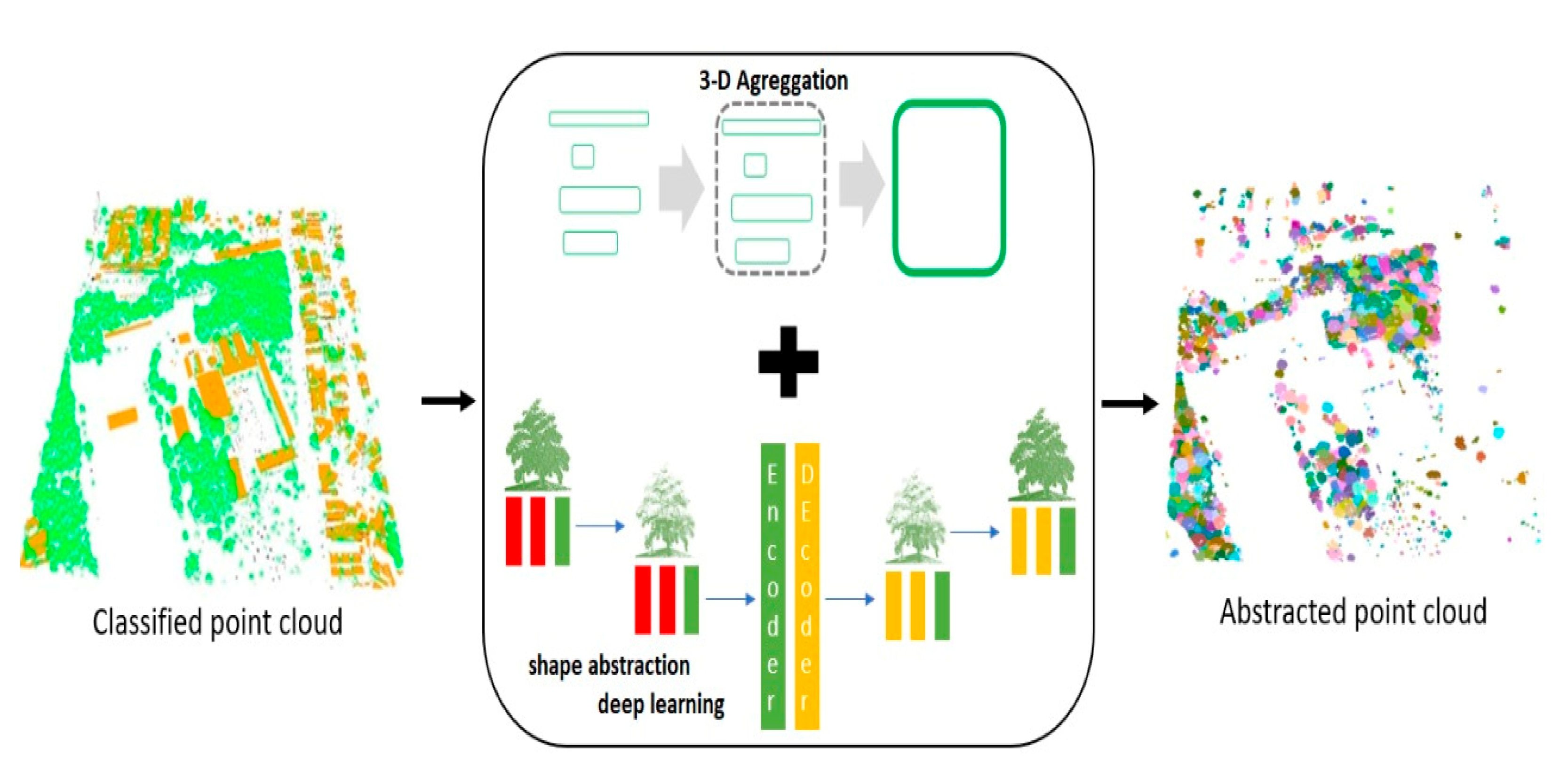
Figure 2.
The framework of the proposed method.
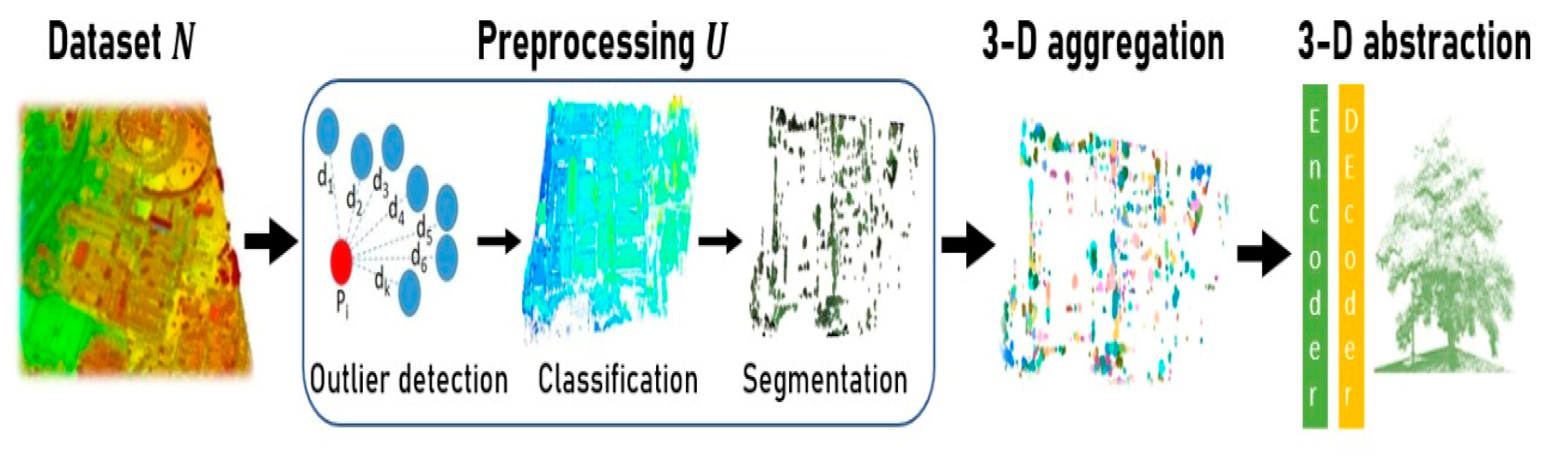
Figure 3.
Filtering of the LiDAR data: (a) Original ALS data; (b) Filtered ALS data with outliers removed; (c) Original ULS data; (d) Filtered ULS data with outliers removed.
Figure 3.
Filtering of the LiDAR data: (a) Original ALS data; (b) Filtered ALS data with outliers removed; (c) Original ULS data; (d) Filtered ULS data with outliers removed.
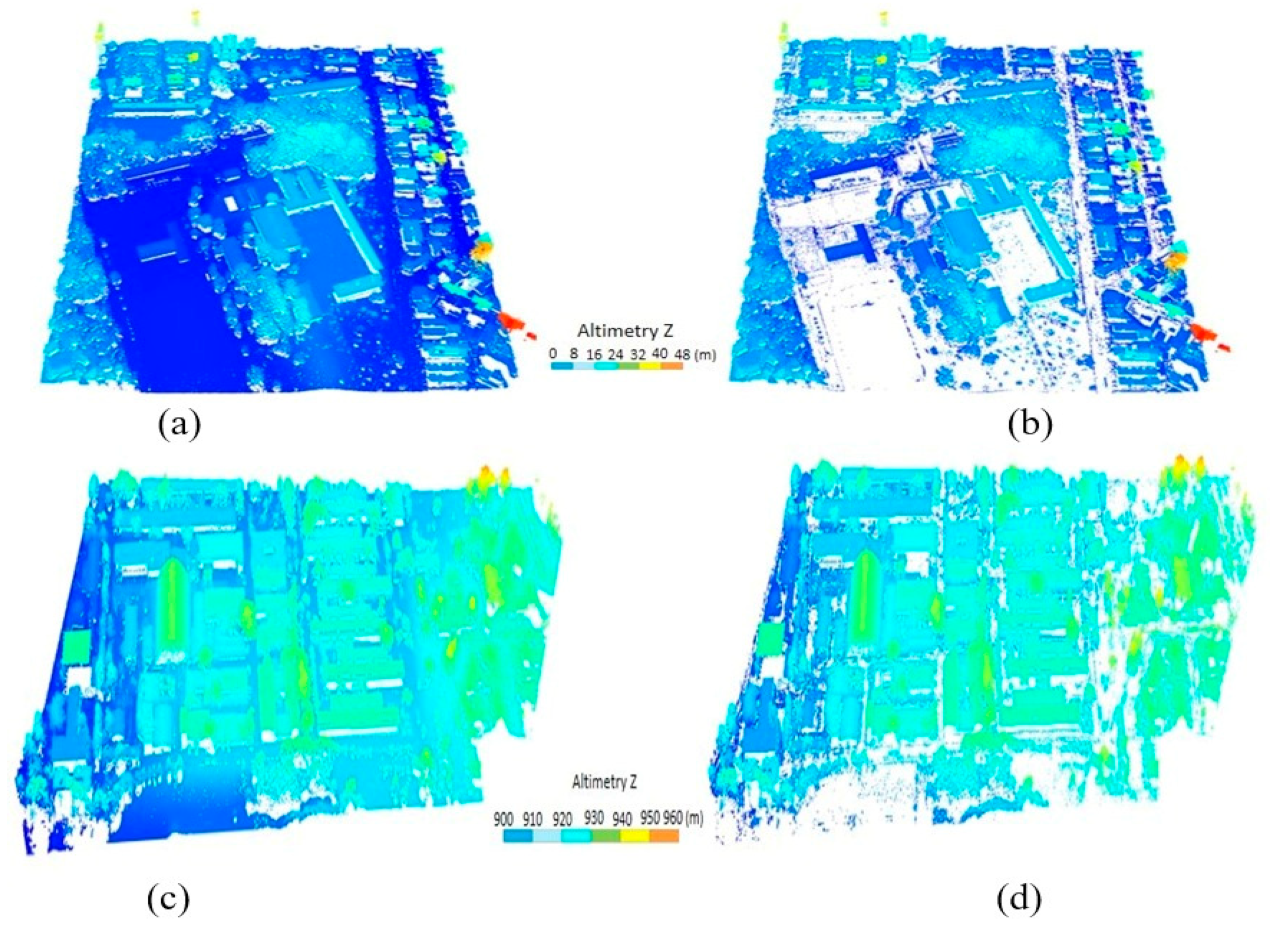
Figure 4.
Results of the initial classification: (a) Filtered ALS data; (b) Results of the initial classification of ALS data; (c) Filtered ULS data; (d) Results of the initial classification of ULS data.
Figure 4.
Results of the initial classification: (a) Filtered ALS data; (b) Results of the initial classification of ALS data; (c) Filtered ULS data; (d) Results of the initial classification of ULS data.
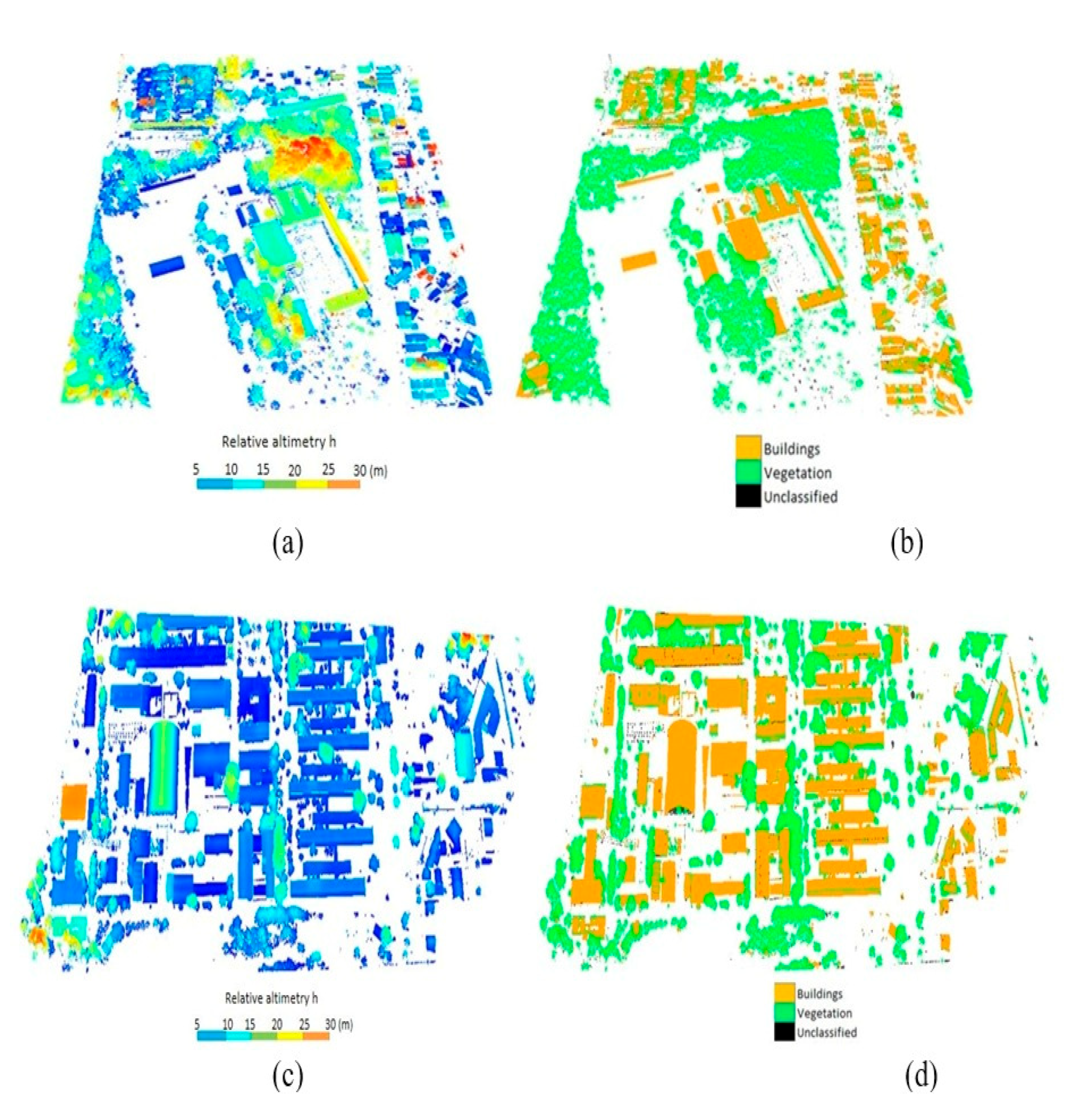
Figure 5.
Labeled vegetation points: (a) Initial classification of ALS data; (b) Results of the refined classification of ALS data; (c) Initial classification of ULS data; (d) Results of the refined classification of ULS data.
Figure 5.
Labeled vegetation points: (a) Initial classification of ALS data; (b) Results of the refined classification of ALS data; (c) Initial classification of ULS data; (d) Results of the refined classification of ULS data.
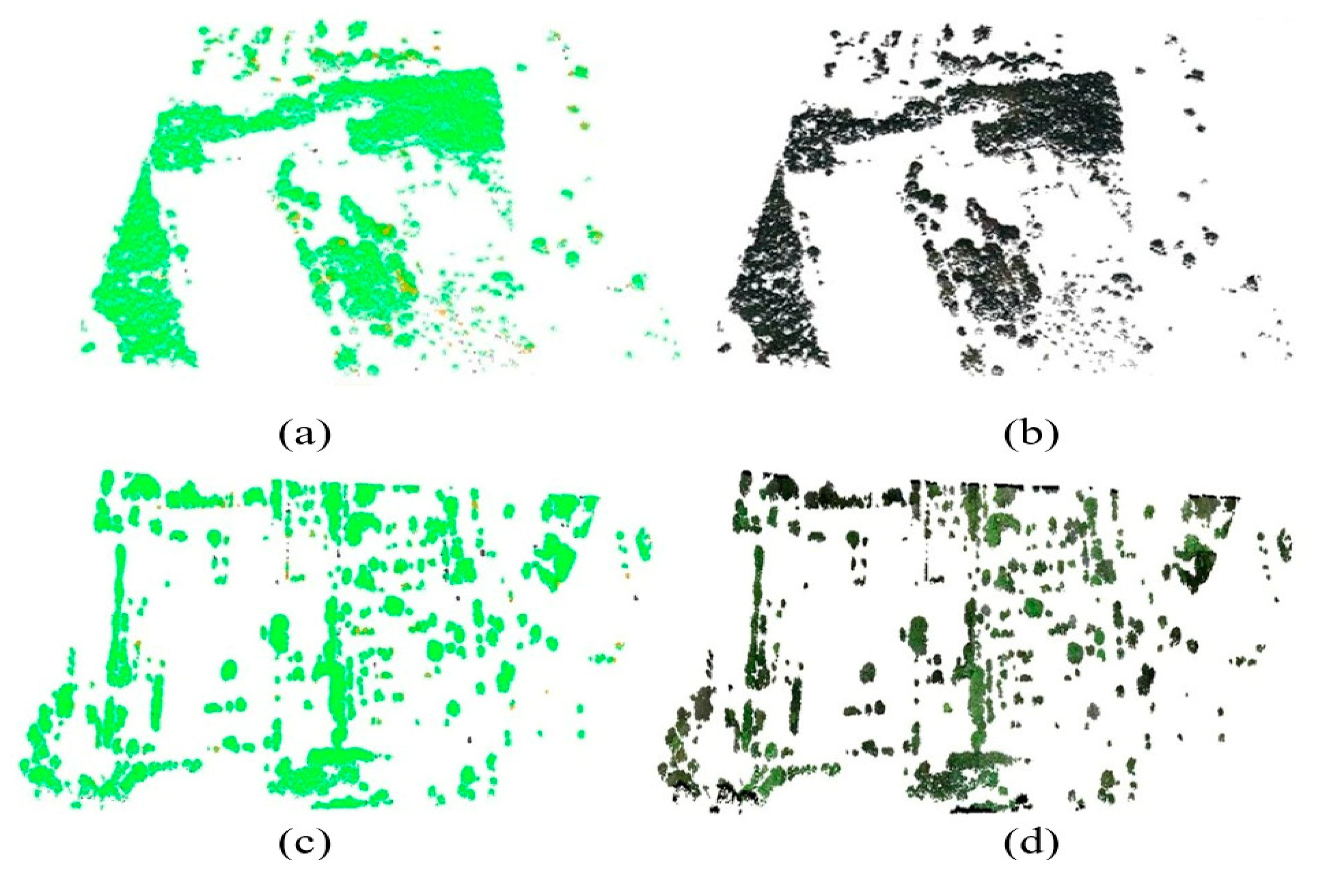
Figure 6.
Segmented individual trees: (a) Results of the segmentation of ALS data; (b) Results of the segmentation of ULS data.
Figure 6.
Segmented individual trees: (a) Results of the segmentation of ALS data; (b) Results of the segmentation of ULS data.
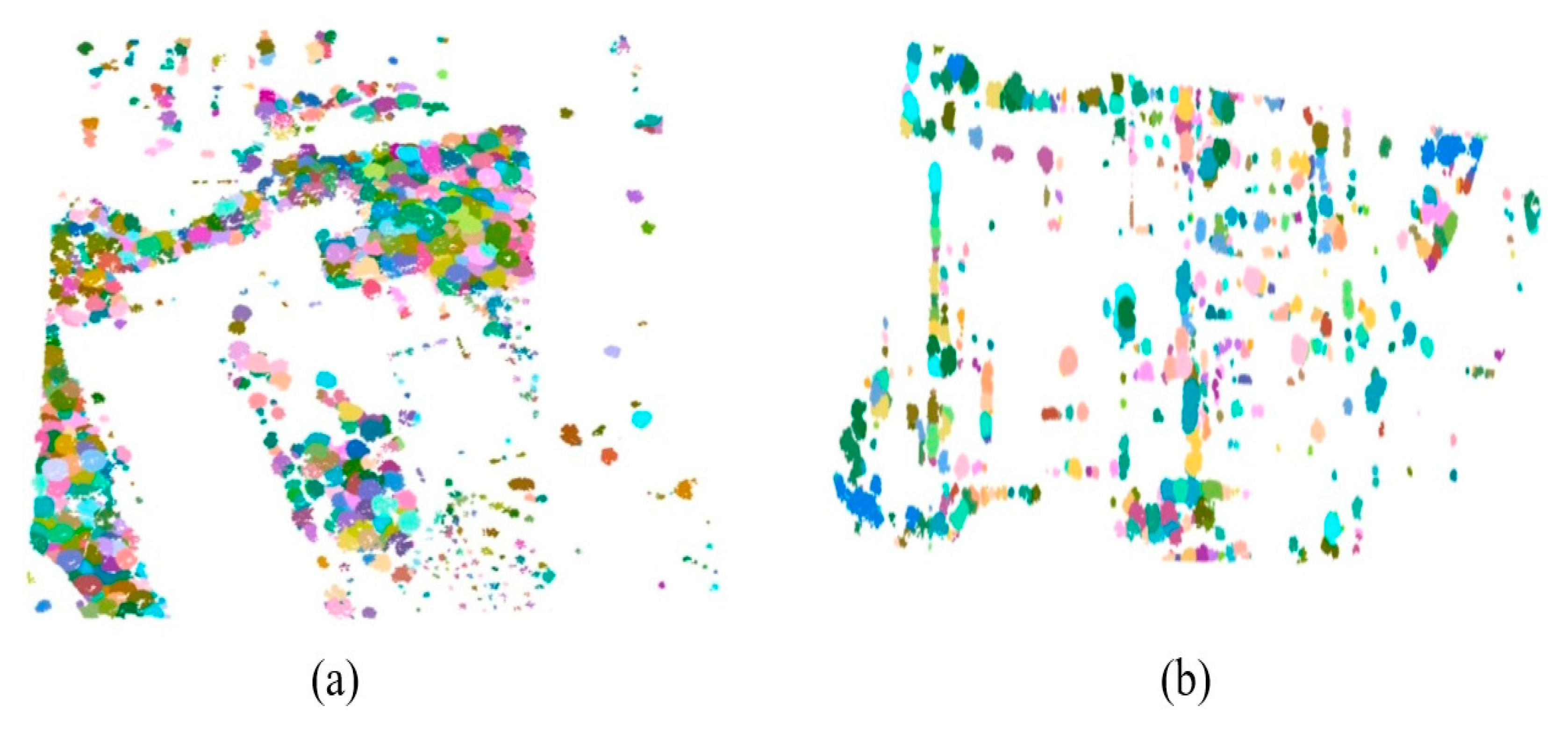
Figure 7.
Proposed 3-D aggregation threshold values.
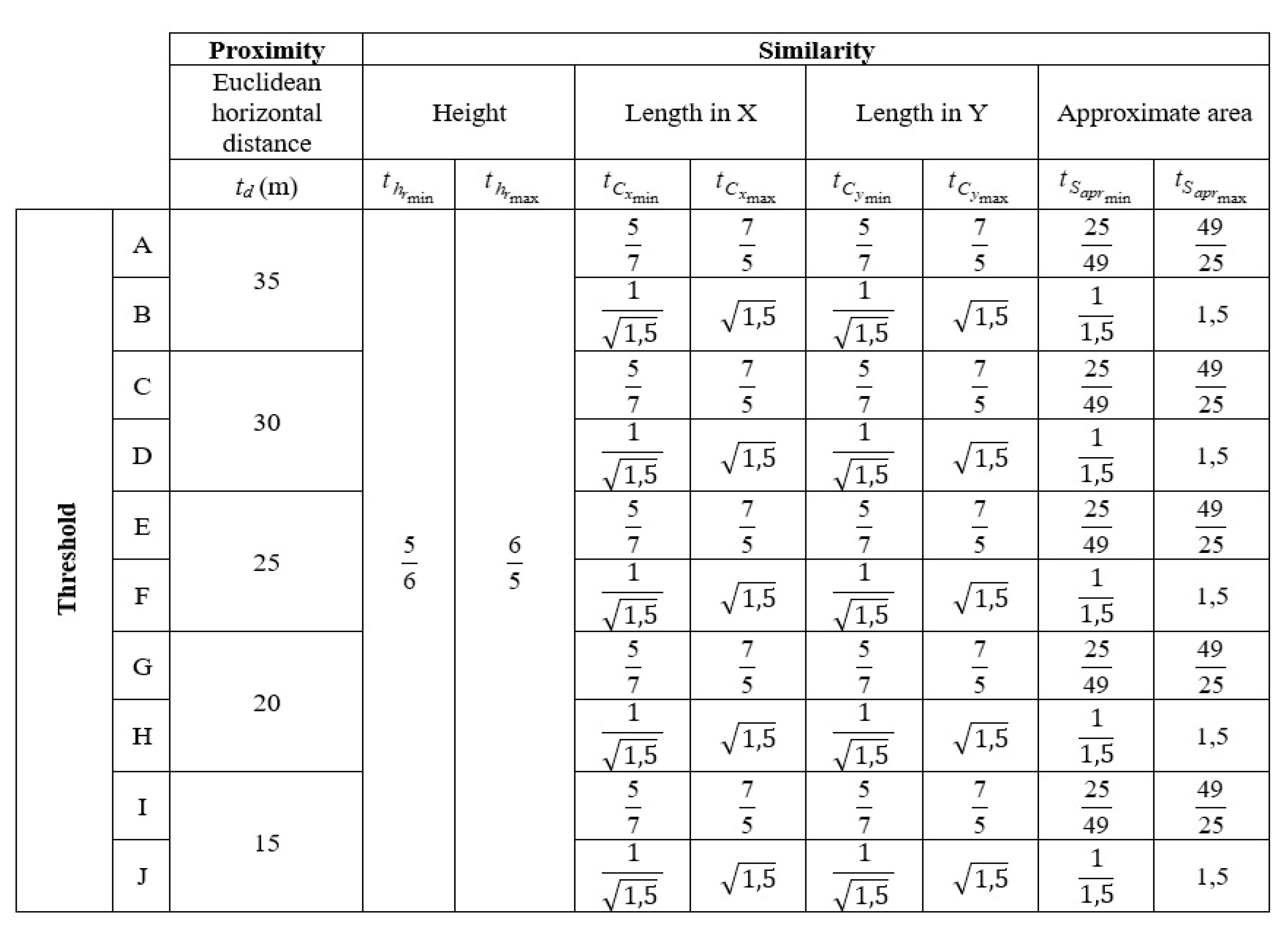
Figure 8.
3-D abstraction task: (a) Original individual tree; (b) Results of the abstraction task.
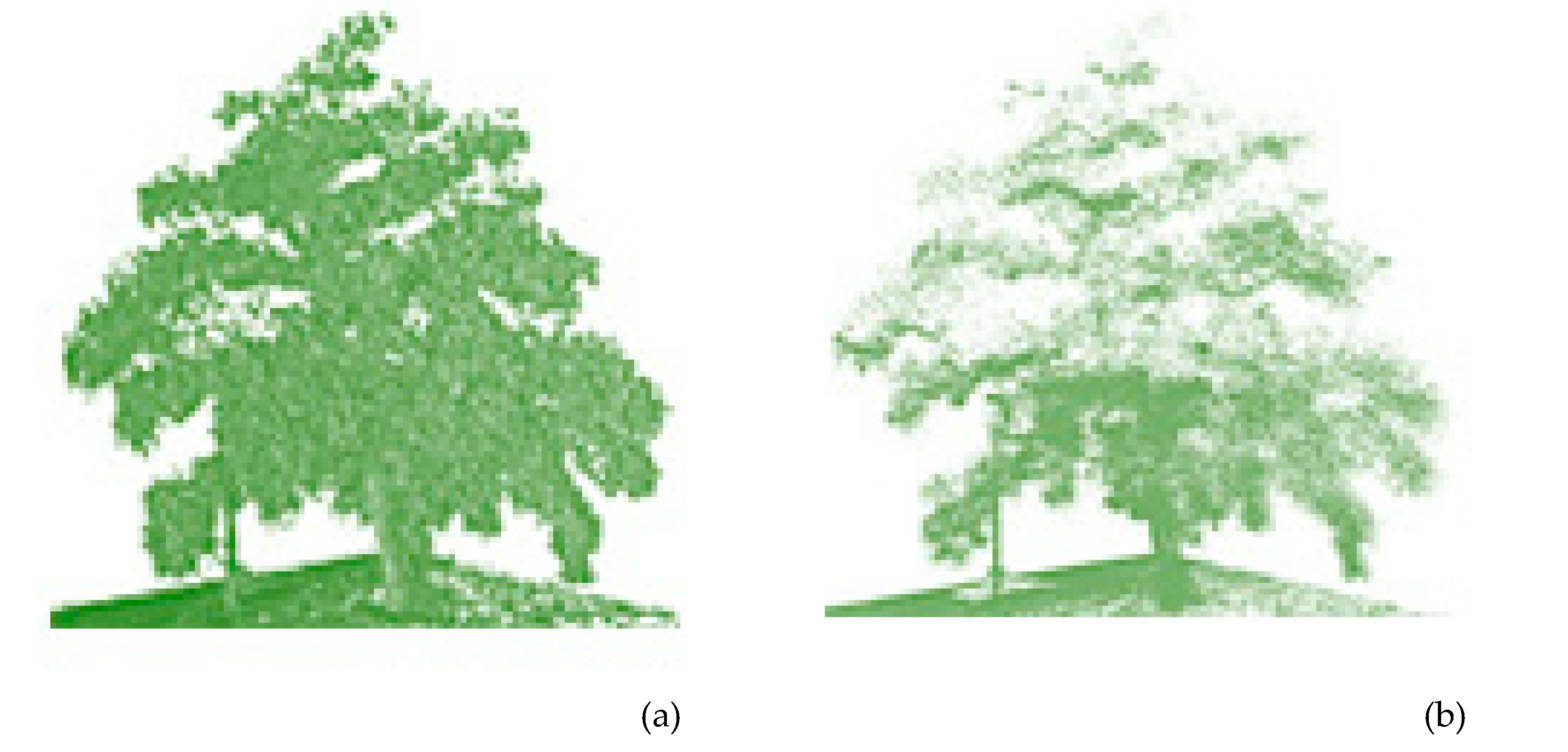
Figure 9.
Overview of reference areas: (a) Study area 1 (Salvador); (b) Orthoimage, intensity image, and Hypsometric image of the area 1; (c) Study area 2 (Curitiba); (d) Orthoimage, intensity image, and Hypsometric image of the area 2.
Figure 9.
Overview of reference areas: (a) Study area 1 (Salvador); (b) Orthoimage, intensity image, and Hypsometric image of the area 1; (c) Study area 2 (Curitiba); (d) Orthoimage, intensity image, and Hypsometric image of the area 2.
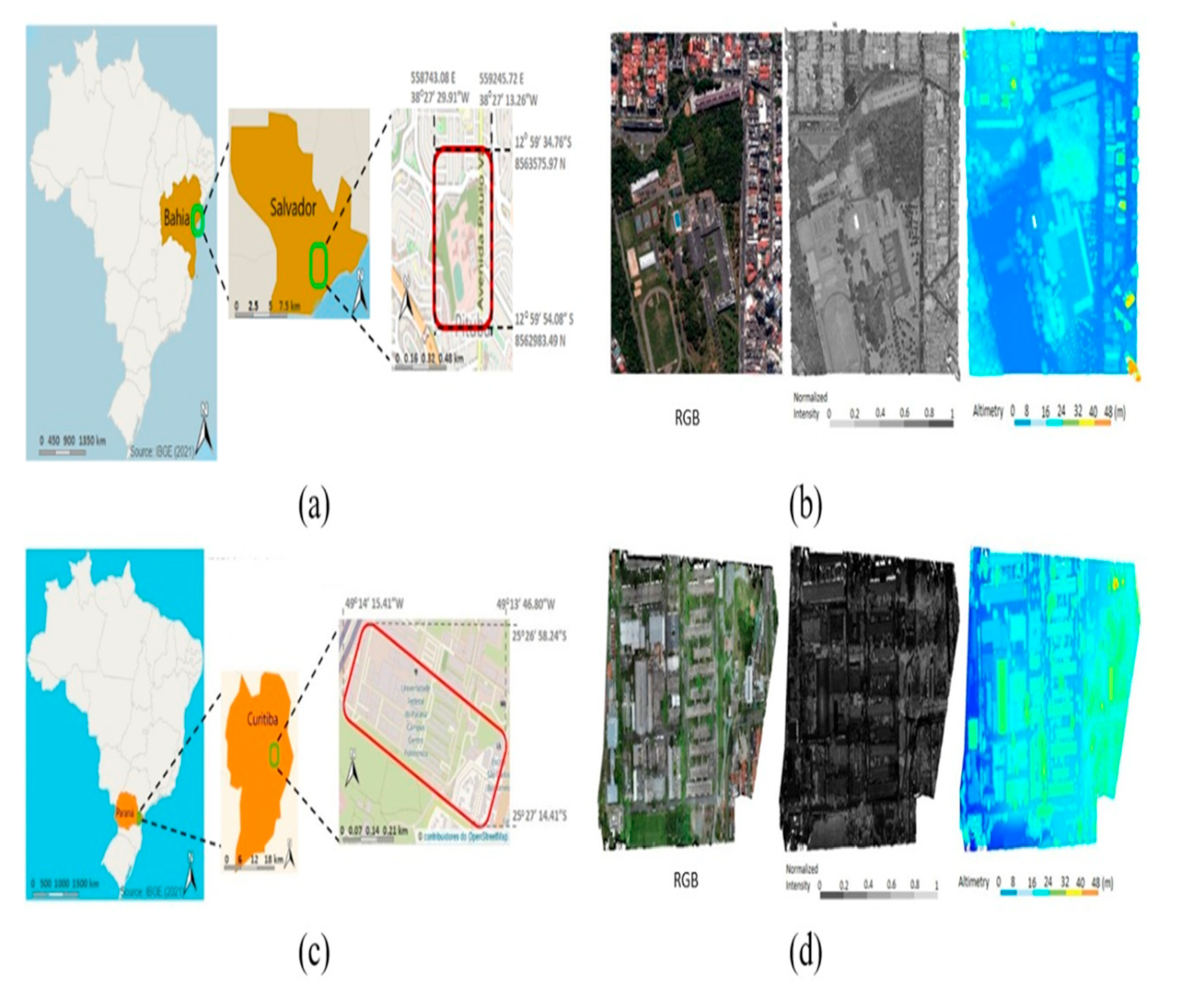
Figure 10.
3-D Aggregation results for the ALS and the ULS data after the 3-D aggregation procedure.
Figure 10.
3-D Aggregation results for the ALS and the ULS data after the 3-D aggregation procedure.
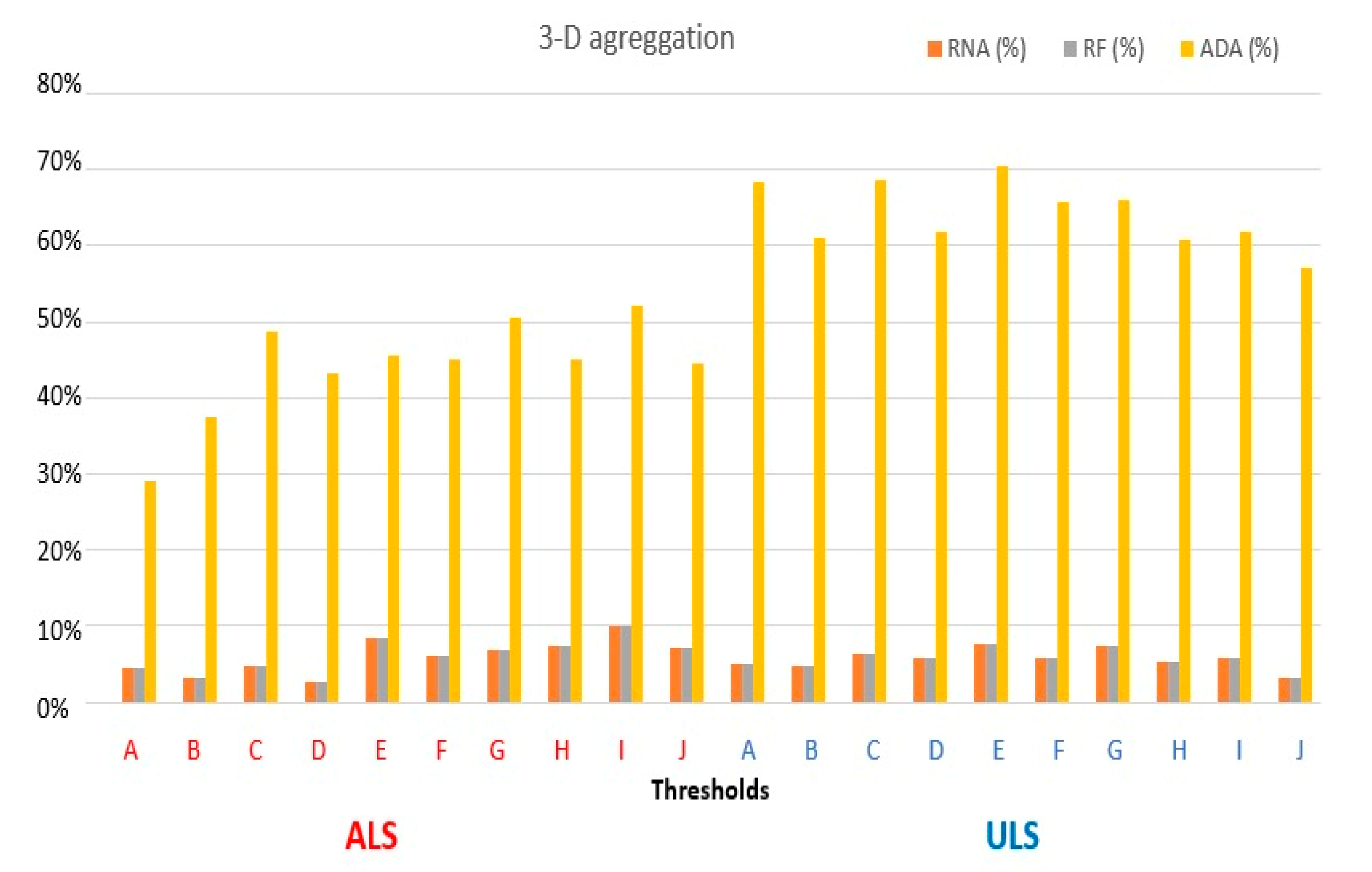
Figure 11.
Correspondence of the abstracted individual trees with the original point clouds: (a) Average horizontal displacement of centroids; (b) Average relative height variation; (c) Average crown surface area variation.
Figure 11.
Correspondence of the abstracted individual trees with the original point clouds: (a) Average horizontal displacement of centroids; (b) Average relative height variation; (c) Average crown surface area variation.
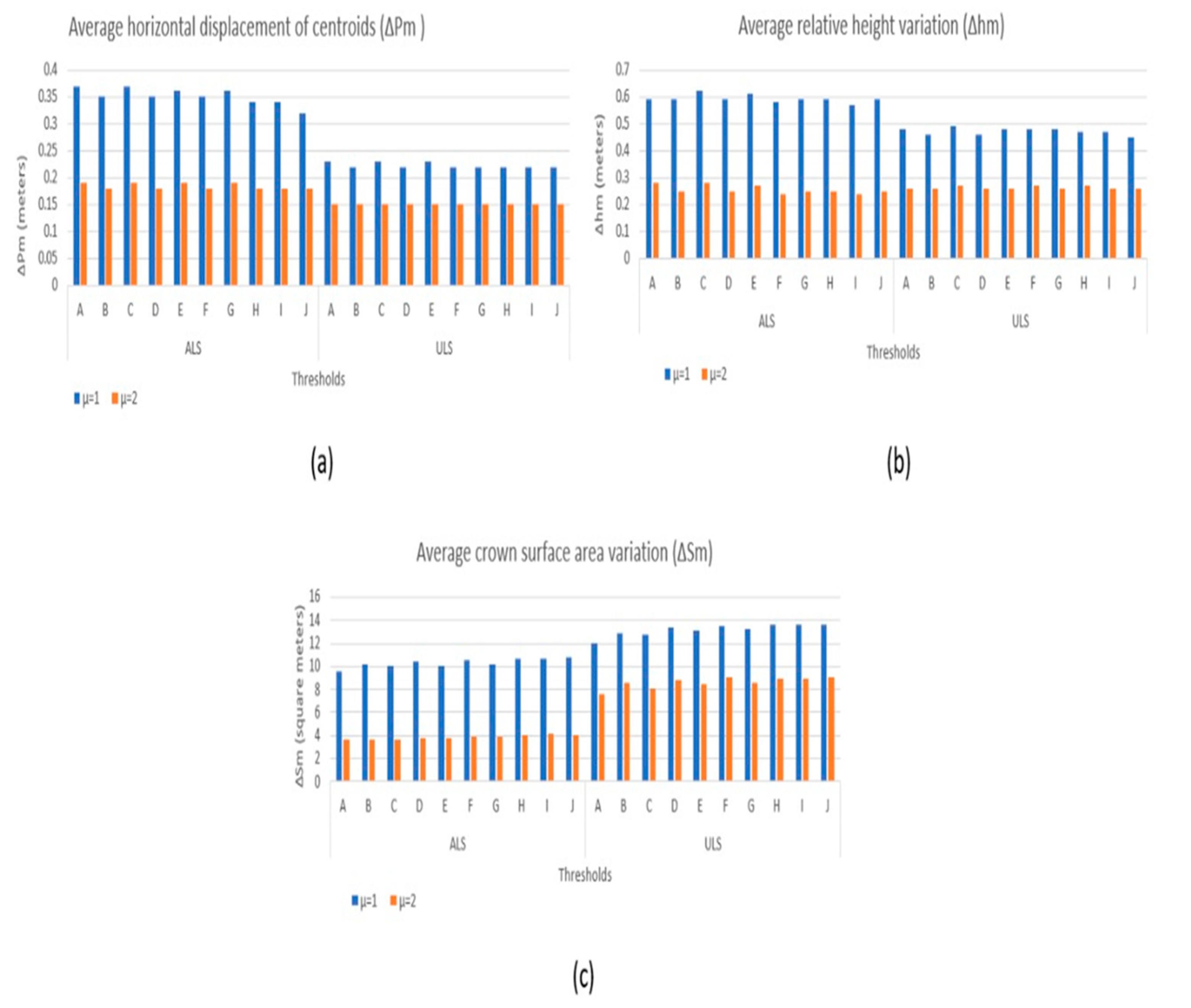

Table 1.
The spectral and local maximum criterion to analyze a labeled point Xi.
| Label | RGB criteria | Local max. criterion |
| Vegetation | XiG  2b-1; XiG > XiR; XiG > XiB 2b-1; XiG > XiR; XiG > XiB
|
Xi is local max. |
| XiG < 2b-1; XiG > XiR; XiG > XiB XiR < 2b-1; XiR < XiG; XiR XiB | ||
XiR  2b-1; XiR < XiG; XiR XiB 2b-1; XiR < XiG; XiR XiB
| ||
| Buildings | XiR  2b-1; XiR > XiG; XiR > XiB 2b-1; XiR > XiG; XiR > XiB
|
Xi is not local max. |
| XiR < 2b-1; XiR > XiG; XiR > XiB XiG  2b-1; XiG < XiR or XiG < XiB 2b-1; XiG < XiR or XiG < XiB
| ||
| XiG < 2b-1; XiG < XiR or XiG < XiB |
Table 2.
Summary of the parameters definited for tree crown segmentation (ALS and ULS data).
| Parameter | Description | Values (m) |
|---|---|---|
| dt1 | bottom limits | 5 |
| dt2 | upper limits | 7 |
| Zu | bottom limits | 15 |
| Speed up | upper limits | 10 |
| hmin | Minimum height for a detected tree | 5 |
| R | Search radius for the local maximum | 5 |
Table 3.
Confusion matrix of the point cloud classification.
| ALS | Truth reference | |||
|---|---|---|---|---|
| Vegetation | Non-vegetation | Total of points | ||
| Label | Vegetation | 500.164 | 94.225 | 594.389 |
| Non-vegetation | 18.569 | 408.114 | 426.683 | |
| Total | 518.733 | 502.339 | 1.021.072 | |
| ULS | ||||
| Label | Vegetation | 6.455.452 | 1.089.707 | 7.454.159 |
| Non-vegetation | 169.953 | 14.944.094 | 15.114.047 | |
| Total | 6.625.405 | 16.083.801 | 22.659.206 | |
Table 4.
Landscape metrics obtained with our segmentation method.
| Data | AD | DA (tree/hectare) | GF (tree/green area) | GD (m) |
|---|---|---|---|---|
| ALS | 851 | 28.65 | 67.33 | 9.73 |
| ULS | 518 | 19.9 | 78.96 | 10.45 |
Table 5.
Metrics for ALS and ULS data.
| Data | Threshold | GF(*) | GD (m) | ANA | AM |
|---|---|---|---|---|---|
| ALS | A | 64.31 | 12.56 | 431 | 382 |
| B | 65.26 | 13.37 | 554 | 271 | |
| C | 64.16 | 14.48 | 457 | 354 | |
| D | 65.58 | 13.94 | 580 | 249 | |
| E | 61.70 | 14.17 | 496 | 284 | |
| F | 63.29 | 14.11 | 625 | 175 | |
| G | 62.65 | 14.64 | 552 | 240 | |
| H | 62.34 | 14.12 | 670 | 118 | |
| I | 60.68 | 14.81 | 625 | 142 | |
| J | 62.57 | 14.07 | 722 | 69 | |
| ULS | A | 75.31 | 17.58 | 311 | 181 |
| B | 75.3 | 16.84 | 397 | 97 | |
| C | 73.93 | 17.63 | 341 | 144 | |
| D | 74.39 | 16 | 409 | 79 | |
| E | 72.68 | 17.81 | 373 | 105 | |
| F | 74.39 | 17.31 | 430 | 58 | |
| G | 73.17 | 17.35 | 405 | 75 | |
| H | 74.84 | 16.79 | 449 | 42 | |
| I | 74.39 | 16.91 | 446 | 42 | |
| J | 76.52 | 16.41 | 482 | 20 |
∗ GF in tree/square meter of green area.
Table 6.
3-D abstraction results for ALS and ULS data.
| Data | Storage space (%) | |
| µ = 1 | µ = 2 | |
| ALS | 72.65 | 45.32 |
| ULS | 98.47 | 96.94 |
Disclaimer/Publisher’s Note: The statements, opinions and data contained in all publications are solely those of the individual author(s) and contributor(s) and not of MDPI and/or the editor(s). MDPI and/or the editor(s) disclaim responsibility for any injury to people or property resulting from any ideas, methods, instructions or products referred to in the content. |
© 2024 by the authors. Licensee MDPI, Basel, Switzerland. This article is an open access article distributed under the terms and conditions of the Creative Commons Attribution (CC BY) license (http://creativecommons.org/licenses/by/4.0/).
Copyright: This open access article is published under a Creative Commons CC BY 4.0 license, which permit the free download, distribution, and reuse, provided that the author and preprint are cited in any reuse.


