Preprint
Article

Multi-objective Optimization of Energy-Efficient Multi-stage, Multi-level Assembly Job Shop Scheduling

Altmetrics

Downloads

58

Views

23

Comments

0

A peer-reviewed article of this preprint also exists.

Submitted:

02 September 2024

Posted:

03 September 2024

You are already at the latest version

Alerts
Abstract
The multi-stage, multi-level assembly job shop scheduling problem (MsMlAJSP) is commonly encountered in the manufacturing of complex customized products. Ensuring production efficiency while effectively improving energy utilization is a key focus in the industry. For the energy-efficient MsMlAJSP (EEMsMlAJSP), an improved imperialist competitive algorithm based on Q-learning (IICA-QL) is proposed to minimize the maximum completion time and total energy consumption. In IICA-QL, a decoding strategy with energy-efficient triggers based on problem characteristics is designed to ensure solution quality while effectively enhancing search efficiency. Additionally, an assimilation operation with operator parameter self-adaptation based on Q-learning is devised to overcome the challenge of balancing exploration and exploitation with fixed parameters, thus the convergence and diversity of the algorithmic search is enhanced. Finally, the effectiveness of the energy-efficient strategy decoding trigger mechanism and the operator parameter self-adaptation operation based on Q-learning is demonstrated through experimental results, and the effectiveness of IICA-QL for solving EEMsMlAJSP is verified by comparing with other algorithms.
Keywords: 
Subject: Engineering  -   Control and Systems Engineering

1. Introduction

Since the manufacturing industry is one of the most energy-intensive sectors, how to effectively improve energy efficiency while maintaining production efficiency is currently a major focus within the industry. Energy-efficient scheduling (EES) utilizes limited resources to rationally arrange production and optimize the production process, which is an effective way to effectively reduce the energy consumption in manufacturing systems. Recently, EES has been successfully applied to various scheduling problems in discrete manufacturing industries, yielding positive results.
As an extension of the classic job shop scheduling problem (JSP), the multi-stage, multi-level assembly job shop scheduling problem (MsMlAJSP), which not only involves multiple stages of production from processing to assembly, but also considers complex assemblies composed of multiple jobs with a tree-like multi-level structure consisting of components and subassemblies. It plays an important role in quickly responding to the manufacturing of customized products with multi-variety and small batch. Wang et al. [1] addressed the distributed MsMlAJSP considering maintenance, aiming to minimize the maximum tardiness. Cheng et al. [2] proposed batch transfer and mixed-model assembly for MsMlAJSP with the optimization objectives of minimizing manufacturing and transportation costs. Building on this, Cheng et al. [3] further considered lot streaming with the objective of minimizing total completion time and production cost. All of the above studies have already conducted relevant work on MsMlAJSP, primarily focusing on improving production efficiency and economic benefits. However, as the number of product structural levels and manufacturing stages increases, constraints become more complex, leading to idle time between and within stages, which results in significant idle energy consumption. Therefore, further research is needed on the energy-efficient multi-stage, multi-level assembly job shop scheduling problem (EEMsMlAJSP) for complex multi-level products.
The EEMsMlAJSP is highly complex with a vast solution space, presenting challenges for efficient resolution. Currently, solving the energy-efficient scheduling problem in complex manufacturing systems mainly focuses on energy-efficient strategies and algorithm design. Among these, the block-moving energy-efficient strategy, which makes operations within stages more compact by moving process operations, can effectively reduce idle energy consumption. This is currently an effective method for handling multi-operation and multi-stage complex scheduling problems [4,5,6,7]. There are two main approaches: one is to apply the block-moving strategy only to the solutions in the non-dominated set to further reduce energy consumption [8]; however, this operation may cause the loss of some potential solutions, resulting in a local rather than a global optimum. The other approach is to embed the block-moving strategy into the individual decoding process to avoid losing the global optimal solution [9]; however, such design can lead to a waste of computational resources and severely slow down the search efficiency of algorithm. Therefore, it is an urgent need to design an efficient block-moving strategy that improves solution quality and search efficiency without losing the global optimum.
In terms of algorithm design, the imperialist competitive algorithm (ICA) is an effective evolutionary algorithm framework. It facilitates population evolution through mechanisms such as the assimilation, colonial revolutions, and imperial competition, demonstrating efficient global and local search capabilities. For the past few years, ICA has been successfully applied to solving various multi-objective energy-efficient scheduling problems, such as multi-objective energy-efficient flexible job shop scheduling with energy consumption thresholds [10], energy-efficient hybrid flow shop scheduling [11], energy-efficient flexible job shop scheduling considering transportation and setup times [12], and energy-efficient flexible job shop batch scheduling [13]. For the assimilation in the global search of the algorithm, existing studies mostly adopt the Uniform Crossover (UX) operator, with the probability parameters of uniform crossover preset through experiments. However, applying traditional static parameters to ICA may not ensure optimal search efficiency and solution quality due to the complexity of the EEMsMlAJSP problem. Therefore, it is necessary to design a reasonable dynamic parameter adaptive adjustment mechanism to balance the exploration and exploitation of the algorithm. Reinforcement Learning (RL), such as Q-learning, offers strong decision-making and optimization capabilities. Recent studies have shown that Q-learning can effectively adjust algorithm parameters, enhancing the balance between exploration and exploitation and improving solution quality [14,15,16].
In summary, we propose an improved ICA based on Q-learning (IICA-QL) to solve the EEMsMlAJSP, aiming to the maximum completion time and total energy consumption. First, a mathematical model of the problem is established, and an energy-efficient strategy decoding trigger mechanism is designed to simultaneously enhance solution quality and search efficiency. Second, the IICA-QL for solving the EEMsMlAJSP is proposed. In IICA-QL, two heuristic rules and a random generation method are used to collaboratively construct an initial population with high quality and diversity. A dynamic adaptive adjustment strategy for assimilation operator parameter is implemented based on Q-learning to enhance convergence speed while maintaining population diversity, thus the exploration and exploitation capabilities of the algorithm are better balanced. A hyper-heuristic variable neighborhood search-guided revolution operation is designed to conduct detailed searches on identified high-quality colonies. The competitive phase is replaced with a joint imperialist invasion operation to achieve cooperative co-evolution and information exchange among multiple empires, resulting in more evenly distributed non-dominated solutions. Finally, the effectiveness of the proposed algorithm in solving the EEMsMlAJSP is verified through experimental results and comparison with other algorithms.
The specific structure of the paper is as follows: The problem definition and Mathematical model are established in Section 2. The encoding and decoding design is presented in Section 3. The introduction of the improved imperialist competitive algorithm based on Q-learning (IICA-QL) is described in Section 4. Experimental results and analysis are provided in Section 5. The conclusion to the paper is given in Section 6.

2. Problem Formulation

Table 1. Notations of mathematical model.
Notations Descriptions
Indices
z Index of products, z = 1 , 2 , , N P
j Index of jobs, j = 1 , 2 , , N Q
i Index of processing operations, i = 1 , 2 , , N O
a Index of assembly operations, a = 1 , 2 , , N A
m Index of processing machines, m = 1 , 2 , , N M
t Index of transportation vehicles, t = 1 , 2 , , N T
w Index of transportation vehicle load transportation, w = 1 , 2 , , N t w
k Index of assembly machines, k = 1 , 2 , , N K
Parameters
M The set of processing machines, M = { M 1 , , M m , , M N M }
V The set of transportation vehicles, V = { V 1 , , V t , , V N T }
K The set of assembly machine, K = { K 1 , , K k , , K N K }
P The set of products, P = { P 1 , , P z , , P N P }
N p Number of products
N Q Number of jobs
N O Number of processing operations
N A Number of assembly operations
N M Number of processing machines
N T Number of transportation vehicles
N K Number of assembly machines
N O m , N A k Number of operations on processing machine m and assembly machine k
N t w Number of load transportations by vehicle t
G m a x Maximum load capacity of the vehicle
J j , J z The job indexed by j, the set of all jobs belonging to P z
O j i , O j The i-th processing operation of J j , the set of all operations of J j
A z a , A z The a-th assembly operation and the set of assembly operations of P z
M j i The set of machines available for processing operation O j i
P P m , P P k Unit power consumption of processing machine m and assembly machine k in working mode
P I m , P I k Unit power consumption of processing machine m and assembly machine k in standby mode
P S m Unit power consumption of processing machine m in setup mode
P T t Unit power consumption of transportation vehicle t
D i s P A Distance between the processing shop and the assembly shop
V 0 , V t w Speed of transportation vehicles when unloaded and speed of transportation vehicle t during the w-th load transportation
P ( π i m ) , P ( π a k ) Processing time of operation π i m and π a k
S P ( π i 1 m , π i m ) Setup time of operation π i 1 m and π i m
I P ( π i 1 m , π i m ) Idle time between operation π i 1 m and π i m excluding setup time
I P ( π a 1 k , π a k ) Idle time between operation π a 1 m and π a m
R T ( π 1 m ) Release time of job π 1 m
Decision variables
π m = [ π 1 m , π 2 m , , π N O m m ] Sequence of operations on processing machine m
π k = [ π 1 k , π 2 k , , π N A k k ] Sequence of operations on assembly machine k
π s t 1 , π s t 2 , π s t 3 Sequence of operations on processing stage, transportation stage, and assembly stage
S T ( π a k ) , C T ( π a k ) Start time and completion time of operation π a k
E C R s t 1 , E C S s t 1 , E C P s t 1 , E C I s t 1 Release energy consumption, setup energy consumption, processing energy consumption, and idle energy consumption in the processing stage
E C A s t 3 , E C I s t 3 assembly energy consumption and idle energy consumption in the assembly stage
E C s t 1 , E C s t 2 , E C s t 3 Energy consumption in the processing stage, transportation stage, and assembly stage
C max Maximum completion time of a schedule
TEC Total energy consumption

2.1. Problem Definition

The EEMsMlAJSP addressed in this work consists of multiple stages, including processing, transportation, and assembly. The problem is defined as follows. In the processing stage, transportation stage, and assembly stage, there are N M flexible processing machines M = { M 1 , , M m , , M N M } , N T transportation vehicles V = { V 1 , , V t , , V N T } with the same load capacity G m a x , and N K assembly machines K = { K 1 , , K k , , K N K } , respectively. There is a product set P = { P 1 , , P z , , P N P } that needs to be manufactured, where each product P z P is composed of a set of various jobs J z and should undergo an assembly operation set A z to be assembled into the final product. Each job J j J z has a release time and consists of a set of processing operations O j . all operations O j i O j must be completed before the J j can be transported in batches by vehicles with load capacity constraint. Once all jobs J j ​ belonging to a product P z have been transported to the assembly stage, the assembly of P z can begin. In the processing stage, each operation O j i has a set of compatible machines M j i from which one machine is selected for processing. Once the operation is completed, the next operation for job J j processed according to the specified sequence. In the transportation stage, a fleet of vehicles V is available to transport jobs from the processing stage to the assembly stage. Each vehicle V t V departs from the processing shop and must return after completing its transportation tasks. The vehicles are subject to capacity constraints and are allowed to make multiple trips, with each trip carrying a batch of components produced in the processing stage. In the assembly stage, once all components belonging to product P z ​ are ready, all operations​ A z a A z are sequentially completed according to the assembly process.
The optimization objectives of this problem are to simultaneously minimize C max and TEC. It is a multi-objective problem and encompasses several sub-problems, including the sequencing of processing operations, assignment of processing machines, sequencing of job transportation, assignment of vehicles, sequencing of product assembly, sequencing of assembly operations and assignment of assembly machines. The computational complexity of the mathematical model is O = ( ( N O ! ) × N M N O × ( N Q ! ) × N T N Q × ( N P ! ) × N K N A ) . So as the problem size increases, the complexity grows exponentially. Moreover, as an extension of the well-known NP-hard problem JSP, the EEMsMlAJSP integrates assembly and batch transportation, making it an NP-hard problem as well, and even more complex.
The schematic diagram of the EEMsMlAJSP model is shown in Figure 1. Some assumptions are listed below:
  • In the processing and assembly stages, any machine can only process one operation at a time.
  • Once started, processing operations, transportation processes, and assembly operations cannot be interrupted.
  • All machines and vehicles are available at time zero.
  • Transportation time between machines for consecutive processing (or assembly) operations is not considered.
  • Vehicles maintain a constant speed during transportation.
  • The initial setup time is included in the release time of the workpiece.

2.2. Mathematical Model

The mathematical model for the three stages with two optimization objectives in EEMsMlAJSP is constructed as follows:
The first objective, the maximum completion time, is the time when all products are fully assembled, calculated as follows:
C max = max { C T ( π a k ) } , a , k
The second objective, namely total energy consumption, is composed of three parts: total energy consumption in the processing stage, total energy consumption in the transportation stage, and total energy consumption in the assembly stage. The total energy consumption for each stage is calculated as follows:
(1) Processing stage: The total energy consumption in this stage is composed of the energy consumption of the processing machines, which is determined by four modes of machines: release mode, setup mode, working mode, and idle mode. The energy consumption for each mode of the processing machines is constructed as follows:
Release energy consumption: This refers to the energy consumption of machines before the first arrival time of the job. The release energy consumption in the processing stage is calculated as follows:
E C R s t 1 = m = 1 N M P P m × R T ( π 1 m )
Setup energy consumption: This energy consumption generated during the preparation process of the machine before entering the working mode. The setup energy consumption in the processing stage is calculated as follows:
E C S s t 1 = m = 1 N M i = 2 N O m P S m × S P ( π i 1 m , π i m )
Working energy consumption: The energy consumption generated when the processing machine is in working mode. The working energy consumption in the processing stage is calculated as follows:
E C P s t 1 = m = 1 N M i = 1 N O m P P m × P ( π i m )
Idle energy consumption: The energy consumption generated during the time between processing two consecutive operations, excluding setup time. The idle energy consumption in the processing stage is calculated as follows:
E C I s t 1 = m = 1 N M i = 2 N O m P I m × I P ( π i 1 m , π i m )
The total energy consumption in the processing stage is calculated as follows:
E C s t 1 = E C R s t 1 + E C S s t 1 + E C P s t 1 + E C I s t 1
(2) Transportation stage: The total energy consumption in this stage consists of the energy consumption of the transportation vehicles, which is composed of two parts: loaded energy consumption and unloaded energy consumption. The total energy consumption in the transportation stage is calculated as follows:
E C s t 2 = t = 1 N T w = 1 N t w P T t × ( D i s P A V 0 + D i s P A V t w )
(3) Assembly stage: The total energy consumption in this stage consists of the energy consumption of the assembly machines, which is composed of two modes of modes: working mode and idle mode. The energy consumption for each mode of the assembly machines is constructed as follows:
Working energy consumption: The energy consumption generated when the assembly machine is in working mode. The working energy consumption in the assembly stage is calculated as follows:
E C A s t 3 = k = 1 N K a = 1 N A k P P k × P ( π a k )
Idle energy consumption: This refers to the energy consumption generated between two consecutive operations on the same assembly machine. The idle energy consumption of the machine in the assembly stage is calculated as follows:
E C I s t 3 = k = 1 N K a = 2 N A k P I k × I P ( π a 1 k , π a k )
The total energy consumption in the assembly stage is calculated as follows:
E C s t 3 = E C A s t 3 + E C I s t 3
The total energy consumption of the three stages is calculated as follows:
T E C ( π ) = E C s t 1 + E C s t 2 + E C s t 3
Optimization objective: To find an optimal sequence in the set of all three-stage sequences ( π = [ π s t 1 , π s t 2 , π s t 3 ] ) that simultaneously minimizes the maximum completion time and total energy consumption. The specific details are as follows:
C max ( π ) = max { C T ( π a k ) } , a , k
T E C ( π ) = E C s t 1 + E C s t 2 + E C s t 3
{ C max ( π * ) = min { C max ( π s t 1 , π s t 2 , π s t 3 ) } , T E C ( π * ) = min { T E C ( π s t 1 , π s t 2 , π s t 3 ) } π * = arg { C max ( π s t 1 , π s t 2 , π s t 3 ) T E C ( π s t 1 , π s t 2 , π s t 3 ) } min , ( π s t 1 , π s t 2 , π s t 3 )

3. Encoding and Decoding Design

As described in Section 2.1, the problem characteristics of EEMsMlAJSP result in an exceptionally large solution space. If full encoding is applied to each stage, although the entire solution space can be effectively represented, it also results in the algorithm convergence being slowed and invalid solutions generated during the algorithm iteration process needing to be repaired, thus affecting the search efficiency of the algorithm. Heuristic rules can effectively trim the solution space while maximizing the discovery of near-optimal solutions to the problem, thereby the convergence speed of the algorithm is improved. Therefore, based on the coupling properties between the stages of EEMsMlAJSP [17,18], only the processing operations in the processing stage are encoded, with the assignment of processing machines and the sub-problems in subsequent stages being decoded using heuristic rules.

3.1. Encoding

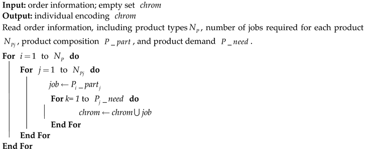
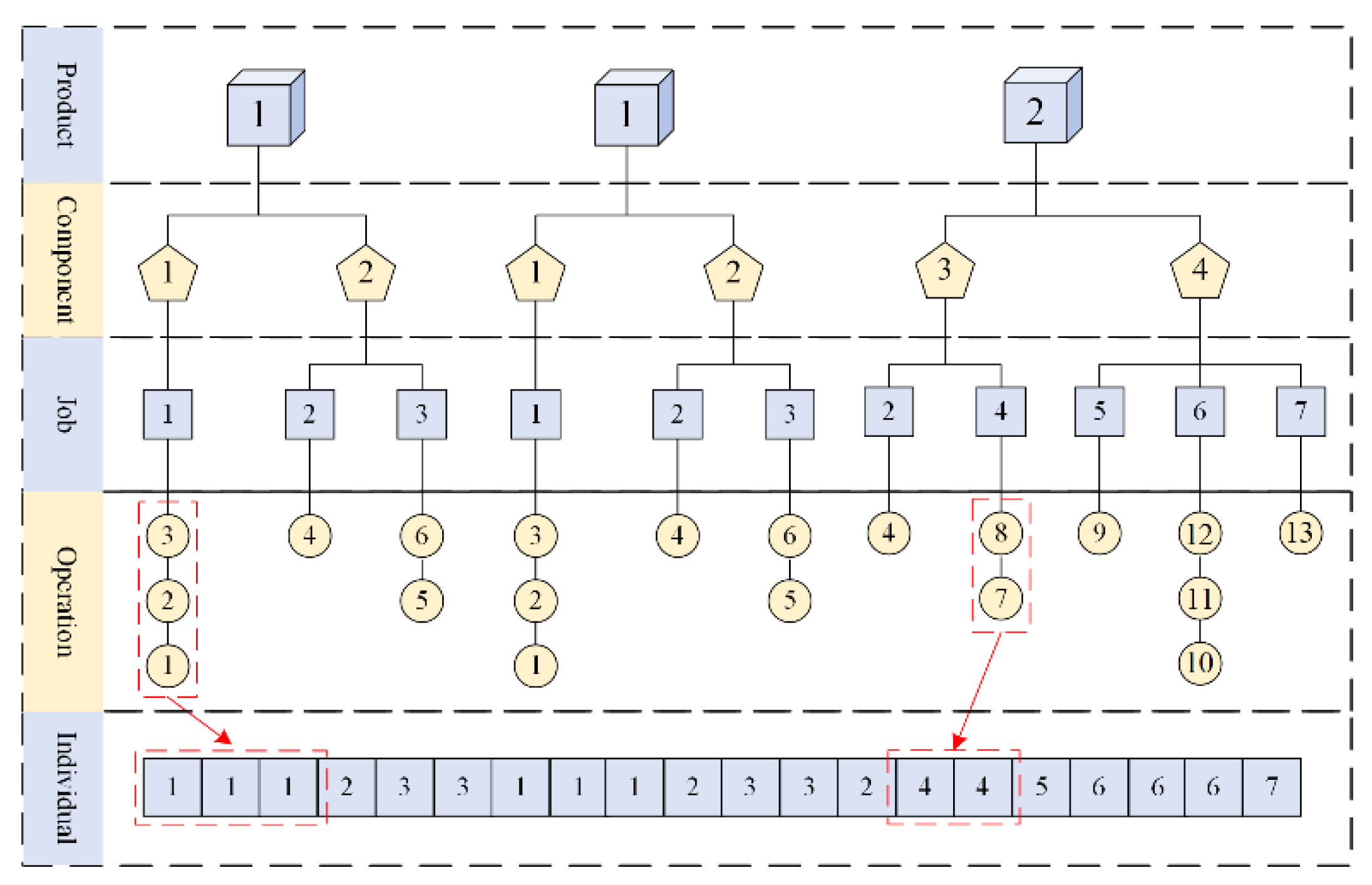
In this study, the solution to the problem is represented using an operation-based encoding method. The operations of a job are indicated by number of the job, and the number of times that the job number appears represents which operation it is for that job. Due to the design order requirements of the products considered in this paper, and the possibility of identical jobs existing among different products, product information needs to be read sequentially to determine the required jobs for the product, and each job is assigned a unique code for identification. The pseudocode for the encoding is shown in Algorithm 1.
Algorithm 1 Encoding Method
Preprints 116981 i001
To better illustrate the encoding process, we use an example where the demand for product 1 is 2 and the demand for product 2 is 1. Product 1 consists of components 1 and 2, while product 2 consists of components 3 and 4. Component 1 is composed of job 1, component 2 is composed of jobs 2 and 3, component 3 is composed of jobs 2 and 4, and component 4 is composed of jobs 5, 6 and 7. Each job is processed through corresponding operations. The specific encoding method for this example is shown in Figure 2.

3.2. Decoding Rules

To narrow the solution space while maximizing the discovery of near-optimal solutions to the problem, the heuristic decoding rules for allocation in the processing stage and subsequent transportation and assembly stages are as follows:
(1)
Machine assignment in the processing stage
The earliest completion time (ECT) rule is used to assign operations to the machine that can complete them the earliest. If multiple machines can complete the operation at the same time, the minimum energy consumption first (MECF) rule is applied to select the machine with the lowest energy consumption.
(2)
Jobs transportation sequence and vehicle allocation in the transportation stage
Under the constraint of vehicle load capacity, the first ccompleted first transported (FCFT) rule is used to organize the batch transportation of jobs. This means that jobs are loaded into available vehicles in the order of their completion times, ensuring that no single vehicle is overloaded. Subsequent jobs are transported by following vehicles according to the same rule.
(3)
Product assembly sequence and machine assignment in the assembly stage
When the jobs transported to the assembly shop are sufficient for the complete assembly of the product, the assembly is carried out according to the product assembly process. If multiple products simultaneously meet the assembly conditions, the minimum jobs first (MJF) rule is used to determine the assembly sequence. During product assembly, the machine assignment for assembly operations follows the same rules as in the processing stage to determine the assembly machine for each operation.

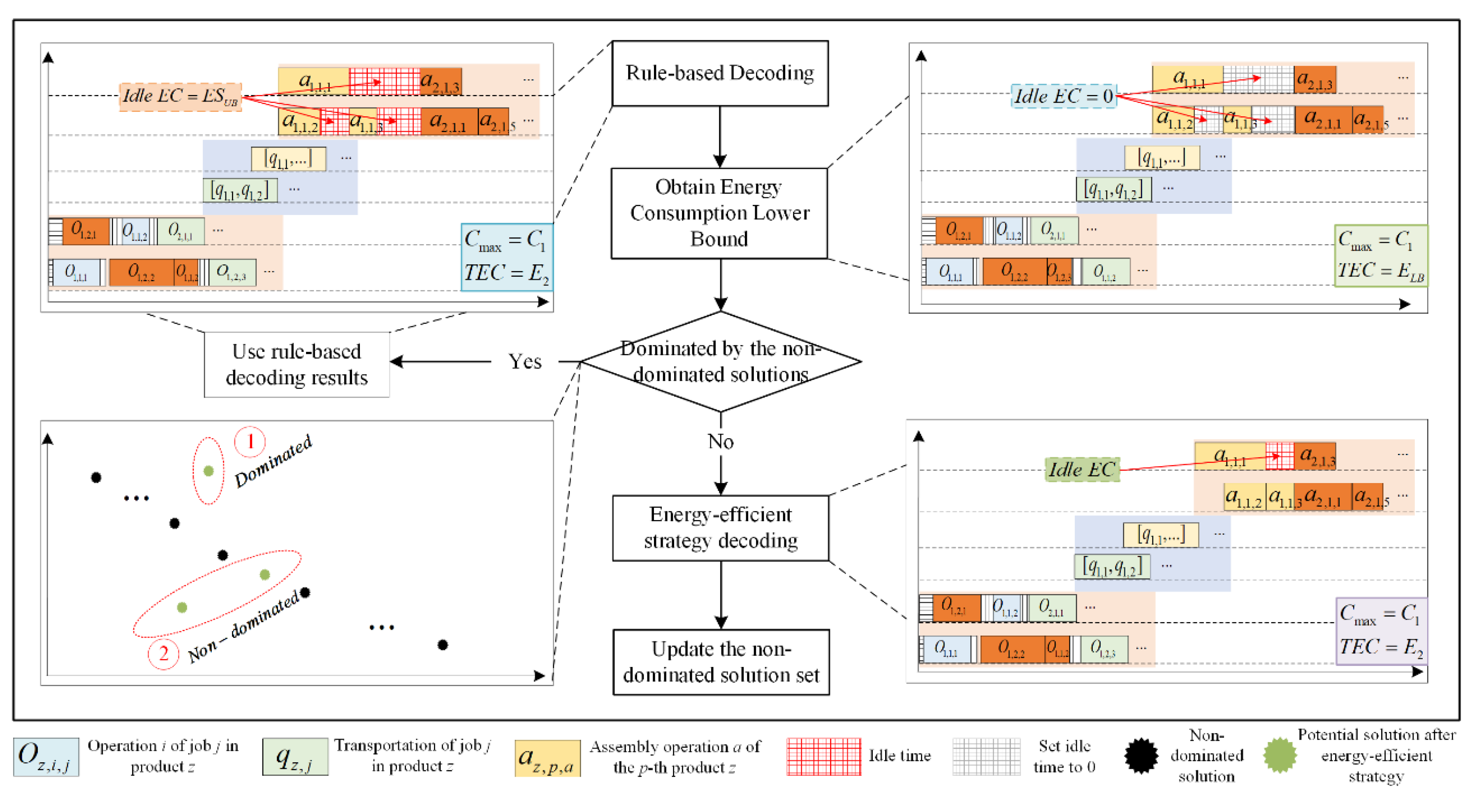
3.3. Design of Energy-Efficient Strategy Decoding Trigger Mechanism

To address the issue of substantial idle energy consumption caused by the hierarchical coupling characteristics of EEMsMlAJSP, an energy-efficient strategy based on block-moving can reduce machine idle time by making dispersed operations more compact without changing the maximum completion time, thus reducing the idle energy consumption generated by machines.
However, as the problem scale increases, executing the energy-efficient strategy usually takes a long time and consumes significant computational resources. In fact, not all solutions benefit from this strategy in terms of improving the quality of non-dominated solutions. Therefore, we propose an adaptive trigger mechanism for the energy-efficient strategy decoding, which ensures potential high-quality solutions are not lost while improving the search efficiency. The specific operations are as follows:
Step 1: Apply the decoding rules and the active decoding method [19] to the individual to obtain the scheduling results C max ( π ) and T E C ( π ) , and record the idle time of all machines.
Step 2: According to Equation (15) and Equation (16), obtain the upper bound of energy savings E S U B and the lower bound of energy consumption E L B respectively for the scheduling scheme after applying the energy-efficient strategy.
Step 3: Determine the relationship between ( C max ( π ) , E L B ) and the current non-dominated solutions. If it is not dominated by the current non-dominated solutions or if they are mutually non-dominating, proceed to Step 5, otherwise, proceed to Step 4.
Step 4: Use the objective values C max ( π ) and T E C ( π ) obtained from the decoding rules as the decoding results of the scheduling scheme.
Step 5: Following the product assembly sequence of the scheduling scheme, check each product in reverse order from the last to the first according to the process sequence and determine whether the block-moving condition is met according to Equation (17). If the condition is met, update the completion time of the operation according to Equation (18). Otherwise, check the preceding operation of this operation.
Step 6: If all operations have been checked, use Equation (19) to determine whether the idle intervals meet the shutdown conditions for profit and loss time, and output the results C max ( π ) and T E C ( π ) of the scheduling scheme after executing the energy-efficient strategy. Then, update non-dominated solution set. Otherwise, return to Step 5.
E S U B = a = 2 N A k I P ( π a 1 k , π a k ) × P I k
E L B = T E C ( π ) E S U B
P ( π a k ) I P ( π l k , π l + 1 k )
C T ( π a k ) = { max ( C T I i k ) , i ,   π a k   is   the   final   assembly   operation   of   the   product   min { C ( π l a s t a k ) , max ( C T I i k ) } ,   otherwise
T o f f o n E C o f f o n / E C
Where I P ( π l k , π l + 1 k ) is the idle time after the operation π a k on machine m, l = a , a + 1 , , N A k 1 . C T I i k denotes the end time of the insertable idle interval for π a k on machine k, π l a s t a k denotes the immediate subsequent operation of π a k . T o f f o n is the time required for machine turn off and on, E C o f f o n is the energy consumption of for machine turn off and on, and E C ¯ is the energy consumption per unit time of machine. The flow of energy-efficient strategy decoding trigger mechanism is shown in Figure 3.

4. IICA-QL for EEMsMlAJSP

4.1. Initialization of Empires

In IICA-QL, a country π i denotes a solution to the problem, where i = 1 , 2 , , P s , and Ps denotes the population size. The population P o p ( g ) in generation g is composed of all countries in generation g, denoted as P o p ( g ) = { π g , 1 , π g , 2 , ... , π g , P s } . To obtain a high-quality initial population while maintaining population diversity, two heuristic methods are used to initialize the population. λ × P s countries, with λ set to 0.2, are generated using product aggregation (PA) and job aggregation (JA) rules respectively, while the remaining countries are generated randomly. This approach ensures a high starting point for the search while maintaining search breadth.
Subsequently, according to Equation (20) [20], the cost c i 1 of each country in the initial population are calculated in turn, i = 1 , 2 , , P s . After sorting c i 1 in non-ascending order, the countries with the highest costs are selected as Ν i m imperialists for Ν i m empires, while the other countries in the population are designated as colonies. The number of colonies N c o l is then calculated according to Equation (21). Next, the normalized power of each imperialist I m p k ( k = 1 , 2 , , Ν i m ) is calculated according to Equation (22), and the number of colonies assigned to each colonial country N C k is determined based on their normalized power. Finally, the corresponding number of colonies is randomly selected and assigned to the corresponding empires, and the selected colonies are removed from the original colony population.
c i g = max l = 1 , 2 , , P s { r a n k l } r a n k i + d i s t i / j θ r a n k i d i s t j
N c o l = P S N i m
P o w k = c k g / k = 1 N i m c k g
N C k = r o u n d ( P o w k × N c o l )
Before the iteration begins, an empty external archive set Ω is established to store the non-dominated set of the initial population, and it is dynamically updated during the iteration process.

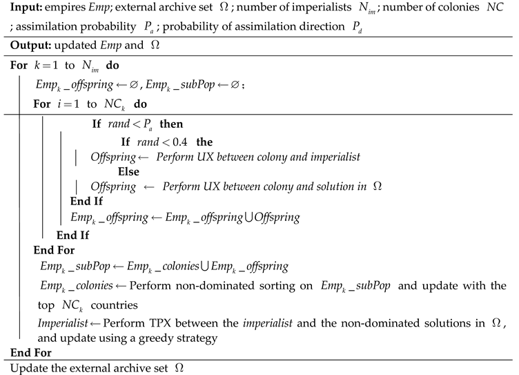
4.2. Assimilation Based on Q-Learning Adaptive Adjustment of Operator Parameter

Assimilation is the process by which colonies within an empire are moved towards the imperialist, with population evolution achieved through the assimilation of colonies by the imperialist. To ensure convergence speed while maintaining population diversity, a dynamic adaptive adjustment strategy for operator parameter based on Q-learning is designed. First, two different operator co-evolution operations are employed. Then, a Q-learning-based adaptive adjustment strategy for the UX operator parameter is implemented to enhance the convergence and diversity of the algorithm. Finally, an elite retention strategy is used to update the individuals of each empire, thereby improving the convergence speed. The pseudocode is shown in Algorithm 2.
Algorithm 2 Assimilation based on Q-learning adaptive adjustment of operator parameter
Preprints 116981 i002

4.2.1. Adaptive Adjustment of UX Operator Parameter Based on Q-Learning

During the assimilation process, the uniform crossover (UX) operator [21] and the two-point Crossover (TPX) operator [22] are used, respectively applied to the movement of colonies towards the imperialist and the external archive set. Among these, the UX operator is used as the main evolutionary operator to guide the evolutionary process of population and can also be applied for local search [21], playing an important role in the quality of population evolution. The parameter of the UX operator determines the number of high-quality genes passed from parents to offspring. In the early stages of evolution, a larger parameter is helpful for the algorithm converge, while in the later stages of evolution, a larger parameter can result in poor population diversity, causing the algorithm to fall into local optima. Therefore, a Q-learning-based adaptive adjustment strategy for the UX operator parameter is devised to dynamically adjust the evolutionary process of population, enabling the algorithm to converge more efficiently to the Pareto front.
State: The state of the entire population is determined by evaluating the convergence metric Δ G D of the non-dominated solution set compared to the reference set and the diversity metric Δ R a t i o , which represents the coverage ratio of the solution space. Here, Δ G D represents the generational distance difference of the non-dominated solutions obtained compared to the Pareto front P F * between generation t and t+1. P F * is a preset reference point, and Δ R a t i o represents the proportion of subregions occupied by the non-dominated solutions in the current generation in the objective space. The objective space is divided into several non-overlapping regions by weight vectors [23]. Δ G D indicates the degree of convergence of generation t+1 compared to generation t, the smaller the value of Δ G D , the better the convergence. Δ R a t i o represents the change in non-dominated set diversity, with Δ R a t i o < 0 indicating a decrease in diversity and Δ R a t i o > 0 indicating an increase in diversity. The calculations for Δ G D and Δ R a t i o are given by Equation (24) and Equation (25) respectively, where | P F t | and | ψ t | represent the number of non-dominated solutions in generation t and the proportion of the objective space they occupy. During the evolutionary, there are four possible states: (1) Δ G D > = 0 , Δ R a t i o > 0 ;(2) Δ G D > = 0 , Δ R a t i o < = 0 ;(3) Δ G D < 0 , Δ R a t i o > 0 ;(4) Δ G D < 0 , Δ R a t i o < = 0 .
Δ G D = ( x P F t + 1 min y P F * d ( x , y ) 2 / | P F t + 1 | ) ( x P F t min y P F * d ( x , y ) 2 / | P F t | )
Δ R a t i o = | ψ t + 1 | | ψ t |
Action: The action set A is composed of ten actions, representing ten levels of the UX operator parameter. By determining the current state of the population, the action with the highest Q-value in the Q-table is selected based on the ε-greedy strategy.
ε-greedy: In the initial iterations, Q-values usually lack prior knowledge, making it easy for the agent to fall into local optima during learning. Therefore, a ε-greedy strategy based on sigmod is used to guide the learning of agent. The mathematical expression for ε-greedy is as follows:
ε = 0.1 + ε 0.1 × 1 1 + e ( 0.2 × ( g 50 ) )
where g represents the number of iterations.
Reward: By calculating the values of Δ G D and Δ R a t i o after executing an action, the agent receives a corresponding reward and updates the Q-value of the action in the Q-table for the corresponding state according to Equation (27). If Δ G D 0 ,   Δ R a t i o > 0 , then reward = 1; if Δ G D 0 ,   Δ R a t i o < = 0 , then reward = -2; if Δ G D < 0 ,   Δ R a t i o > 0 , then reward = 4; if Δ G D < 0 ,   Δ R a t i o 0 , then reward = 2.
Q s t , a t ) = Q s t , a t ) + α [ r e w a r d t + 1 + γ max a A Q ( s t + 1 , a ) Q s t , a t ) ]
where α and γ are the learning rate and discount factor respectively, and A is the set of available actions.
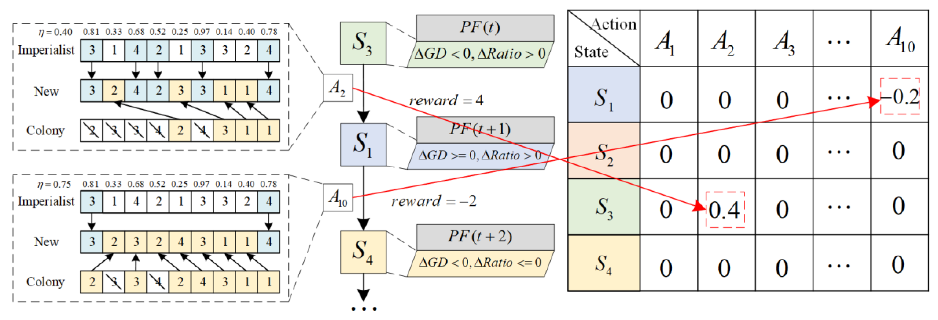
Figure 4 provides an example. In generation t, the population is in state S3 and the action A2 is chosen. After this action is executed, the population is transitioned to state S1 in generation t+1. In this state, the action A10 is chosen, and in generation t+2, the population is transitioned to state S4.

4.2.2. Update Strategy

To achieve rapid convergence of the population, an elite retention strategy is employed to select the colonies that need to be retained after the assimilation process. The specific operations are as follows: individuals generated during the assimilation process of imperialist I m p k are placed into the colony offspring population O f f s p r i n g k . After the assimilation operation within the empires is completed, the original colony population is merged with the colony offspring population to form a new population S u b P o p k . Then, the individuals in S u b P o p k are non-dominated sorted and their crowding distances are calculated. A number of N C k colonies are selected as the next generation of colonies. Additionally, for new solutions generated by the assimilation of the imperialist, if they are not dominated by the old solutions, the original imperialist is replaced by the new solutions; otherwise, no replacement is made.

4.3. Revolution Based on Hyper-Heuristic Variable Neighborhood Search

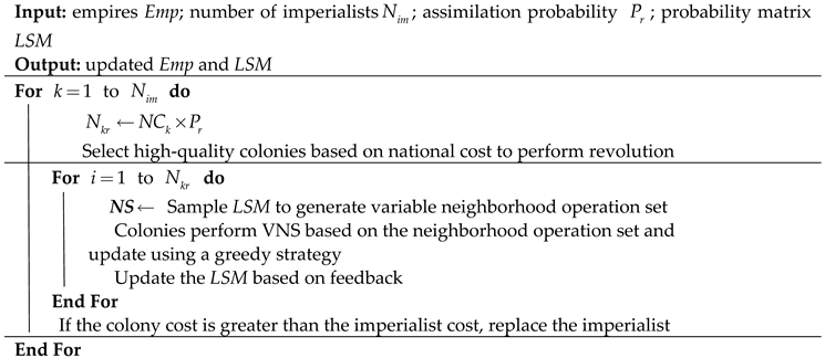
The colonial revolution is a process of further exploring and exploiting the neighborhood of superior colonies after completing the assimilation operation. In this paper, various neighborhood search (VNS) operations are designed, and high-level information constructed from a two-dimensional probability matrix is used to guide the selection of corresponding low-level variable neighborhood search operation sets. The selection of variable neighborhood search operators is dynamically adjusted by the high-level strategy based on the feedback information received from the environment after each application of the low-level variable neighborhood search operation set, thereby improving the search performance of the algorithm.

4.3.1. Neighborhood Search (NS) Operations
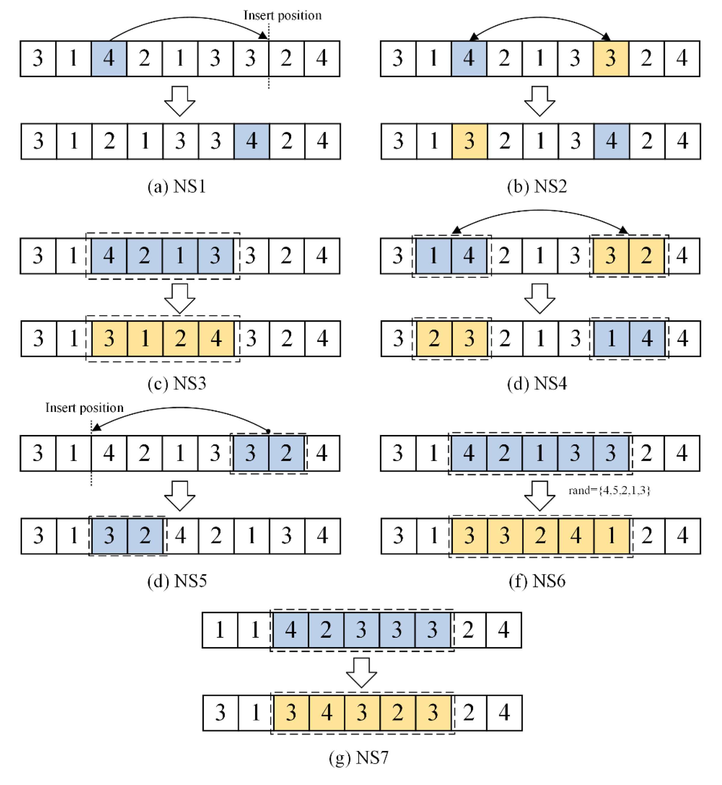
To implement an effective perturbation strategy for individuals, two single-operation-based neighborhood operations and five block-based neighborhood operations are designed as neighborhood search operators.
NS1: Single-operation insertion operation for individual encoding. A random operation is selected from the individual encoding and inserted into another position
NS2: Single-operation exchange operation for individual encoding. Two different operations are randomly selected and their positions are swapped.
NS3: Reversal operation for individual encoding. Two positions are randomly selected, and the segment of operations between these positions is reversed.
NS4: Segment exchange operation for individual encoding. Two segments of operations are randomly selected and their positions are exchanged.
NS5: Segment insertion operation for individual encoding. Two segments of operations are randomly selected and one segment is inserted into another position within the encoding.
NS6: Segment shuffling operation for individual encoding. A segment of operations is randomly selected, and operations within segment are randomly shuffled.
NS7: Segment gene dispersal operation for individual encoding. The individual encoding is divided into several segments, and the consecutive repeated genes within each segment are dispersed to different positions.
Figure 5. Schematic Diagram of Neighborhood Structure.
Preprints 116981 g005

4.3.2. Two-Dimensional Probability Model

Define N S = { N S G , k ( 1 ) , N S G , k ( 2 ) , , N S G , k ( l ) } as the neighborhood operations sequence executed by the k-th individual in generation G, where l represents the length of variable neighborhood search. The two-dimensional probability model P G ( x , y ) , shown in Equation (28), is used as the high-level strategy to guide the selection of the low-level the variable neighborhood search operations set.
P G ( x , y ) = [ P l × l G ( 1 , 1 )     P l × l G ( 1 , l ) P l × l G ( l , 1 )     P l × l G ( l , l ) ]
The initialization of the two-dimensional probability model and its update in the G-th generation are shown in Equation (29) and Equation (30) respectively.
P 0 ( x , y ) = 1 / l , x , y = 1 , 2 , , l
P G ( x , y ) = 1 + r e w a r d ) × P G 1 ( x , y ) , x = 1 , 2 , , l , y = N S ( 1 ) , N S ( 2 ) , , N S ( l )
r e w a r d = { 0.1 ,   new   solution   is   not   dominated   by   old   solution 0.1 ,   otherwise
After completing the revolution operations, the cost of each country within the empire is calculated, and the country with the highest cost is selected as the new imperialist, while the original imperialist becomes a colony. P G ( x , y ) is updated according to Equation (31).
Algorithm 3 Revolution based on hyper-heuristic variable neighborhood search
Preprints 116981 i003

4.4. Joint Imperialist Invasion

Dividing the population into multiple subpopulations is helpful for individuals to extensively search different areas, and balances the exploration and exploitation capabilities of the algorithm through co-evolution [24]. To address the issues of poor diversity and premature convergence in the basic Imperialist Competitive Algorithm, a joint imperialist competition mechanism is designed to replace the standard imperialist competition operations. Each empire is regarded as a population that collaboratively searches different regions of the solution space. This mechanism ensures that the collaborative evolutionary search is maintained within each empire and that information sharing and interaction are enhanced between empires, thereby improving diversity and the search efficiency of the algorithm.
The specific operations of the joint imperialist invasion are as follows: The total cost of each imperial group is calculated and ranked according to Equation (32), where E m p k represents the set of colonies owned by I m p k , and ξ is the proportional coefficient of the total cost of the empire accounted for by the colonies, which is set to 0.1. The imperialists of the top N i m 1 empires perform POX crossover [4] with random solutions, and the corresponding number of the worst colonies in the worst-ranked empire are replaced by the newly generated solutions. Through joint imperialist competition, the collaborative evolution within each empire can be maintained, while information sharing and interaction between empires can be enhanced, thus improving diversity and increasing the search efficiency of the algorithm.
T C k g = c i g + ξ σ E m p k c σ g / N C k
Algorithm 4 Joint imperialist invasion
Preprints 116981 i004

4.5. Algorithm Description

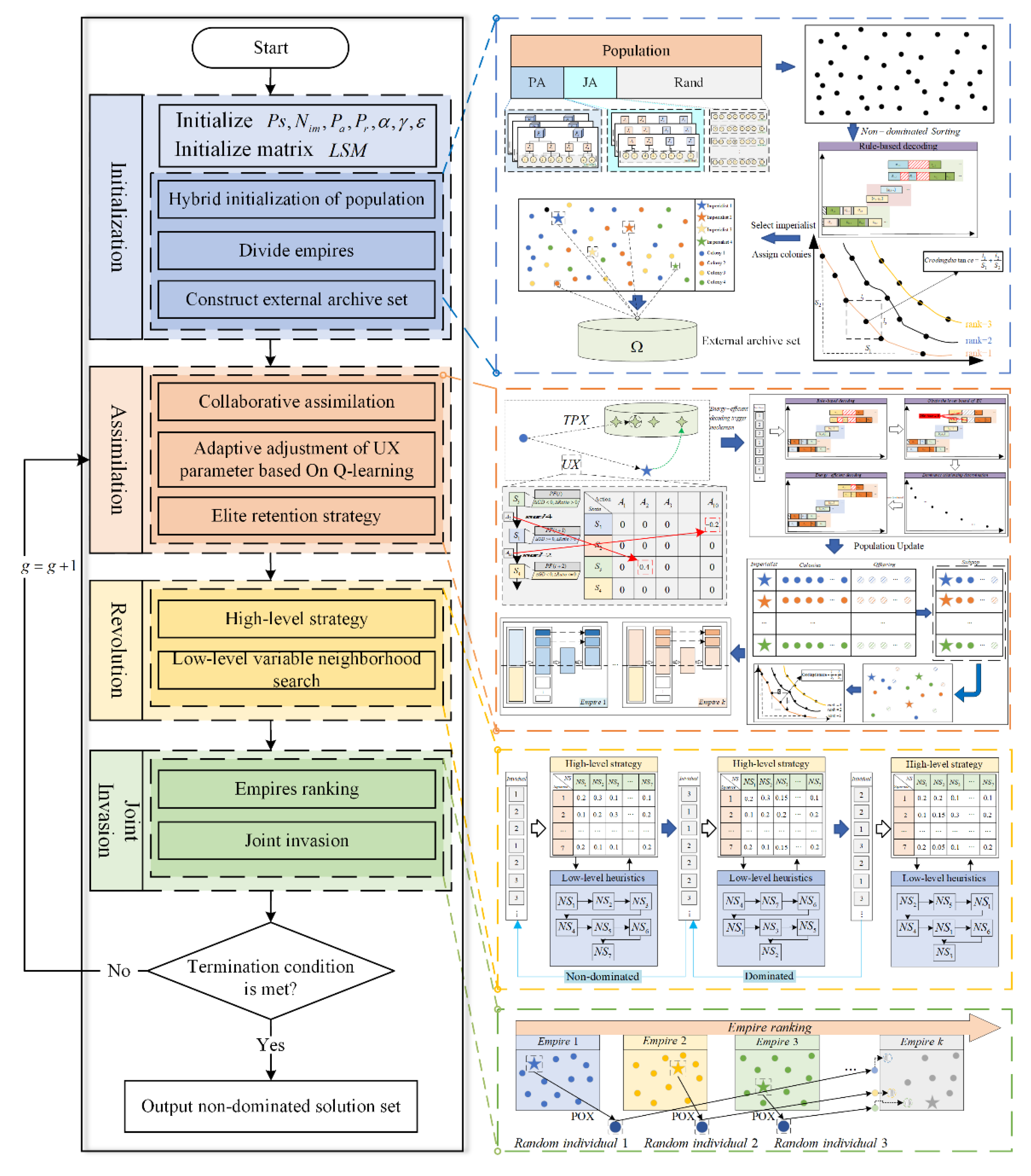
The flowchart of the proposed IICA-QL is shown in Figure 6. The process of IICA-QL is described as follows.
Step 1: Generate the initial population using heuristic rules and random generation methods. Select N i m imperialist countries to form the initial empires.
Step 2: Construct the external archive set and update it based on non-dominated solutions.
Step 3: Select UX operator parameter according to the Q-table, then perform assimilation in each empire and update Q-table. Meanwhile, retain colonies based on the elite retention strategy.
Step 4: Execute high-dimensional strategies constructed by the two-dimensional probability model to select low-level neighborhood search operations sequence. Update the probability model based on feedback information.
Step 5: Perform joint imperialist competition to achieve collaborative evolution of empires.
Step 6: If the termination condition is met, stop the search; otherwise, return to Step 3.

5. Experimental Results and Analysis

The proposed IICA-QL is implemented in MATLAB R2021a. The experimental configuration is an Intel Core i7-13700K and CPU @3.40GHz PC with 32GB memory. Since no prior research has been conducted on EEMsMlAJSP, the test data are generated randomly. The problem scale is denoted by O/J/A_M/T/K, where O/J/A represent the number of processing operations, jobs, and assembly operations, respectively. M/T/K represent the total number of processing machines, transport vehicles, and assembly machines, respectively. Detailed information about the product structure, order information, and production parameter data used in the experiments can be found from: https://github.com/captain-dyq/EEMsMlAJSP.git. The experimental time T ( i ) for each problem scale is determined based on the specific problem scale, where T ( i ) = O × M + J × T + A × K .

5.1. Performance Metrics

To comprehensively evaluate the convergence and diversity of the approximation Pareto fronts set obtained by the algorithm, the following three commonly used metrics are employed to measure the proposed IICA-QL.
(1)
Solution set Coverage (C-metric). This metric measures the dominance relationship between two solution sets, and is defined as follows:
C ( A , B ) = | x B | y A : y x | | B |
Where A and B are two non-dominated solution sets obtained by the algorithm. C(A,B) represents the proportion of solutions in set B that are dominated by at least one solution in set A. The larger the value of C(A,B), the better the performance of A.
(2)
Generational Distance (GD).
The proximity of the Pareto front PF obtained by the algorithm to the optimal Pareto front PF* is evaluated, where PF* is the true non-dominated solution set among the non-dominated sets obtained by all algorithms. For each solution x in PF, the nearest solution y in PF* is found, and their Euclidean distance is calculated. GD is the average of these shortest Euclidean distances, which is described as Equation (34). A smaller value of GD indicates better convergence and that the found PF is closer to the optimal Pareto front.
G D = x P F min d ( x , y ) 2 y P F * | P F |
(3)
Hypervolume (HV)
The HV metric is a univariate metric that represents the volume of the region in the objective space enclosed by the non-dominated solution set obtained by the algorithm and the reference point, which is set to (1.01,1.01) [25]. The hypervolume metric is a comprehensive metric for evaluating the convergence and diversity of the non-dominated solution set obtained by the algorithm. The larger the HV value, the better the overall performance of the algorithm.
H V ( E ) = L e b ( x E [ f 1 ( x ) , r 1 ] × ... × [ f m ( x ) , r m ] )
Where Leb(·) represents the Lebesgue measure and m represents the number of objectives in the problem.
To eliminate the impact of different dimensions, the solutions in the solution set are normalized according to the following formula [19]:
f i ' = f i f i min f i max f i min , i = 1 , 2

5.2. Parameter Settings

To determine the optimal values for the parameters in IICA-QL, the Design of Experiment (DOE) method is used for parameter setting. IICA-QL has a total of 7 parameters, each with three levels to choose from. The orthogonal array L27(37) is selected, and the meanings and optional parameter levels for each parameter are shown in Table 2. Experiments are conducted using a medium-sized experimental scale (82/42/71_3/3/3), with each parameter combination run 10 times and the runtime being T ( i ) = O × M + J × T + A × K . The hypervolume (HV) metric is calculated after each run for each parameter combination, and the average of the ten HV values is used as the response value (RV). Additionally, the average RV and influence of each parameter level are shown in Table 3. According to Table 3, the optimal parameter set is P s = 100, Nim = 3, Pa = 0.8, P r = 0.1, α = 0.2, γ = 0.9, ε = 0.6.

5.3. Effectiveness of the Adaptive Trigger Mechanism for the Energy-Efficient Strategy

To verify the effectiveness of the adaptive trigger mechanism for the energy-efficient strategy, IICA-QL (denoted as A) is compared with IICA-QL executing the energy-efficient strategy on Pareto solutions (IICA-QL-PFE, denoted as B) and IICA-QL executing the energy-efficient strategy on all individuals (IICA-QL-AE, denoted as C). Using the same computation time as the termination condition, each algorithm runs independently 10 times on 18 test instances. The average values of C-metric, GD, and HV obtained are shown in Table 4, with the best value for each metric highlighted in bold. The runtime of each algorithm on each scale is recorded in Table 5.
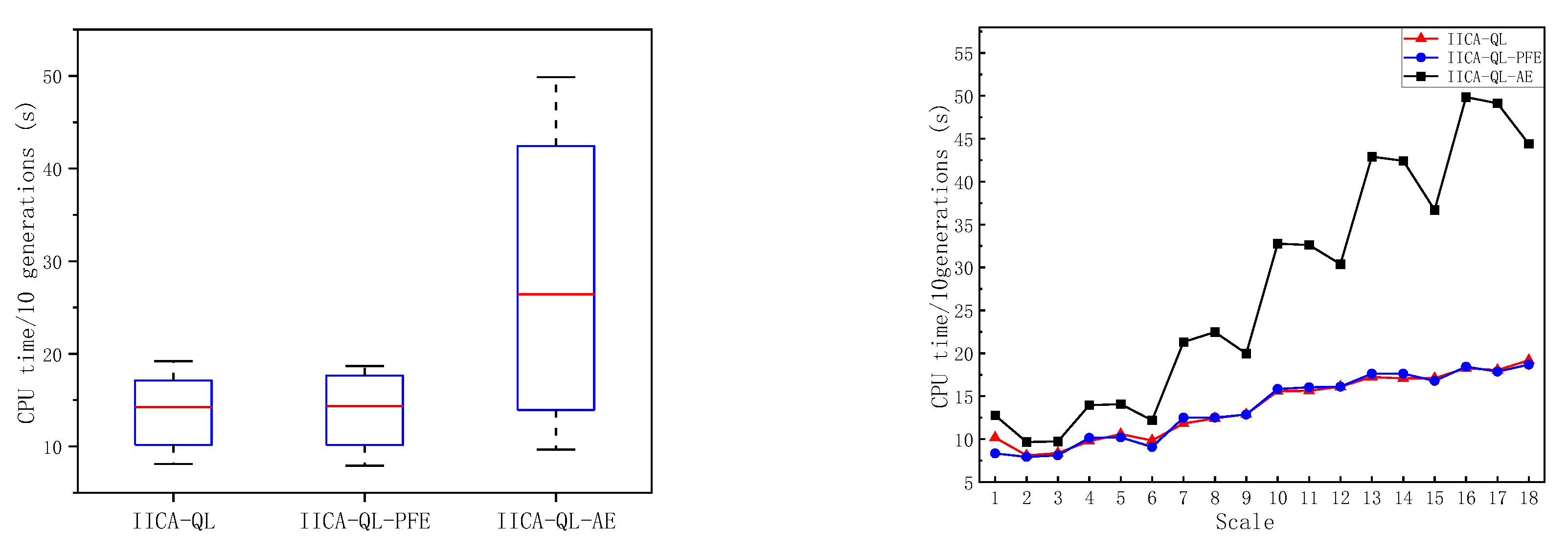
From the C-metric results in Table 4 and Figure 7, it can be seen that in all 18 test instances, C(A,B) is greater than C(B,A), and in 17 instances, C(A,C) is greater than C(C,A). This indicates that the non-dominated solutions obtained by IICA-QL generally dominate those obtained by IICA-QL-PFE and IICA-QL-AE. From the GD and HV metrics, it is evident that in most test instances, the values for IICA-QL are better than those for IICA-QL-PFE and IICA-QL-AE, and the values for IICA-QL-AE are better than those for IICA-QL-PFE. This shows that the adaptive trigger mechanism for the energy-efficient strategy improves the search quality of the algorithm. Additionally, from Table 5 and Figure 8, it can be seen that the CPU time of IICA-QL is comparable to that of IICA-QL-PFE and significantly better than that of IICA-QL-AE, indicating that the adaptive trigger mechanism for the energy-efficient strategy improves the search efficiency of the algorithm. Therefore, the adaptive trigger mechanism for the energy-efficient strategy effectively enhances the performance of the algorithm.

5.4. Effectiveness of Operator Parameter Adaptive Adjustment Based on Q-Learning

To verify the effectiveness of dynamic adaptive adjustment of operator parameter based on Q-learning, IICA-QL (denoted as A) is compared with IICA-QL without this strategy (IICA-nQL, denoted as B), where the UX parameter is set to 0.55. Using the same computation time as the termination condition, each algorithm runs independently 10 times on 18 test instances. The average values of C-metric, GD, and HV obtained are shown in Table 6, with the best value for each metric highlighted in bold.
From the C-metric results in Table 6 and Figure 9, it can be seen that in 17 out of 18 test instances, C(A,B) is greater than C(B,A), and C(A,B) shows an increasing trend. This indicates that the non-dominated solutions obtained by IICA-QL generally dominate those obtained by IICA-nQL, and the advantage becomes more pronounced as the problem scale increases. From the GD and HV metrics, it is evident that in all test instances, the values for IICA-QL are better than those for IICA-nQL, indicating that IICA-QL has better convergence and diversity compared to IICA-nQL. Therefore, the dynamic adaptive adjustment strategy for operator parameter based on Q-learning effectively enhances the performance of the algorithm.

5.5. Comparison with Other Algorithms

Since no existing research has been conducted on solving EEMsMlAJSP, to verify the effectiveness of the algorithm, IICA-QL is compared with algorithms BPBMO [22], PSO-GA[26], and KBOA [17], which solve similar problems to EEMsMlAJSP. The parameters for BPBMO, PSO-GA, and KBOA are chosen as specified in their respective references. Each of the four algorithms is independently run 10 times for the runtime determined by the problem scale, and the average values of the evaluation metrics are calculated. The C-metric, GD, and HV values for each algorithm across 18 problem scales are shown in Table 7 and Table 8, with the best value for each metric highlighted in bold.
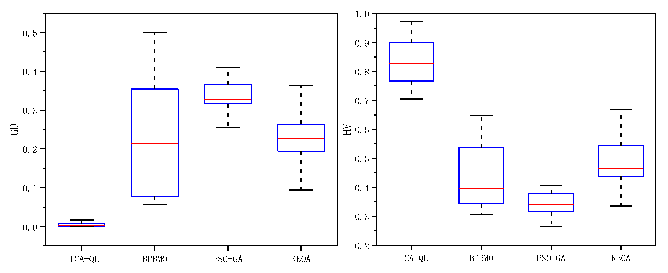
As seen in Table 7 and Figure 10, the GD and HV values obtained by IICA-QL are superior to those of BPBMO, PSO-GA, and KBOA in all test instances. Specifically, the performance of IICA-QL in terms of the GD metric indicates that it can find solutions very close to the Pareto optimal front in the solution space, demonstrating a significant advantage in convergence. From the HV metric, it is evident that the values obtained by IICA-QL are much higher than those of the other three algorithms, indicating that IICA-QL not only finds high-quality solutions but also maintains solution diversity, covering a broader Pareto front region. Therefore, the effectiveness of IICA-QL in solving EEMsMlAJSP is validated.
To further illustrate the performance of the compared algorithms, Figure 11 presents the Pareto results obtained by four algorithms on small, medium, and large-scale instances, respectively. As shown in the figure, the Pareto front obtained by IICA-QL outperforms those of the other three algorithms across different instances, indicating that IICA-QL is able to achieve non-dominated solutions with lower C max and TEC compared to BPBMO, PSO-GA, and KBOA.

6. Conclusions

This study has addressed the multi-stage, multi-level assembly job shop scheduling problem, aiming to minimize the maximum completion time and total energy consumption. An improved imperialist competitive algorithm based on Q-learning (IICA-QL) has been proposed. First, the EEMsMlAJSP problem model has been established. Second, encoding and decoding strategies based on the problem's characteristics have been designed, and an energy-saving decoding strategy trigger mechanism has been proposed to improve solution quality and search efficiency. Then, a dynamic adaptive adjustment strategy for the assimilation operator parameter has been achieved through Q-learning, enhancing convergence speed while ensuring population diversity. Finally, Experimental results have demonstrated the effectiveness of the proposed algorithm.
Future research will further consider the following aspects: (1) incorporating more complex constraints and optimization objectives widely present in actual production to make the problem model more aligned with real production needs; (2) applying other algorithms to solve EEMsMlAJSP, combining optimization algorithms with machine learning techniques to enhance algorithm performance; (3) improving the diversity of the algorithm's search to provide a better-distributed non-dominated solution set.

Author Contributions

Conceptualization, Y.D. and W.L.; methodology, Y.D. and W.L.; software, Y.D.; formal analysis, Y.D., W.L. and G.X.; investigation, Y.D., W.L. and G.X.; resources, W.L.; data curation, Y.D., W.L. and G.X.; writing—original draft preparation, Y.D.; writing—review and editing, Y.D., and W.L.; visualization, G.X.; supervision, W.L.; project administration, Y.D. and W.L.; funding acquisition, W.L.; All authors have read and agreed to the published version of the manuscript.

Funding

This research was funded by the "Revealing the Leaders" list of Chengdu Science and Technology Project (NO: 2023-JB00-00020-GX).

Institutional Review Board Statement

Not applicable.

Informed Consent Statement

Not applicable.

Data Availability Statement

The data presented in this study are openly available in GitHub at https://github.com/captain-dyq/EEMsMlAJSP.git.

Acknowledgments

We would like to sincerely thank Mr. Bizhen Bao and Mr. Weigang Xu from Chengdu SIWI High-tech Industry Co., LTD. for their significant support in this research. They played crucial roles in investigation, data acquisition, and analysis. Additionally, they made important contributions to the review and refinement of the manuscript, providing valuable feedback that enhanced the quality of the final paper.

Conflicts of Interest

The authors declare no conflicts of interest.

References

  1. Wang J, Lei D, Cai J. An adaptive artificial bee colony with reinforcement learning for distributed three-stage assembly scheduling with maintenance. Appl Soft Comput. 2022;117:108371. [CrossRef]
  2. Cheng L, Tang Q, Liu S, Zhang L. Mathematical model and augmented simulated annealing algorithm for mixed-model assembly job shop scheduling problem with batch transfer. Knowl-Based Syst. 2023;279:110968. [CrossRef]
  3. Cheng L, Tang Q, Zhang L. Production costs and total completion time minimization for three-stage mixed-model assembly job shop scheduling with lot streaming and batch transfer. Eng Appl Artif Intell. 2024;130:107729. [CrossRef]
  4. Gong G, Chiong R, Deng Q, et al. A two-stage memetic algorithm for energy-efficient flexible job shop scheduling by means of decreasing the total number of machine restarts. Swarm Evol Comput. 2022;75:101131. [CrossRef]
  5. Wang JJ, Wang L. A Cooperative Memetic Algorithm With Learning-Based Agent for Energy-Aware Distributed Hybrid Flow-Shop Scheduling. IEEE Trans Evol Comput. 2022;26(3):461-475. [CrossRef]
  6. Cao S, Li R, Gong W, Lu C. Inverse model and adaptive neighborhood search based cooperative optimizer for energy-efficient distributed flexible job shop scheduling. Swarm Evol Comput. 2023;83:101419. [CrossRef]
  7. Wang J jing, Wang L. A cooperative memetic algorithm with feedback for the energy-aware distributed flow-shops with flexible assembly scheduling. Comput Ind Eng. 2022;168:108126. [CrossRef]
  8. Li R, Gong W, Wang L, Lu C, Zhuang X. Surprisingly Popular-Based Adaptive Memetic Algorithm for Energy-Efficient Distributed Flexible Job Shop Scheduling. IEEE Trans Cybern. Published online 2023:1-11. [CrossRef]
  9. Meng L, Zhang C, Zhang B, Gao K, Ren Y, Sang H. MILP modeling and optimization of multi-objective flexible job shop scheduling problem with controllable processing times. Swarm Evol Comput. 2023;82:101374. [CrossRef]
  10. Lei D, Li M, Wang L. A Two-Phase Meta-Heuristic for Multiobjective Flexible Job Shop Scheduling Problem With Total Energy Consumption Threshold. IEEE Trans Cybern. 2019;49(3):1097-1109. [CrossRef]
  11. Zhou R, Lei D, Zhou X. Multi-Objective Energy-Efficient Interval Scheduling in Hybrid Flow Shop Using Imperialist Competitive Algorithm. IEEE Access. 2019;7:85029-85041. [CrossRef]
  12. Lei D, Yuan Y, Cai J, Bai D. An imperialist competitive algorithm with memory for distributed unrelated parallel machines scheduling. Int J Prod Res. 2020;58(2):597-614. [CrossRef]
  13. Li Y, Yang Z, Wang L, Tang H, Sun L, Guo S. A hybrid imperialist competitive algorithm for energy-efficient flexible job shop scheduling problem with variable-size sublots. Comput Ind Eng. 2022;172:108641. [CrossRef]
  14. Chen Y, Zhong J, Mumtaz J, Zhou S, Zhu L. An improved spider monkey optimization algorithm for multi-objective planning and scheduling problems of PCB assembly line. Expert Syst Appl. 2023;229:120600. [CrossRef]
  15. Chen R, Yang B, Li S, Wang S. A self-learning genetic algorithm based on reinforcement learning for flexible job-shop scheduling problem. Comput Ind Eng. 2020;149:106778. [CrossRef]
  16. Li R, Gong W, Lu C, Wang L. A Learning-Based Memetic Algorithm for Energy-Efficient Flexible Job-Shop Scheduling With Type-2 Fuzzy Processing Time. IEEE Trans Evol Comput. 2023;27(3):610-620. [CrossRef]
  17. Pan Z, Wang L, Wang J, Yu Y. Distributed Energy-Efficient Flexible Manufacturing With Assembly and Transportation: A Knowledge-Based Bi-Hierarchical Optimization Approach. IEEE Trans Autom Sci Eng. Published online 2024:1-17. [CrossRef]
  18. Zou P, Rajora M, Liang SY. A new algorithm based on evolutionary computation for hierarchically coupled constraint optimization: methodology and application to assembly job-shop scheduling. J Sched. 2018;21(5):545-563. [CrossRef]
  19. Zhu Z, Zhou X. An efficient evolutionary grey wolf optimizer for multi-objective flexible job shop scheduling problem with hierarchical job precedence constraints. Comput Ind Eng. 2020;140:106280. [CrossRef]
  20. Li M, Lei D, Cai J. Two-level imperialist competitive algorithm for energy-efficient hybrid flow shop scheduling problem with relative importance of objectives. Swarm Evol Comput. 2019;49:34-43. [CrossRef]
  21. Fontes DBMM, Homayouni SM, Fernandes JC. Energy-efficient job shop scheduling problem with transport resources considering speed adjustable resources. Int J Prod Res. 2023;0(0):1-24. [CrossRef]
  22. Li J, Han Y, Gao K, Xiao X, Duan P. Bi-Population Balancing Multi-Objective Algorithm for Fuzzy Flexible Job Shop With Energy and Transportation. IEEE Trans Autom Sci Eng. Published online 2023:1-17. [CrossRef]
  23. Ming M, Trivedi A, Wang R, Srinivasan D, Zhang T. A Dual-Population-Based Evolutionary Algorithm for Constrained Multiobjective Optimization. IEEE Trans Evol Comput. 2021;25(4):739-753. [CrossRef]
  24. Cheng L, Tang Q, Zhang L, Meng K. Mathematical model and enhanced cooperative co-evolutionary algorithm for scheduling energy-efficient manufacturing cell. J Clean Prod. 2021;326:129248. [CrossRef]
  25. Wang J jing, Wang L, Xiu X. A cooperative memetic algorithm for energy-aware distributed welding shop scheduling problem. Eng Appl Artif Intell. 2023;120:105877. [CrossRef]
  26. Ren W, Wen J, Yan Y, Hu Y, Guan Y, Li J. Multi-objective optimisation for energy-aware flexible job-shop scheduling problem with assembly operations. Int J Prod Res. 2021;59(23):7216-7231. [CrossRef]
Figure 1. A schematic diagram of the EEMsMlAJSP.
Preprints 116981 g001
Figure 2. Schematic diagram of Encoding.
Preprints 116981 g002
Figure 3. Illustration of the trigger mechanism for decoding energy-efficient strategy.
Preprints 116981 g003
Figure 4. Q-table update diagram.
Preprints 116981 g004
Figure 6. Framework of IICA-QL.
Preprints 116981 g006
Figure 7. Box plots of three metrics between IICA-QL and IICA-QL-PFE/IICA-QL-AE. .
Preprints 116981 g007
Figure 8. Box and line plots of CPU time between IICA-QL and IICA-QL-PFE/IICA-QL-AE.
Preprints 116981 g008
Figure 9. Box plots of three metrics between IICA-QL and IICA-nQL.
Preprints 116981 g009
Figure 10. Box plots of two metrics between IICA-QL and BPBMO/PSO-GA/ KBOA.
Preprints 116981 g010
Figure 11. The Pareto fronts obtained by IICA-QL, BPBMO, PSO-GA, KBOA with different scales.
Preprints 116981 g011
Table 2. Parameter Levels.
Parameter Notation Factor level
1 2 3
P s population size 50 100 150
Nim number of Imperialists 3 5 7
P a assimilation probability 0.7 0.8 0.9
P r revolutionary probability 0.1 0.2 0.3
α learning rate 0.1 0.2 0.3
γ discount factor 0.7 0.8 0.9
ε greed factor 0.3 0.6 0.9
Table 3. Average RVs and Ranks of each parameter.
Level P s P s P s P s P s P s P s
1 0.7855 0.7943 0.7786 0.7912 0.7868 0.7844 0.7851
2 0.7986 0.7814 0.7923 0.7838 0.7926 0.7856 0.7974
3 0.7786 0.7869 0.7917 0.7877 0.7832 0.7926 0.7801
Delta 0.0200 0.0130 0.0138 0.0074 0.0094 0.0083 0.0174
Rank 1 4 3 7 5 6 2
Table 4. Comparison results between IICA-QL and IICA-QL-PFE/IICA-QL-AE.
O/J/A_M/T/K C-metric GD HV
C(A,B) C(B,A) C(A,C) C(C,A) A B C A B C
25/13/22_2/2/2 0.3839 0.0400 0.2750 0.1600 0.0020 0.1062 0.0373 0.5436 0.5218 0.6807
25/13/22_3/2/2 0.6563 0.1050 0.2900 0.1409 0.0339 0.1394 0.0548 0.6450 0.5321 0.6181
25/13/22_3/3/3 0.4100 0.2100 0.3000 0.2000 0.0717 0.1468 0.1030 0.6490 0.5082 0.5965
44/23/39_2/2/2 0.5657 0.1820 0.3150 0.3000 0.0574 0.1509 0.0588 0.5470 0.3884 0.6212
44/23/39_3/2/2 0.4458 0.1650 0.3700 0.3450 0.0731 0.2145 0.1015 0.7129 0.3520 0.6705
44/23/39_3/3/3 0.5582 0.1350 0.3400 0.3133 0.1082 0.2129 0.0442 0.7045 0.3352 0.7143
82/42/71_2/2/2 0.4906 0.3996 0.5576 0.2904 0.1522 0.1231 0.1915 0.6359 0.5231 0.5631
82/42/71_3/2/2 0.7106 0.0514 0.4873 0.2845 0.0939 0.2222 0.0962 0.7420 0.4404 0.6939
82/42/71_3/3/3 0.4310 0.0681 0.2775 0.5630 0.1586 0.1963 0.0408 0.6667 0.2430 0.7947
135/70/120_3/3/3 0.4000 0.1630 0.5083 0.2593 0.0631 0.1542 0.0957 0.6700 0.3284 0.5469
135/70/120_4/3/3 0.2657 0.3518 0.4769 0.3038 0.1423 0.0738 0.1619 0.7283 0.6271 0.6485
135/70/120_4/3/4 0.3667 0.1672 0.5594 0.3510 0.0932 0.1349 0.1270 0.7616 0.4698 0.6264
173/88/151_3/3/3 0.6350 0.0258 0.7278 0.1113 0.0119 0.1721 0.1469 0.7686 0.1946 0.4786
173/88/151_4/3/3 0.6333 0.1595 0.8169 0.1060 0.0669 0.0912 0.2302 0.7864 0.4832 0.4958
173/88/151_4/3/4 0.3667 0.1445 0.7105 0.1496 0.0328 0.0415 0.1221 0.8258 0.5409 0.6232
202/104/175_3/3/3 0.4300 0.1385 0.3846 0.3389 0.0611 0.1018 0.0579 0.7153 0.2788 0.5539
202/104/175_4/3/3 0.4333 0.1494 0.8427 0.1018 0.0283 0.0734 0.1721 0.7675 0.4303 0.5742
202/104/175_4/3/4 0.4500 0.1076 0.6800 0.1413 0.0248 0.1309 0.0936 0.7295 0.2392 0.5453
Mean 0.4796 0.1535 0.4955 0.2478 0.0709 0.1381 0.1075 0.7000 0.4131 0.6137
Table 5. CPU time results of IICA-QL, IICA-QL-PFE and IICA-QL-AE.
O/J/A_M/T/K CPU time / 10 generations (s)
IICA-QL IICA-QL-PFE IICA-QL-AE
25/13/22_2/2/2 10.1695 8.3333 12.7660
25/13/22_3/2/2 8.1006 7.9235 9.6667
25/13/22_3/3/3 8.3721 8.1081 9.7297
44/23/39_2/2/2 9.7696 10.1435 13.9474
44/23/39_3/2/2 10.5785 10.1992 14.0659
44/23/39_3/3/3 9.8452 9.0857 12.1839
82/42/71_2/2/2 11.8182 12.5000 21.3115
82/42/71_3/2/2 12.4211 12.5199 22.4762
82/42/71_3/3/3 12.8855 12.8571 19.9659
135/70/120_3/3/3 15.5887 15.8373 32.7723
135/70/120_4/3/3 15.6354 16.0340 32.6225
135/70/120_4/3/4 16.1133 16.1133 30.3883
173/88/151_3/3/3 17.2385 17.6320 42.9167
173/88/151_4/3/3 17.0788 17.6345 42.4398
173/88/151_4/3/4 17.1053 16.7922 36.7059
202/104/175_3/3/3 18.2660 18.4342 49.8577
202/104/175_4/3/3 18.0452 17.8635 49.1385
202/104/175_4/3/4 19.1857 18.6786 44.3970
Mean 13.7898 13.7050 27.6306
Table 6. Comparison results between IICA-QL and IICA-nQL.
O/J/A_M/T/K C-metric GD HV
IICA-QL(A) IICA-nQL (B) IICA-QL IICA-nQL IICA-QL IICA-nQL
C(A,B) C(B,A)
25/13/22_2/2/2 0.3206 0.3050 0.0471 0.0585 0.6789 0.6848
25/13/22_3/2/2 0.3767 0.2617 0.0540 0.0669 0.6966 0.6940
25/13/22_3/3/3 0.3937 0.2950 0.0861 0.1289 0.7014 0.6438
44/23/39_2/2/2 0.3283 0.3679 0.0627 0.0633 0.7132 0.6424
44/23/39_3/2/2 0.3922 0.3344 0.0373 0.1339 0.7103 0.6975
44/23/39_3/3/3 0.5367 0.3250 0.0622 0.1823 0.7490 0.6484
82/42/71_2/2/2 0.5235 0.2410 0.0253 0.1227 0.7581 0.6368
82/42/71_3/2/2 0.4920 0.3293 0.0297 0.0703 0.7999 0.7471
82/42/71_3/3/3 0.4343 0.3915 0.0928 0.1081 0.7274 0.7228
135/70/120_3/3/3 0.6492 0.3096 0.0351 0.0767 0.7898 0.7387
135/70/120_4/3/3 0.5101 0.3000 0.0383 0.0632 0.7579 0.7362
135/70/120_4/3/4 0.5018 0.4549 0.0406 0.0647 0.7681 0.7496
173/88/151_3/3/3 0.5481 0.3214 0.0431 0.0605 0.7361 0.7087
173/88/151_4/3/3 0.6261 0.3101 0.0342 0.1021 0.7803 0.7031
173/88/151_4/3/4 0.4405 0.4014 0.0472 0.1128 0.8402 0.7989
202/104/175_3/3/3 0.5780 0.2200 0.0200 0.1030 0.7784 0.6613
202/104/175_4/3/3 0.6417 0.2254 0.0232 0.1256 0.8142 0.6995
202/104/175_4/3/4 0.6208 0.3661 0.0353 0.0846 0.8250 0.7784
Mean 0.4952 0.3200 0.0452 0.0960 0.7569 0.7051
Table 7. Comparison of GD and HV results for IICA-QL, BPBMO[22], PSO-GA[26] and KBOA[17].
O/J/A_M/T/K GD HV
IICA-QL BPBMO PSO-GA KBOA IICA-QL BPBMO PSO-GA KBOA
25/13/22_2/2/2 0.0028 0.2698 0.3198 0.2026 0.7888 0.4022 0.3688 0.5433
25/13/22_3/2/2 0.0174 0.1952 0.3166 0.2087 0.8628 0.5660 0.4059 0.5858
25/13/22_3/3/3 0.0021 0.4099 0.3654 0.2204 0.8997 0.3544 0.3958 0.5970
44/23/39_2/2/2 0.0034 0.3417 0.3449 0.2514 0.8786 0.3625 0.3508 0.4630
44/23/39_3/2/2 0.0017 0.4248 0.5155 0.3644 0.9560 0.4654 0.3790 0.5477
44/23/39_3/3/3 0 0.4992 0.3343 0.1943 0.9531 0.3060 0.3785 0.6688
82/42/71_2/2/2 0.0013 0.2599 0.4022 0.2959 0.8988 0.5376 0.3174 0.4242
82/42/71_3/2/2 0.0127 0.1507 0.3259 0.1707 0.8421 0.4690 0.3655 0.4644
82/42/71_3/3/3 0.0075 0.3547 0.3316 0.0941 0.7589 0.3434 0.3313 0.4765
135/70/120_3/3/3 0.0003 0.0777 0.3235 0.2528 0.7709 0.3298 0.2637 0.4445
135/70/120_4/3/3 0.0005 0.3859 0.4102 0.4588 0.9723 0.4449 0.3878 0.3356
135/70/120_4/3/4 0.0010 0.2352 0.4640 0.2639 0.9323 0.6075 0.3326 0.2695
173/88/151_3/3/3 0.0031 0.1326 0.2997 0.2859 0.8063 0.3339 0.3163 0.4845
173/88/151_4/3/3 0 0.0733 0.2559 0.1525 0.7225 0.3928 0.3541 0.4779
173/88/151_4/3/4 0.0117 0.0677 0.3560 0.2144 0.7672 0.6232 0.3032 0.3667
202/104/175_3/3/3 0 0.0676 0.2872 0.2337 0.8153 0.3370 0.2904 0.4662
202/104/175_4/3/3 0.0049 0.0878 0.2991 0.1570 0.7052 0.3648 0.2861 0.4667
202/104/175_4/3/4 0.0217 0.0575 0.3204 0.2630 0.7515 0.6474 0.3274 0.4378
Mean 0.0051 0.2273 0.3485 0.2380 0.8379 0.4382 0.3419 0.4733
Disclaimer/Publisher’s Note: The statements, opinions and data contained in all publications are solely those of the individual author(s) and contributor(s) and not of MDPI and/or the editor(s). MDPI and/or the editor(s) disclaim responsibility for any injury to people or property resulting from any ideas, methods, instructions or products referred to in the content.
Copyright: This open access article is published under a Creative Commons CC BY 4.0 license, which permit the free download, distribution, and reuse, provided that the author and preprint are cited in any reuse.
Prerpints.org logo

Preprints.org is a free preprint server supported by MDPI in Basel, Switzerland.

Subscribe

© 2024 MDPI (Basel, Switzerland) unless otherwise stated