Multiobjective Majority-minority Cellular Automata Algorithm (MOMmCAA) for Global and Engineering Design Optimization

Preprint

Article

Multiobjective Majority-minority Cellular Automata Algorithm (MOMmCAA) for Global and Engineering Design Optimization

Altmetrics

Downloads

Views

Comments

A peer-reviewed article of this preprint also exists.

Juan Carlos Seck-Tuoh-Mora^*

Ulises Hernandez-Hurtado,

Joselito Medina-Marín

Norberto Hernández-Romero

Liliana Lizárraga-Mendiola

Juan Carlos Seck-Tuoh-Mora^*

Ulises Hernandez-Hurtado,

Joselito Medina-Marín

Norberto Hernández-Romero

Liliana Lizárraga-Mendiola

This version is not peer-reviewed

Submitted:

02 September 2024

Posted:

03 September 2024

You are already at the latest version

Alerts

Abstract

When dealing with complex models in real situations, many optimization problems require using more than one objective function to represent the relevant characteristics of the system under consideration adequately. This is why multiobjective optimization algorithms that can deal with several objective functions are required in order to obtain reasonable results in an adequate processing time. This paper presents the multiobjective version of a recent metaheuristic algorithm that optimizes a single objective function, known as the Majority-minority Cellular Automata Algorithm (MmCAA), inspired by cellular automata operation. The algorithm presented here will be known as the Multiobjective Majority-minority Cellular Automata Algorithm (MOMmCAA). The MOMmCAA adds repository management and multiobjective search space density control to complement the performance of the MmCAA and make it capable of optimizing multiobjective problems. To evaluate the performance of the MOMmCAA, benchmark test sets are taken (DTLZ, quadratic, and CEC-2020), along with real-world engineering design problems, compared against other multiobjective algorithms recognized for their performance (MOLAPO, GS, MOPSO, NSGA-II, and MNMA). The results obtained in this work show that MOMmCA produces comparable performance with the other metaheuristic methods, which shows it as a competitive algorithm to be used for multiobjective problems. MOMmCAA was implemented in MATLAB, and its source code can be consulted in GitHub. https://github.com/juanseck/MOMmCAA

Keywords:

Subject: Computer Science and Mathematics - Other

1. Introduction

Many real-world problems in engineering and other research areas require multiobjective optimization where it is necessary to find in the search space a set of solutions well distributed along the Pareto-optimal front. Generally, in this type of problem, the computation of possible solutions must consider the existence of two or more conflicting objective functions. A multiobjective optimization problem can be defined as:

\begin{matrix} min h (z) = (h_{1} (z), h_{2} (z), \dots, h_{m} (z)) \\ where z \in Q, m \geq 2 \end{matrix}

(1)

where each

h (z)

is a real-valued scalar function,

h (z)

is the set of objective or cost functions that when evaluated produce an m-dimensional vector in the

R^{m}

-objective space,

z = (z_{1}, z_{2}, \dots, z_{n})

is an n-dimensional vector in the search space

R^{n}

and

Q \subseteq R^{n}

is the set of all feasible solutions of Eq. 1.

In this type of problem, identifying the set of best possible solutions can, in many cases, be highly complicated or impossible. Rather than looking for globally optimal solutions to a multiobjective problem, one seeks to compute satisfactory solutions that can be obtained in adequate time, mainly to find the Pareto optimal (PS) set of solutions. The mapping from the PS to the objective space is the Pareto front (PF).

Multiobjective optimization evolutionary algorithms (MOEAs) are highly suitable for solving problems involving multiple objectives because they can generate a set of PF-approximate solutions in a single run [1]. In recent decades, many multiobjective optimization algorithms have been derived from classical single-objective metaheuristics, showing efficiency and effectiveness on various complex problems. Single-objective metaheuristics are optimization techniques that focus on finding a single optimal solution. Common examples include genetic algorithms (GA) [2], particle swarm optimization (PSO) [3], ant colony optimization (ACO) [4], or simulated annealing (SA) [5].

Several techniques based on single-objective metaheuristics have been developed to address multiobjective problems. Examples of the most outstanding ones are the Non-Dominated Sorting Genetic Algorithm (NSGA-II) which extends GAs to handle multiple objectives using a non-dominated sorting scheme and population diversity [6], the Multiobjective Evolutionary Algorithm Based on Decomposition (MOEA/D) which splits a multiobjective problem into several single-objective problems [7], the SPEA2 which uses a list of non-dominated solutions and assigns strengths to each solution to guide the search process [8], the Multiobjective PSO (MOPSO) which is an extension of the PSO handling multiple objectives while maintaining an archive of non-dominated solutions [9], the Multiobjective ACO (MOACO) which adapts the ACO for multiobjective optimization using multiple populations to improve computational efficiency [10,11], MOACO was also employed to address multiobjective problems in airline crew turnover [12] and to improve the configuration of a supply chain [13]. Multiobjective Simulated Annealing (MOSA) extends simulated annealing to handle multiple targets, maintaining a balance between exploration and exploitation [14], the Multiobjective Ant Lion Optimizer (MOALO) which expands the Ant Lion Optimizer by applying a repository to store non-dominated solutions in the Pareto set [15], the Multiobjective Multi-Verse Optimizer (MOMVO) which builds on the MVO to compare and optimize test and practical problems [16].

Another work that is an extension of a recent metaheuristic algorithm is the Multiobjective Salp Swarm Algorithm (MSSA) [17] inspired by the swarming behavior of sea salps, the MSSA splits the population into a leader and followers, using an external file to store the non-dominated solutions, showing adequate convergence and coverage of the PS. The interplay of several PSO algorithms for simultaneous optimization of single objectives in a multiobjective problem (MPMO) is described in [18] using multiple populations. In discrete problems, a new algorithm with multiple populations inspired by the GA is the MPMOGA, which solves the job-shop scheduling problem with multiple objectives, obtaining satisfactory results [19]. Based on the Heat Transfer Search, in [20], the Multi-Objective Heat Transfer Search (MOHTS) is proposed to optimize structural multiobjective problems, obtaining better results compared with other algorithms based on ant colonies and symbolic organisms. Speaking of the symbolic organism algorithm, the multiobjective version of the algorithm is presented in [21] for optimal reinforcement design.

The Multiobjective Teaching-Learning-based Optimization (MOTLBO) is an extension of the Teaching-Learning-based Optimization (TLBO) algorithm that uses two main phases: the teacher phase, where solutions are improved based on the best individual, and the learner phase, where solutions are optimized through knowledge sharing between individuals [22], the Multiobjective Thermal Exchange Optimization (MOTEO) is inspired by the principles of thermodynamics and heat exchange to solve optimization problems by considering multiple criteria simultaneously [23], the Multiobjective Plasma Generation Optimization (MOPGO) that takes up the generation and behavior of plasma where charged particles interact and move towards lower energy states [24], the Multiobjective Crystal Structure Algorithm (MOCSA) motivated by the formation and organization of crystalline structures; solutions resemble atoms that organize themselves into configurations that minimize the energy of the system [25], the Multiobjective Forest Optimization Algorithm (MOFOA) takes the dynamics and ecology of forests where solutions resemble trees competing for resources allowing the solutions (trees) to evolve and adapt in a competitive and cooperative environment [26], the Competitive Mechanism Integrated Multi-objective Whale Optimization Algorithm with Differential Evolution (CMI-MOWOA-DE) combines whale social behavior and differential evolution, the solutions simulate whale movement and hunting strategy, while differential evolution introduces variation and diversification to achieve a balance between multiple conflicting objectives, the Multi-objective Harris Hawks Optimizer (MOHHO) is an extension of the Harris Hawks Optimizer (HHO) algorithm that evokes the cooperative hunting strategies of Harris hawks [27], the Marine Predators Algorithm for multiobjective optimization (MPA) emulates the behavior of species such as sharks and dolphins, using search tactics and solution space exploitation to optimize multiple objectives [28], the multiobjective Sine-Cosine Algorithm (MOSCA) is a variant of the Sine-Cosine Algorithm (SCA) that uses sine and cosine functions to guide the exploration and exploitation of the search space, dynamically adjusting the positions of candidate solutions to maintain diversity and ensure convergence to the FP [29], the Multiobjective Atomic Orbital Search (MAOS) algorithm is based on the concept of atomic orbitals from quantum chemistry, the potential solutions are treated as electrons in different orbitals, and the search process resembles the movement of these electrons to reach lower energy configurations [30], the branch-and-bound framework for continuous global multiobjective optimization, where the search space is recursively divided into smaller subregions and lower and upper bounds are computed for the objective functions in these subregions; subregions that cannot contain optimal solutions are discarded, which reduces the overall search space, Multiobjective Differential Evolution (MODE) uses a population of candidate solutions that evolve through mutation operators, The Multiobjective optimization method based on adaptive parameter harmony search algorithm simulates the improvisation process of musicians searching for the best harmony, dynamically adapting its parameters using memory and tuning operators to explore new solutions and preserve the best ones found [31], the Guided Population Archive Whale Optimization Algorithm (GPA-WOA) is a variant of the Whale Optimization Algorithm (WOA) that simulates the hunting behavior of humpback whales and uses guides, or benchmark solutions, to direct the search and improve convergence to the FP; in addition, a population file is dynamically updated to preserve diversity and ensure that solutions are optimal and well-distributed [32], the Decomposition Based Quantum Inspired Quantum Salp Swarm Algorithm (DQSSA) combines quantum mechanical principles with the swarming behavior of salps, dividing the multiobjective problem into more tractable subproblems, allowing a set of well-distributed optimal solutions to be found at the FP [33].

The above works are just a sample of how many recent single-objective algorithms have been extended in various ways to deal with multiobjective problems. Single-objective optimization algorithms inspired by cellular automata [34,35,36,37,38] are practical and have competitive results on these types of problems compared to more recent metaheuristics. However, few works have applied the concept of cellular automata for general multiobjective optimization [39,40,41,42].

Following this trend, a recent single-objective optimization algorithm is the Majority-minority Cellular Automata Algorithm (MmCAA), which was tested on several test problems in multiple dimensions and for various applications in engineering, obtaining satisfactory results against other well-recognized algorithms [43]. This paper presents the multiobjective version of this algorithm called MOMmCAA. This algorithm is also inspired by the local behavior of cellular automata, particularly the majority and minority rules, which are intermixed and able to generate complex behaviors and perform the tasks of exploration and exploitation in the search space.

To test the performance of the MOMmCAA, the DLTZ benchmark, 10 quadratic problems, and 10 CEC2020 problems are taken. The proposed algorithm is also tested on 2 engineering problems, obtaining satisfactory results. In these cases, five other algorithms are considered for comparison, the Multiobjective Lightning Attachment Procedure Optimization (MOLAPO) [44], the Grid Search (GS) [45], the Multiobjective Particle Swarm Optimization (MOPSO) [9], the Non-dominated Sorting Genetic Algorithm (NSGA-II) [6] and the Multiobjective Nelder-Mead Algorithm (MNMA) [46].

A non-parametric Wilcoxon statistical test is performed to show the statistical significance of the experiments. The results show that the proposed algorithm is among the best-ranked compared to the other methods used in this work.

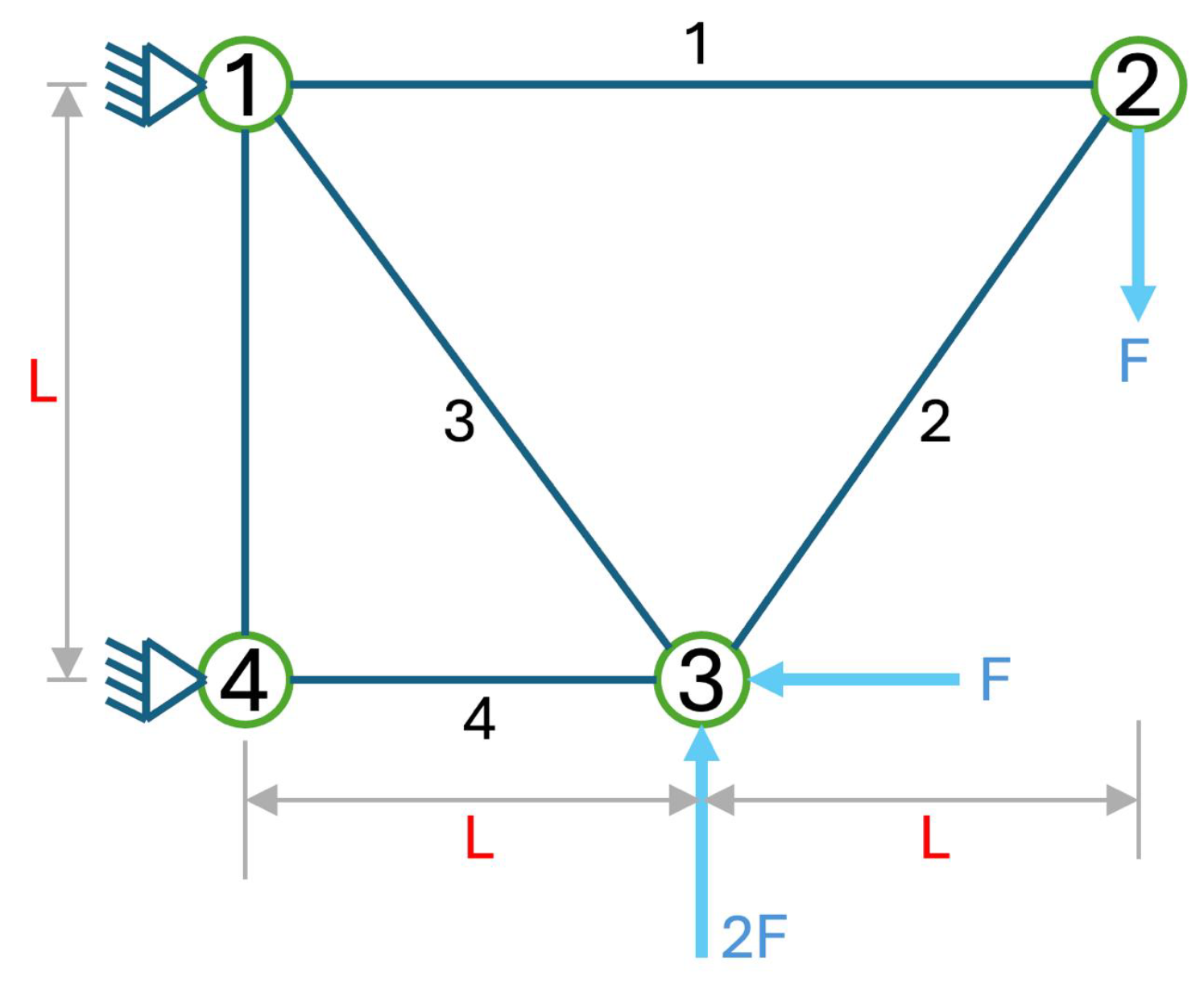
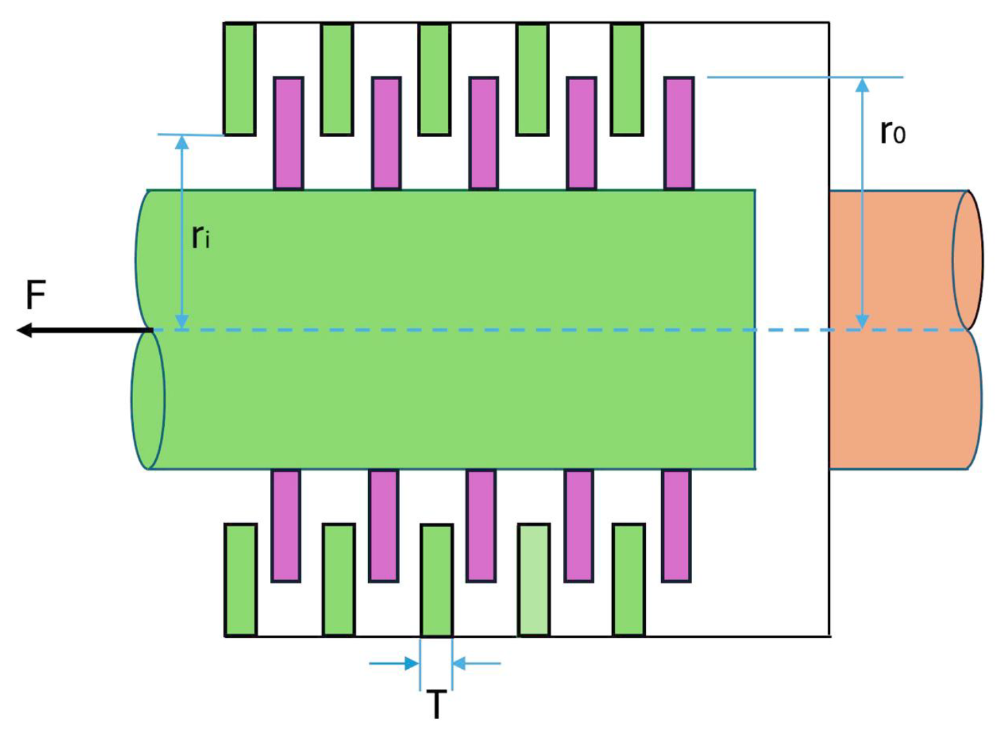
The rest of the article is organized as follows. Section 2 shows the Multiobjective Majority-minority Cellular Automata Algorithm (MOMmCAA) details. Section 4 presents the experiments of MOMmCAA on various test benches (DTLZ benchmark, 10 quadratic problems, and 10 CEC2020 problems), comparing it statistically through the Wilcoxon test against other multiobjective algorithms recognized for their performance. Section describes the application of MOMmCAA in engineering problems (four-bar truss and disk brake design problems). Finally, Section 6 gives the paper’s conclusions.

2. The Proposed Multiobjective Majority-minority Cellular Automata Algorithm (MOMmCAA)

This section briefly explains the concept of cellular automata, the general characteristics of the Majority-minority Cellular Automata Algorithm, and the multiobjective implementation of this algorithm. The concept of hypercubes is used to delimit a repository for managing the PS solutions generated by the algorithm.

3. Basic Concepts of Cellular Automata with Majority Rule

A cellular automaton (CA) is a dynamic system of cells that initially take a value from a finite set of possible states. The dynamics of the CA is in discrete steps, making it a discrete system in time and space. At each step, a cell considers its current state and that of its close neighbors to update its state at the next time step. In this way, a mapping from blocks of states to individual states is called an evolution rule. CAs can generate chaotic and complex global behaviors depending on the evolution rule that defines their local mapping. Because of this, CAs have been widely investigated and applied in various engineering and computational problems [47,48].

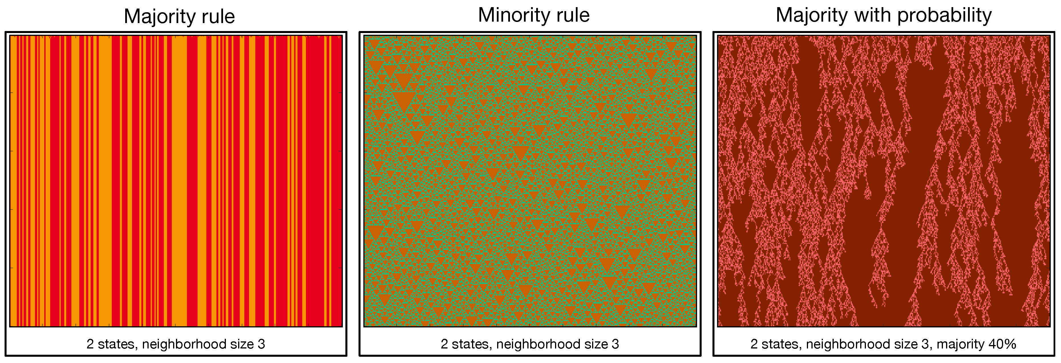
One of the rules of evolution extensively studied in recent work is the majority rule. In this rule, each cell takes its new state as the most common state in its local neighborhood. The dynamics of this rule is characterized by patchy patterns that stabilize as the system’s evolution progresses. Its counterpart is the minority rule, which takes the least common element of each neighborhood to update the state of a cell in the next generation. The evolution of the minority rule is characterized by the fact that it does not tend quickly to a fixed or periodic state because a minority state tends to become the majority and vice versa, resulting in oscillating global dynamics.

In Figure 1, we can see various dynamic behaviors of the majority rule, the minority rule, and the application of the majority rule with probability in cellular automata of two states and various neighborhood sizes. In these examples, 500 cells and 250 evolutions were used. Evolution generates a periodic pattern for the original majority rule, while the minority rule generates a chaotic pattern of heterogeneous triangular shapes. If the rules are alternated probabilistically, one has the formation of complex patterns where non-periodic structures are combined with a stable background.

This combination of majority and minority rules was used as inspiration to define the Majority-minority Cellular Automata Algorithm (MmCAA) algorithm for single-objective optimization [43]. The inspiration of MmCAA is to emulate the dynamic behavior of applying majority and minority rules in cellular automata.

The MmCAA starts by generating a random population S of

n_{S}

smart-cells, where each smart-cell is represented as

s \in R^{n}

. The dynamics of each

s

is defined by a set of rules, where one of them is chosen randomly to improve the position of the smart-cell. The rules take information from other smart-cells to generate new neighbors, from which the best one is selected to upgrade the smart-cell position. With this mechanism, the positions of all smart-cells in the population are improved, and the system evolves iteratively during the optimization process. The rules used by the MmCAA for smart-cell evolution are as follows.

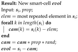
The Majority (minority) rule applied to a single smart-cell is described in Algorithm 1. The input is a smart-cell

s_{i}

for

1 \leq i \leq n_{S}

and a weight parameter

p r o p

that defines a limit on the change in the values of

s_{i}

. The rule takes the differences

b m c a m

between the values in

b m s_{i}

and the most repeated element

e l e m

in the smart-cell and

r a n d

generates a random value between 0 and 1. A new solution

evol

is formed by taking the differences between the original smart-cell and

cam

randomly weighted between 0 and

p r o p

. This rule helps to bring the values of

s_{i}

closer to the most repeated value

e l e m

Algorithm 1: Majority (minority) rule for a single smart-cell

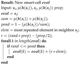
The Majority (minority) rule applied with a neighboring smart-cell is described in Algorithm 2. The most repeated value of a neighboring smart-cell

s_{j})

is taken as the change factor depending on the average weight of the neighbor cost

μ (h (s_{j}))

. If the cost

m u (h (s_{i}))

is larger than

m u (h (s_{j}))

, then the weight

p o n d

is large and there is a higher probability of changing

b m s_{i}

, by taking a random ratio between

- p r o p

and

p r o p

of the most repeated element in

b m s_{j}

and modifying each randomly selected position in

b m s_{i}

Algorithm 2: Majority (minority) rule with one neighbor

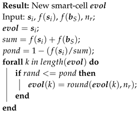
The rule for rounding values in a smart-cell (Algorithm 3) consists of rounding off the

n_{r}

to the most significant decimal values of the selected elements in

s_{i}

. The least significant decimal digit is the

n_{r}

-th digit to the right of the decimal point. The least significant digit remains unchanged if the first non-significant digit is less than 5. Otherwise, the least significant digit is incremented by 1. This rule is applicable for optimization problems to find proper parameters.

Algorithm 3: Rounding rule

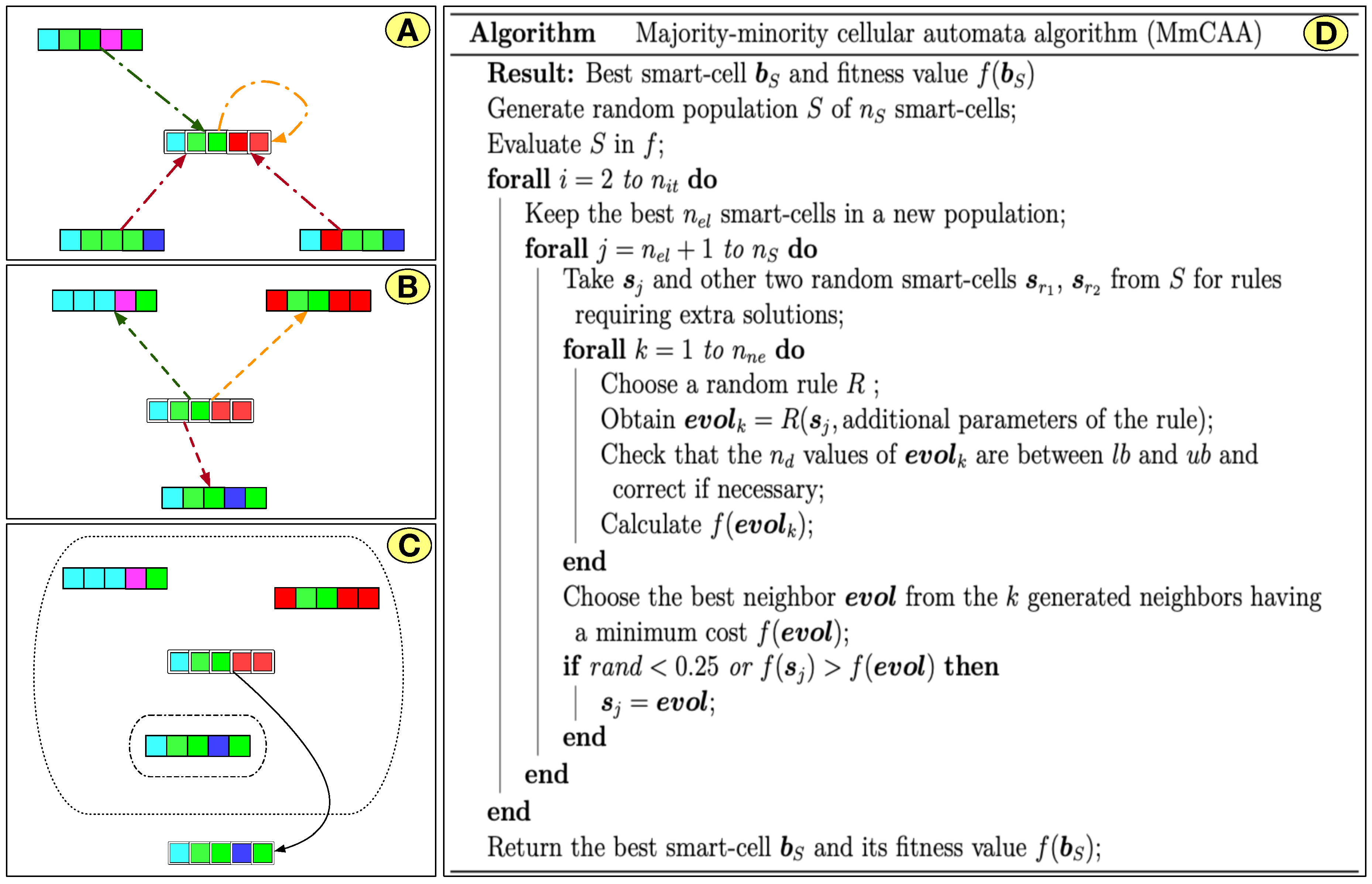
The adaptation of the majority and minority rules considers the elements of each solution that are repeated to a greater or lesser degree in the same smart-cell or in one or two additional smart-cells to obtain a new position. The randomness in choosing evolution rules and neighbors allows access to the information in the rest of the population, thus generating large and small changes in the position of a smart-cell, which favors the exploration and exploitation phases to escape from local optima and avoid the stagnation of the solutions. The MmCAA is presented in Figure 2. In (A), each smart-cell checks neighbors using different majority and minority rules. These rules produce new solutions (B), and the best solution in the neighborhood is selected to update the smart-cell (C). The pseudo-code of MmCAA is described in (D).

3.1. Multiobjective Majority-minority Cellular Automata Algorithm (MOMmCAA)

MmCAA was devised to solve single-objective optimization problems; therefore, it needs to be modified to deal with multiobjective problems. This results in the creation of the multiobjective variant MOMmCAA.

Taking as a basis the MmCAA inspired by the combination of majority and minority cellular automata and the handling of a solution repository on the Pareto front of the MOPSO algorithm, the MOMmCAA uses the following mechanisms for multiobjective optimization.

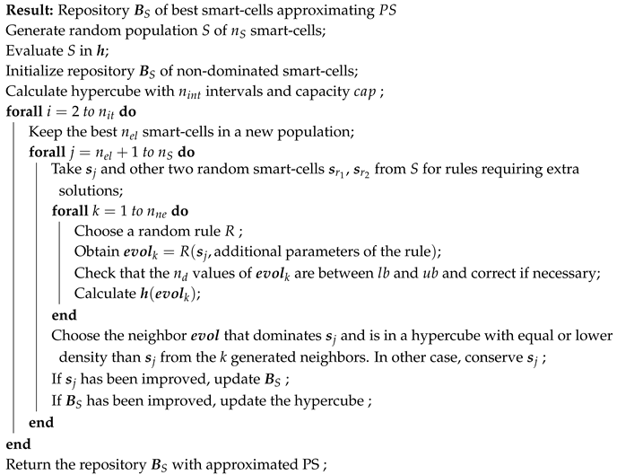
Update of each smart-cell: Each smart-cell solution generates a new set of neighboring solutions by taking its information or the information from one or two neighboring smart-cells depending on the evolution rule that is randomly selected. Some rules favor exploration by taking information from other smart-cells, and others the exploitation when they only take information contained in the same smart-cell. From this set of neighbors, the one that is not dominated by the rest is taken, and it will update the smart-cell if it dominates it.

Repository with non-dominated solutions: The non-dominated smart-cells are stored in a repository, which also serves as a file to take neighbors when applying the different evolution rules that define the MOMmCAA optimization process. For a smart-cell to enter the repository, it must dominate another solution, or any other solution in the repository does not dominate it. The repository has a limited capacity, and if a new smart-cell enters the repository, the smart-cell that is dominated or the one that is in a region of the objective space with high density is deleted.

Hypercube density management in the objective space: Taking inspiration from the MOPSO mechanism, solutions in the PS are ranked depending on the density of the hypercube in which they are found in the solution space. If any other solution in the repository does not dominate a new solution and, in turn, is in a hypercube of lower density, then a solution that is in the hypercube with higher density is removed from the repository. This allows the repository to have a better diversity of solutions. If a new solution is found in a new hypercube, then the boundaries of the solution space are expanded, and the hypercube densities are recalculated. 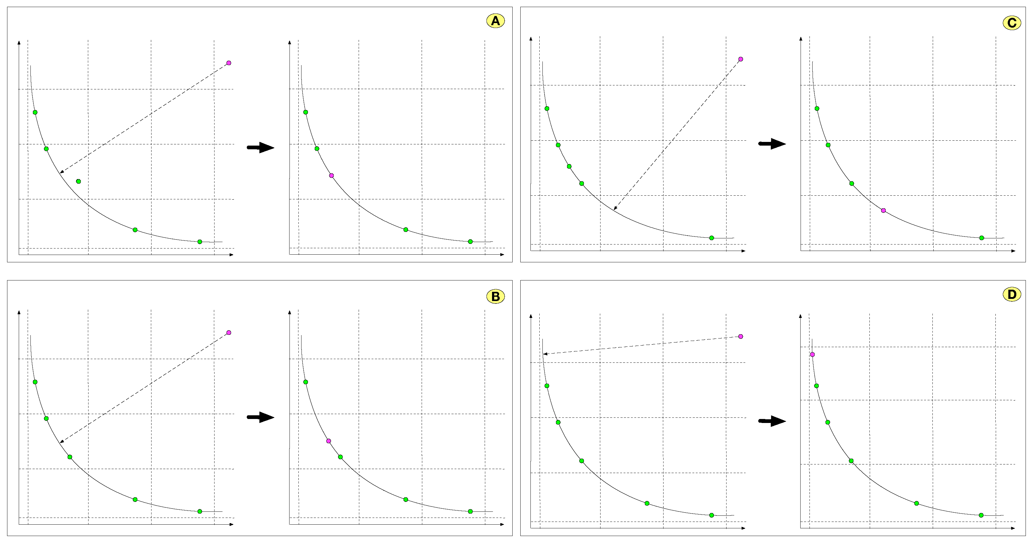Figure 3 shows the handling of smart-cell selection in the repository using hypercubes; in (A) a new smart-cell replaces another smart-cell in a hypercube if it dominates it. In (B), if the new smart-cell falls into a higher-density hypercube and the repository is complete, one of the smart-cells is randomly removed. In (C), if the new smart-cell falls into a less dense hypercube and the repository is complete, then one smart-cell is randomly removed from the denser hypercube. In (D), the hypercube boundaries are updated if the new smart-cell falls outside the current hypercube boundaries.

The pseudocode of the MOMmCAA is presented in Algorithm 4.

Algorithm 4: multiObjective Majority-minority Cellular Automata Algorithm (MmCAA)

The computational complexity of the MOMmCAA is

O (m N^{2})

where N is the number of smart-cells. One of the advantages of using adaptive hypercubes is that the computational cost is better than using a niche strategy such as the one used by NSGA-II [49]. The only case where both strategies have the same complexity is when the hypercubes are updated at each generation, obtaining the value of

O (N^{2})

[50]. Thus, the complexity of MOMmCAA is similar to that of MOPSO.

4. Computational Experiments to Compare MOMmCAA with Other Algorithms

MOLAPO, GS, MOPSO, NSGA-II, MOMVO, and MNMA were compared to MOMmCAA to identify the best performance in calculating Pareto optimal solutions. The initial parameters of all described algorithms are summarized in Table 1. Each experiment employed 50 PS solutions and a maximum of 1000 iterations. The proposed algorithm was tested in 29 diverse case studies, including 27 unconstrained and constrained mathematical problems and two real-world engineering design problems.

The original Matlab implementations of these algorithms were taken directly from the web addresses indicated in the reference articles. The Matlab code of MOMmCAA can be downloaded on Github from the link https://github.com/juanseck/MOMmCAA. MOMmCAA and the other algorithms were executed in Matlab 2015a on a

3.1

GHz Intel Xeon CPU and 64 GB in RAM with a macOS Sonoma operating system. 30 independent runs were made for each algorithm on every benchmark function. The metrics used to compare the results of the algorithms are as follows.

Hypervolume (HV): The diverseness in search space through the hypervolume metric is introduced by Ulrich et al. to escalate the diversity in both decision space and objective space [51]. The HV of a set of solutions measures the size of the portion of the objective space dominated by those solutions as a group. In general, HV is favored because it captures in a single scalar both the closeness of the solutions to the optimal set and, to some extent, the distribution of solutions across the objective space. It measures both convergence and diversity. The HV value can be calculated using the below equation.

H V = \cup_{s} Z (s) ∣ s \in P F

(2)

where

Z (s)

refers to the hypercube bounded by a solution s in obtained PF. The larger HV value is a better approximation to PF.

Contribution (C): The Contribution metric counts the number of PS points used in the combined solution of all algorithms. This metric is an extension of the Purity metric [52] For two approximation Pareto sets A and B where

B \subset A

, the C metric gives A a higher measure than B.

For

O > = 2

MOEAs applied to a problem, let

R_{i}

be the non-dominated solutions obtained by the

i - t h

MOEA for

1 \leq i \leq O

. The unión of all these sets is

R = \cup_{i = 1}^{O} R_{i}

. From R, the set

R^{*}

of non-dominated solutions is calculated. Let

r_{i}^{*}

be the number of non-dominated sets in

R^{*}

obtained by

i - t h

MOEA:

r_{i}^{*} = {s ∣ s \in R_{i} and s \in R^{*}}

(3)

Thus, the

C_{i}

metric of the

i - t h

MOEA is defined as:

C_{i} = \frac{| r_{i}^{*} |}{| R_{i} |}

(4)

The

C_{i}

value may lie between

[0, 1]

, where a value nearer to 1 indicates a better performance.

Epsilon Indicator (EI):

The Epsilon Indicator was defined in [53]. It measures the minimum value of the scalar

ϵ

required to make the Pareto front PF dominated by the approximation set S. The epsilon value will lie in the

[1, \infty)

range.

I_{ϵ} (P F, S) = inf_{ϵ} {ϵ ∣ \forall s \in S, \exists b \in P F such that b \leq ϵ a}

(5)

In this case, the output of the epsilon indicator function is

1 / ϵ

, a value in the

(0, 1]

range with a value near 1 is a close fit with the solution set.

4.1. Benchmark Instances

A total of 27 benchmark instances with complicated characteristics are used to compare the performance of the proposed MOMmCAA: DLTZ1-DLTZ7, 10 quadratic problems, and 10 CEC2020 test instances. These problems exhibit various characteristics, such as a convex, concave, mixed, disconnected, or degenerated PF and a multi-modal, biased, deceptive, and nonlinear variable PS.

For each instance, the compared algorithms are ranked according to the performance metrics, while the ranks are shown in square brackets. The mean rank (MR) for each algorithm for each instance is also presented in the tables. As a result of the Wilcoxon rank sum test at a

5 %

significance level, a result labeled + denotes that the compared algorithm outperforms MOMmCAA; in contrast, a − means that MOMmCAA has a better performance than the compared algorithm; while a ≈ means that there is no statistically significant difference between MOMmCAA and the other algorithm. The data in orange in every table are the best mean metric values the algorithms yield for each instance over 30 independent runs.

4.2. DLTZ Instances

Table 2, Table 3, and Table 4 present the results of the metric values obtained by algorithms.

As shown in Table 2, MOMmCAA obtains significantly better

H V

values than MOLAPO, GS, MOPSO, NSGA-II, and MNMA for 4, 4, 1, 5, and 7 out of the 7 instances, respectively. Regarding the overall mean rankings, MOMmCAA obtained the second optimal mean rank value, below MOPSO, followed by GS, NSGA-II, MOLAPO, and MNMA. MOMmCAA has a lousy performance on DLTZ1 and DLTZ3 test instances. In summary, MOMmCAA is superior to other 4 MOEAs on this metric. Table 3 shows that MOMmCAA achieves 7, 7, 6, 6, 7 better C metric values than MOLAPO, GS, MOPSO, NSGA-II and MNMA, respectively. This indicates the quality of the solutions obtained by the MOMmCAA. Table 4 summarizes the overall performance of six algorithms in terms of EI metric values. MOMmCAA yields significantly better

E I

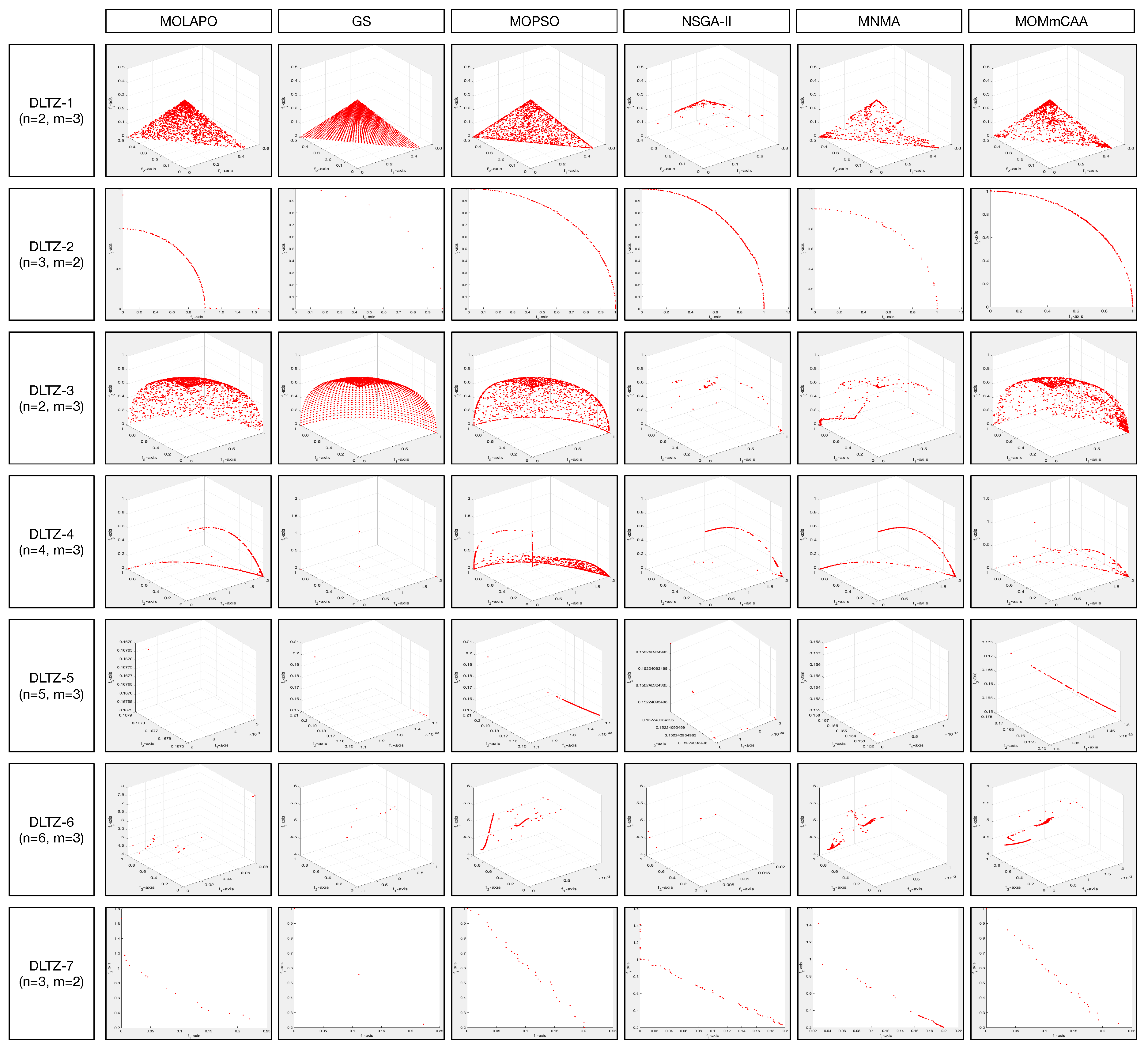
values than MOLAPO, GS, MOPSO, NSGA-II, and MNMA for 6, 4, 1, 7, and 5 out of the 7 instances, respectively. Overall, the EI statistics are similar to those for HV. Figure 4 plots the representative PFs obtained by six comparison MOEAs. In summary, MOMmCAA has a competitive performance on the DLTZ benchmark.

4.3. Quadratic Instances

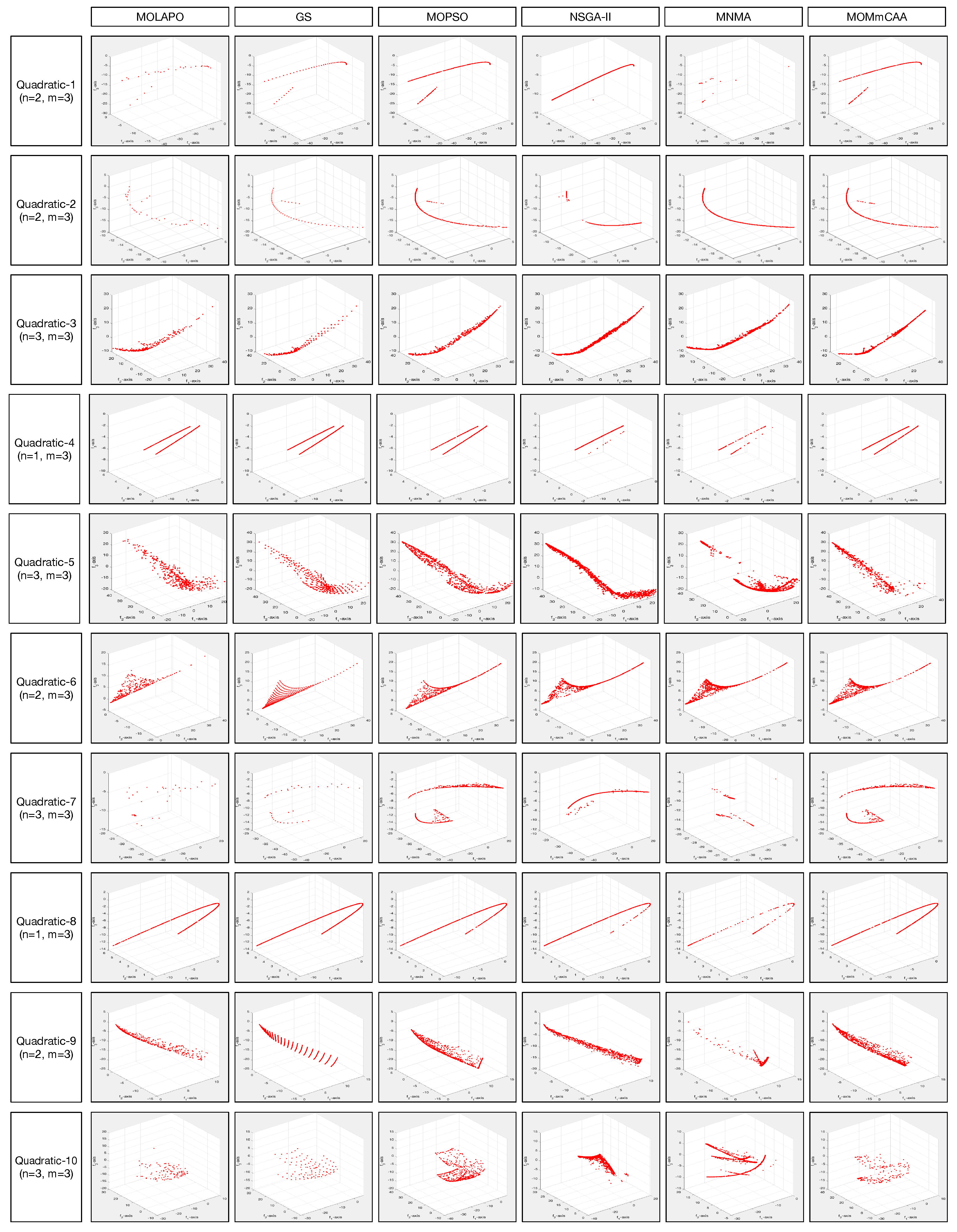
The Quadratics test set is a randomly generated test set described in [46]. The objective functions are all of the form

\frac{1}{2} x^{T} A x + b x + c

where the components of A, b, and c are random numbers in the range

[- 1, 1]

. A is not a symmetric matrix; the test set is non-convex. Table 5, Table 6 and Table 7 expose the results of the metric values obtained by algorithms over 10 quadratic problems.

Table 5 displays that MOMmCAA obtains significantly better

H V

values than MOLAPO, GS, MOPSO, NSGA-II, and MNMA for 6, 7, 2, 8, and 7 out of the 8 instances, respectively. Regarding the overall mean rankings, MOMmCAA obtained the second optimal mean rank value, below MOPSO, and followed by the other algorithms. MOMmCAA has a performance that is significantly equivalent to the other three instances concerning MOPSO. Table 6 presents that MOMmCAA achieves 10, 10, 5, 8, and 7 better C metric values than MOLAPO, GS, MOPSO, NSGA-II, and MNMA, respectively. This indicates the quality of the solutions obtained by the MOMmCAA. Table 7 depicts the overall performance of six algorithms for the EI metric values. MOMmCAA yields significantly better

E I

values than MOLAPO, GS, MOPSO, NSGA-II, and MNMA for 9, 7, 6, 8, and 9 out of the 10 instances, respectively. Figure 5 shows the representative Pareto fronts (PFs) obtained by six comparison MOEAs. In summary, MOMmCAA has a competitive performance on the Quadratic benchmark.

4.4. CEC2020 Instances

Table 8, Table 9 and Table 10 present the results of the metric values obtained by algorithms over 10 benchmark CEC2020 problems.

Table 8 depicts that MOMmCAA obtains significantly better

H V

values than MOLAPO, GS, MOPSO, NSGA-II, and MNMA for 8, 9, 4, 8, and 7 out of the 10 instances, respectively. In the case of MOPSO, there are 6 results with no significant difference. Concerning the overall mean rankings, MOMmCAA obtains the optimal mean rank value. MOMmCAA has a bad performance on MMF-2 and MMF-7 test instances. In summary, MOMmCAA is superior to all the other MOEAs on this metric. Table 9 shows that MOMmCAA achieves 10, 10, 7, 8, and 6 better C metric values than MOLAPO, GS, MOPSO, NSGA-II, and MNMA, respectively. In the case of MNMA, there are 4 results with the worst significant difference. Table 10 summarizes the overall performance of six algorithms in terms of EI metric values. MOMmCAA yields significantly better

E I

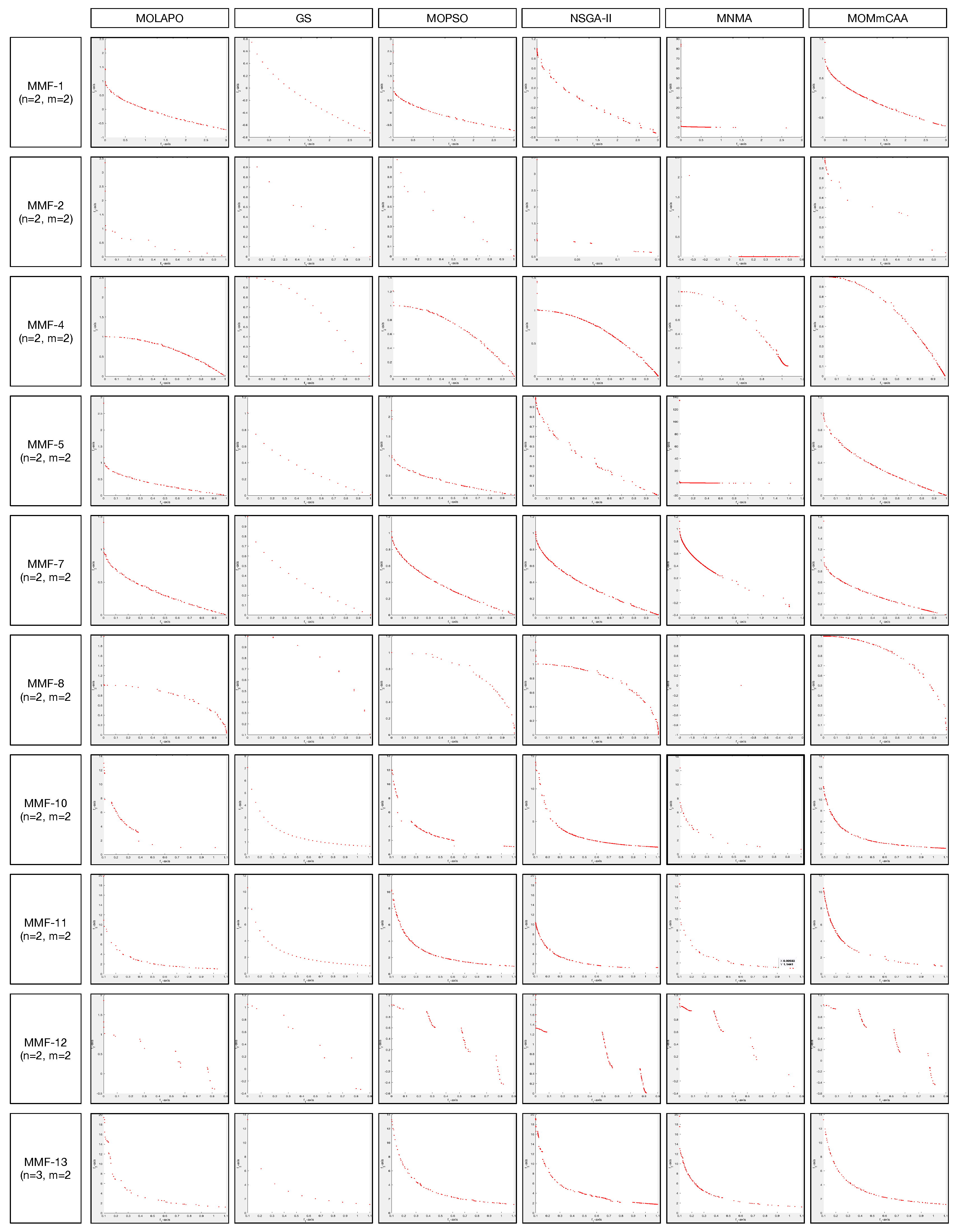
values than MOLAPO, GS, MOPSO, NSGA-II, and MNMA for 10, 10, 6, 10, and 8 out of the 10 instances, respectively. Figure 6 depicts the representative Pareto fronts (PFs) obtained by seven comparison MOEAs. In summary, MOMmCAA has a competitive behavior on the CEC2020 benchmark.

5. Engineering Design Problems

In this section, the capability of the MOMmCAA is evaluated in solving two real-world engineering design problems: the four-bar truss design and the disk brake design.

5.1. Four-Bar Truss Design Problem

In the four-bar truss design [54], structural volume

h_{1}

and displacement

h_{2}

have to be minimized. This problem consists of four design variables

z_{1}

z_{4}

corresponding to the cross-sectional area of parts 1 to 4, as illustrated in Figure 7 The equations are given below:

\begin{matrix} Minimize : \\ h_{1} (z) = 200 (2 z_{1} + \sqrt{2 z_{2}} + \sqrt{z_{3}} + z_{4}) \\ h_{2} (z) = 0.01 (\frac{2}{z_{1}} + \frac{2 \sqrt{2}}{z_{2}} - \frac{2 \sqrt{2}}{z_{3}} + \frac{2}{z_{4}}) \\ where : \\ 1 \leq z_{1} \leq 3, 1.4142 \leq z_{2} \leq 3 \\ 1.4142 \leq z_{3} \leq 3, 1 \leq z_{4} \leq 3 \end{matrix}

(6)

5.2. Disk Brake Design Problem

The multiobjective disc brake design problem is proposed in [55] with five constraints and two objectives to be minimized, namely the stopping time

h_{1}

and brake mass

h_{2}

. This problem has four design variables: the inner radius of the disc

z_{1}

, the outer radius

z_{2}

, engaging force

z_{3}

, and the number of friction surfaces

z_{4}

. Figure depicts the system, and Eq. 7 describes the problem.

\begin{matrix} Minimize : \\ h_{1} (z) = (4.9 * 10^{- 5}) (z_{2}^{2} - z_{1}^{2}) (z_{4} - 1) \\ h_{2} (z) = (9.82 * 10^{6}) \frac{z_{2}^{2} - z_{1}^{2}}{(z_{2}^{3} - z_{1}^{3}) (z_{4} z_{3})} \\ Subject to : \\ g_{1} (z) = z_{2} - z_{1} - 20 \\ g_{2} (z) = 30 - (2.5 (z_{4} - 1)) \\ g_{3} (z) = 0.4 - \frac{z_{3}}{3.14 * (z_{2}^{2} - z_{1}^{2})} \\ g_{4} (z) = 1 - (2.22 * 10^{-} 3) \frac{z_{3} (z_{2}^{3} - z_{1}^{3})}{{(z_{2}^{2} - z_{1}^{2})}^{2}} \\ g_{5} (z) = (2.66 * 10^{- 2}) \frac{z_{3} z_{4} (z_{2}^{3} - z_{1}^{3})}{(z_{2}^{2} - z_{1}^{2})} - 900 \\ where : \\ 55 \leq z_{1} \leq 80, 75 \leq z_{2} \leq 110 \\ 1000 \leq z_{3} \leq 3000, 2 \leq z_{4} \leq 20 \end{matrix}

(7)

5.3. Results of Design Problem

Table 11 presents the statistical results of MOMmCAA and the other algorithms in dealing with the engineering design problems using performance metrics

H V

, C and

E I

. It can be seen that MOMmCAA is one of the two best algorithms for these metrics in these cases, showing the competitiveness of the algorithm. MOMmCAA can calculate better results than MOLAPO, GS, NSGA-II, and MNMA, and MOMmCAA’s results are very close to MOPSO’s. Figure 9 presents the obtaind PFs for the two engineering design problems.

6. Conclusions and Further Work

This paper presents a new multiobjective optimization algorithm called MOMmCAA, inspired by the neighborhood and local interaction rules of majority and minority cellular automata. The randomness, concurrency, and information exchange between the smart-cells generated by applying the different rules produce an appropriate balance between exploration and exploitation actions.

Comparative computational testing was done with 27 test functions with various characteristics such as a convex, concave, mixed, disconnected, or degenerated PF that challenged the MOMmCAA and were compared against other 5 algorithms recognized for their efficiency. The experiments showed satisfactory performance of MOMmCAA.

Engineering multiobjective problems used in recent literature were also taken to test MOMmCAA against results obtained by other methods. MOMmCAA also demonstrated its high quality in finding solutions to these problems, proving, in general, its competitiveness against other recent metaheuristics.

In future work, it is proposed to use other strategies for handling PF solutions, such as applying a niche strategy. Another possibility is to continue modifying metaheuristic algorithms based on cellular automata to deal with multiobjective problems.

Author Contributions

Conceptualization, J.C.S.-T.-M. and J.M.-M.; methodology, J.C.S.-T.-M. and U.A.H.-U.; validation, J.C.S.-T.-M. and J.M.-M.; formal analysis, J.C.S.-T.-M., L.L.-M. and N.H.-R.; investigation, J.C.S.-T.-M., U.A.H.-U., and J.M.-M.; resources, N.H.-R. and L.L.-M.; writing—original draft preparation, J.C.S.-T.-M., U.A.H.-U., and J.M.-M.; writing—review and editing, N.H.-R. and L.L.-M.; visualization, J.C.S.-T.-M. and N.H.-R.; supervision, J.M.-M. and L.L.-M.; funding acquisition, J.C.S.-T.-M. All authors have read and agreed to the published version of the manuscript.

Funding

This study was supported by the Autonomous University of Hidalgo (UAEH) and the National Council for Humanities, Science and Technology (CONAHCYT) with project number F003-320109.

Institutional Review Board Statement

Not applicable.

Informed Consent Statement

Not applicable.

Data Availability Statement

The MOMmCAA source code is available on Github https://github.com/juanseck/MOMmCAA (accessed on 23 August 2024).

Conflicts of Interest

The authors declare that they have no known competing financial interest or personal relationships that could have appeared to influence the work reported in this paper.

References

Zhou, A.; Qu, B.Y.; Li, H.; Zhao, S.Z.; Suganthan, P.N.; Zhang, Q. Multiobjective evolutionary algorithms: A survey of the state of the art. Swarm and evolutionary computation 2011, 1, 32–49. [CrossRef]
Holland, J.H. Genetic algorithms. Scientific american 1992, 267, 66–73. [CrossRef]
Eberhart, R.; Kennedy, J. Particle swarm optimization. Proceedings of the IEEE international conference on neural networks. Citeseer, 1995, Vol. 4, pp. 1942–1948.
Dorigo, M.; Birattari, M.; Stutzle, T. Ant colony optimization. IEEE computational intelligence magazine 2006, 1, 28–39. [CrossRef]
Van Laarhoven, P.J.; Aarts, E.H.; van Laarhoven, P.J.; Aarts, E.H. Simulated annealing; Springer, 1987.
Deb, K.; Pratap, A.; Agarwal, S.; Meyarivan, T. A fast and elitist multiobjective genetic algorithm: NSGA-II. IEEE transactions on evolutionary computation 2002, 6, 182–197. [CrossRef]
Zhang, Q.; Li, H. MOEA/D: A Multiobjective Evolutionary Algorithm Based on Decomposition. IEEE Transactions on Evolutionary Computation 2007, 11, 712–731. [CrossRef]
Zitzler, E.; Laumanns, M.; Thiele, L. SPEA2: Improving the strength Pareto evolutionary algorithm. TIK report 2001, 103.
Coello, C.C.; Lechuga, M.S. MOPSO: A proposal for multiple objective particle swarm optimization. Proceedings of the 2002 Congress on Evolutionary Computation. CEC’02 (Cat. No. 02TH8600). IEEE, 2002, Vol. 2, pp. 1051–1056.
Alaya, I.; Solnon, C.; Ghedira, K. Ant colony optimization for multi-objective optimization problems. 19th IEEE international conference on tools with artificial intelligence (ICTAI 2007). IEEE, 2007, Vol. 1, pp. 450–457.
Chen, Z.G.; Zhan, Z.H.; Lin, Y.; Gong, Y.J.; Gu, T.L.; Zhao, F.; Yuan, H.Q.; Chen, X.; Li, Q.; Zhang, J. Multiobjective cloud workflow scheduling: A multiple populations ant colony system approach. IEEE transactions on cybernetics 2018, 49, 2912–2926. [CrossRef]
Zhou, S.Z.; Zhan, Z.H.; Chen, Z.G.; Kwong, S.; Zhang, J. A multi-objective ant colony system algorithm for airline crew rostering problem with fairness and satisfaction. IEEE Transactions on Intelligent Transportation Systems 2020, 22, 6784–6798. [CrossRef]
Zhang, X.; Zhan, Z.H.; Fang, W.; Qian, P.; Zhang, J. Multipopulation ant colony system with knowledge-based local searches for multiobjective supply chain configuration. IEEE Transactions on Evolutionary Computation 2021, 26, 512–526. [CrossRef]
Smith, K.I.; Everson, R.M.; Fieldsend, J.E. Dominance measures for multi-objective simulated annealing. Proceedings of the 2004 congress on evolutionary computation (IEEE Cat. No. 04TH8753). IEEE, 2004, Vol. 1, pp. 23–30.
Mirjalili, S.; Jangir, P.; Saremi, S. Multi-objective ant lion optimizer: a multi-objective optimization algorithm for solving engineering problems. Applied Intelligence 2017, 46, 79–95. [CrossRef]
Mirjalili, S.; Jangir, P.; Mirjalili, S.Z.; Saremi, S.; Trivedi, I.N. Optimization of problems with multiple objectives using the multi-verse optimization algorithm. Knowledge-Based Systems 2017, 134, 50–71. [CrossRef]
Mirjalili, S.; Gandomi, A.H.; Mirjalili, S.Z.; Saremi, S.; Faris, H.; Mirjalili, S.M. Salp Swarm Algorithm: A bio-inspired optimizer for engineering design problems. Advances in engineering software 2017, 114, 163–191. [CrossRef]
Zhan, Z.H.; Li, J.; Cao, J.; Zhang, J.; Chung, H.S.H.; Shi, Y.H. Multiple populations for multiple objectives: A coevolutionary technique for solving multiobjective optimization problems. IEEE transactions on cybernetics 2013, 43, 445–463. [CrossRef]
Liu, S.C.; Chen, Z.G.; Zhan, Z.H.; Jeon, S.W.; Kwong, S.; Zhang, J. Many-objective job-shop scheduling: A multiple populations for multiple objectives-based genetic algorithm approach. IEEE Transactions on Cybernetics 2021, 53, 1460–1474. [CrossRef]
Tejani, G.G.; Kumar, S.; Gandomi, A.H. Multi-objective heat transfer search algorithm for truss optimization. Engineering with Computers 2021, 37, 641–662. [CrossRef]
Tejani, G.G.; Pholdee, N.; Bureerat, S.; Prayogo, D. Multiobjective adaptive symbiotic organisms search for truss optimization problems. Knowledge-based systems 2018, 161, 398–414. [CrossRef]
Kumar, S.; Tejani, G.G.; Pholdee, N.; Bureerat, S.; Jangir, P. Multi-objective teaching-learning-based optimization for structure optimization. Smart Science 2022, 10, 56–67. [CrossRef]
Khodadadi, N.; Talatahari, S.; Dadras Eslamlou, A. MOTEO: a novel multi-objective thermal exchange optimization algorithm for engineering problems. Soft Computing 2022, 26, 6659–6684. [CrossRef]
Kumar, S.; Jangir, P.; Tejani, G.G.; Premkumar, M.; Alhelou, H.H. MOPGO: A new physics-based multi-objective plasma generation optimizer for solving structural optimization problems. IEEE Access 2021, 9, 84982–85016. [CrossRef]
Khodadadi, N.; Azizi, M.; Talatahari, S.; Sareh, P. Multi-objective crystal structure algorithm (MOCryStAl): introduction and performance evaluation. IEEE Access 2021, 9, 117795–117812. [CrossRef]
Nouri-Moghaddam, B.; Ghazanfari, M.; Fathian, M. A novel multi-objective forest optimization algorithm for wrapper feature selection. Expert Systems with Applications 2021, 175, 114737. [CrossRef]
Yüzgeç, U.; Kusoglu, M. Multi-objective harris hawks optimizer for multiobjective optimization problems. BSEU Journal of Engineering Research and Technology 2020, 1, 31–41.
Abdel-Basset, M.; Mohamed, R.; Mirjalili, S.; Chakrabortty, R.K.; Ryan, M. An efficient marine predators algorithm for solving multi-objective optimization problems: analysis and validations. IEEE Access 2021, 9, 42817–42844. [CrossRef]
Tawhid, M.A.; Savsani, V. Multi-objective sine-cosine algorithm (MO-SCA) for multi-objective engineering design problems. Neural Computing and Applications 2019, 31, 915–929. [CrossRef]
Azizi, M.; Talatahari, S.; Khodadadi, N.; Sareh, P. Multiobjective atomic orbital search (MOAOS) for global and engineering design optimization. IEEE Access 2022, 10, 67727–67746. [CrossRef]
Sabarinath, P.; Thansekhar, M.; Saravanan, R. Multiobjective optimization method based on adaptive parameter harmony search algorithm. Journal of Applied Mathematics 2015, 2015, 165601. [CrossRef]
Got, A.; Moussaoui, A.; Zouache, D. A guided population archive whale optimization algorithm for solving multiobjective optimization problems. Expert Systems with Applications 2020, 141, 112972. [CrossRef]
Pathak, S.; Mani, A.; Sharma, M.; Chatterjee, A. Decomposition Based Quantum Inspired Salp Swarm Algorithm for Multiobjective Optimization. IEEE Access 2022, 10, 105421–105436. [CrossRef]
Shi, Y.; Liu, H.; Gao, L.; Zhang, G. Cellular particle swarm optimization. Information Sciences 2011, 181, 4460–4493. [CrossRef]
Lopes, R.A.; de Freitas, A.R. Island-cellular model differential evolution for large-scale global optimization. Proceedings of the Genetic and Evolutionary Computation Conference Companion, 2017, pp. 1841–1848.
Seck-Tuoh-Mora, J.C.; Hernandez-Romero, N.; Lagos-Eulogio, P.; Medina-Marin, J.; Zuñiga-Peña, N.S. A continuous-state cellular automata algorithm for global optimization. Expert Systems with Applications 2021, 177, 114930. [CrossRef]
Vafashoar, R.; Morshedlou, H.; Rezvanian, A.; Meybodi, M.R.; Vafashoar, R.; Morshedlou, H.; Rezvanian, A.; Meybodi, M.R. Applications of cellular learning automata and reinforcement learning in global optimization. Cellular Learning Automata: Theory and Applications 2021, pp. 157–224.
Seck-Tuoh-Mora, J.C.; Lopez-Arias, O.; Hernandez-Romero, N.; Martínez, G.J.; Volpi-Leon, V. A New Algorithm Inspired on Reversible Elementary Cellular Automata for Global Optimization. IEEE Access 2022, 10, 112211–112229. [CrossRef]
Zhu, G.; Ma, L. Cellular ant algorithm for multi-objective function optimization. Control and Decision 2007, 22, 1317.
Sidiropoulos, E. Multi-objective cellular automata optimization. Cellular Automata: 10th International Conference on Cellular Automata for Research and Industry, ACRI 2012, Santorini Island, Greece, September 24-27, 2012. Proceedings 10. Springer, 2012, pp. 131–140.
Zhu, D.; Zhan, T.; Zhang, Y.; Tian, H. Algorithm and application of cellular multi-objective particle swarm optimization. Transactions of the Chinese Society for Agricultural Machinery 2013, 44, 280–287.
Birashk, A.; Kordestani, J.K.; Meybodi, M.R. Cellular teaching-learning-based optimization approach for dynamic multi-objective problems. Knowledge-Based Systems 2018, 141, 148–177. [CrossRef]
Seck-Tuoh-Mora, J.C.; Hernandez-Romero, N.; Santander-Baños, F.; Volpi-Leon, V.; Medina-Marin, J.; Lagos-Eulogio, P. A majority–minority cellular automata algorithm for global optimization. Expert Systems with Applications 2022, 203, 117379. [CrossRef]
Nematollahi, A.F.; Rahiminejad, A.; Vahidi, B. A novel multi-objective optimization algorithm based on Lightning Attachment Procedure Optimization algorithm. Applied Soft Computing 2019, 75, 404–427. [CrossRef]
Kokkolaras, M. C. Audet and W. Hare: Derivative-free and blackbox optimization. Springer series in operations research and financial engineering: 2017, 302 pp, DOI 10.1007/978-3-319-68913-5, 2019.
Nadeau, P.C. Multiobjective Nelder-Mead algorithm using a mesh-map of weighted sums. PhD thesis, University of British Columbia, 2020.
Zenil, H.; Martinez, G.J. Cellular automata. Scholarpedia 2024, 19, 53227. [CrossRef]
Clarke, K.C. Cellular automata and agent-based models. In Handbook of regional science; Springer, 2021; pp. 1751–1766.
Knowles, J.D.; Corne, D.W. Approximating the nondominated front using the Pareto archived evolution strategy. Evolutionary computation 2000, 8, 149–172. [CrossRef]
Coello, C.A.C.; Pulido, G.T.; Lechuga, M.S. Handling multiple objectives with particle swarm optimization. IEEE Transactions on evolutionary computation 2004, 8, 256–279. [CrossRef]
Ulrich, T.; Bader, J.; Zitzler, E. Integrating decision space diversity into hypervolume-based multiobjective search. Proceedings of the 12th annual conference on Genetic and evolutionary computation, 2010, pp. 455–462.
Bandyopadhyay, S.; Pal, S.K.; Aruna, B. Multiobjective GAs, quantitative indices, and pattern classification. IEEE Transactions on Systems, Man, and Cybernetics, Part B (Cybernetics) 2004, 34, 2088–2099. [CrossRef]
Zitzler, E.; Thiele, L.; Laumanns, M.; Fonseca, C.M.; Da Fonseca, V.G. Performance assessment of multiobjective optimizers: An analysis and review. IEEE Transactions on evolutionary computation 2003, 7, 117–132. [CrossRef]
Cheng, F.; Li, X. Generalized center method for multiobjective engineering optimization. Engineering Optimization 1999, 31, 641–661. [CrossRef]
Ray, T.; Liew, K.M. Society and civilization: an optimization algorithm based on the simulation of social behavior. IEEE Transactions on Evolutionary Computation 2003, 7, 386–396. [CrossRef]

Figure 1. Examples of cellular automata with 2 states and neighborhood size 3 applying majority, minority and majority with probability evolution rules.

Figure 2. Majority-minority Cellular Automata Algorithm (MmCAA).

Figure 3. PS repository management using PF hypercubes.

Figure 4. The representative PFs obtained by seven MOEAs on DLTZ benchmark.

Figure 5. The representative PFs obtained by six MOEAs on Quadratic benchmark set.

Figure 6. The representative PFs obtained by six MOEAs on CEC2020 benchmark set.

Figure 7. Description of the four-bar truss design problem.

Figure 8. Description of the disk brake design problem.

Figure 9. The representative PFs obtained by sixs MOEAs on two engineering design problems.

Table 1. Parameters of the algorithms (MOLAPO, GS, MOPSO, NSGA-II, MNMA, and MOMmCAA) used for comparison.

Algorithm	Parameters
MOLAPO	$F E = 2$ , $c a p = 50$
GS	$n u m p a r t s = 20$ , $c a p = 50$
MOPSO	$C 1 = C 2 = 2$ , $w = w m a x - t \times (w m a x - w m i n) / (t m a x)$ ,
	$w m a x = 0.9$ , $w m i n = 0.4$ , $c a p = 50$
NSGA-II	$p c r o s s = 0.7$ , $n c r o s s = 2 * r o u n d (p c r o s s * 100 / 2)$ , $p m u t = 0.4$ ,
	$n m u t = r o u n d (p m u t * 100)$ , $m u = 0.02$ , $S i g m a = 0.1 * (v m a x - v m i n)$
MNMA	$δ^{e} = 2$ , $δ^{o c} = 0.5$ , $δ^{i c} = - 0.5$ , $γ = 5$
MOMmCAA	$c a p = 50$ , $n_{S} = 11$ , $n_{n e} = 3$ , $n_{i n t} = 5$ , $p r o p = 5$ , $2 \leq n_{r} \leq 5$

Table 2. Statistics (mean(std. dev.)) of Hypervolume metric values of final populations obtained by MOLAPO, GS, MOPSO, NSGA-II, MNMA, and MOMmCAA algorithms over 30 independent runs on DLTZ benchmark.

Fn	MOLAPO	GS	MOPSO	NSGA-II	MNMA	MOMmCAA
DLTZ1	0.99429(0.00194)[3]+	0.99994(0.00352)[1]+	0.99625(0.01576)[2]+	0.80818(0.03725)[5]-	0.95796(0.01212)[6]-	0.98678(0.00284)[4]
DLTZ2	0.99609(0.00399)[4]≈	0.97096(0.00267)[6]-	0.99853(0.00162)[1]+	0.99693(0.00309)[2]≈	0.98508(0.00572)[5]-	0.99691(0.00333)[3]
DLTZ3	0.99053(0.00459)[3]+	0.99899(0.00228)[1]+	0.99738(0.00322)[2]+	0.63267(0.05291)[6]-	0.70551(0.06081)[5]-	0.97466(0.00583)[4]
DLTZ4	0.81151(0.04801)[3]-	0.15972(0.00396)[6]-	0.99165(0.03466)[1]+	0.67624(0.17103)[4]-	0.64341(0.17161)[5]-	0.89404(0.05888)[2]
DLTZ5	0.07332(0.02604)[6]-	0.34796(0.01714)[3]-	0.94131(0.05117)[2]-	0.17332(0.02604)[4]-	0.11067(0.00561)[5]-	0.99498(0.01031)[1]
DLTZ6	0.99003(0.00255)[5]-	0.99731(0.00081)[3]≈	0.99977(0.00058)[1]≈	0.9799(0.00573)[6]-	0.99441(0.01468)[4]-	0.99843(0.00084)[2]
DLTZ7	0.87676(0.03064)[5]-	0.84891(0.06436)[6]-	0.98959(0.00744)[2]≈	0.98982(0.00082)[1]≈	0.93897(0.09525)[4]-	0.98946(0.03301)[3]
Mean rank	4.14	3.71	1.57	4.00	4.85	2.71
$+ / - / \approx$	2/4/1	2/4/1	4/1/2	0/5/2	0/7/0	—

Table 3. Statistics (mean(std. dev.)) of Contribution metric values of final populations obtained by MOLAPO, GS, MOPSO, NSGA-II, MNMA, and MOMmCAA algorithms over 30 independent runs on DLTZ benchmark.

Fn	MOLAPO	GS	MOPSO	NGSGA-II	MNMA	MOMmCAA
DLTZ1	0.81513(2.5e-16)[2]-	0.79783(1.8e-16)[5]-	0.81411(2.6e-16)[3]-	0.80951(0.01246)[4]-	0.5406(0.00605)[6]-	0.99994(1.5e-16)[1]
DLTZ2	0.60881(0.04617)[5]-	0.76008(0.06445)[3]-	0.99082(0.04048)[1]+	0.64211(0.16553)[4]-	0.19691(0.03617)[6]-	0.92488(0.01163)[2]
DLTZ3	0.81521(6.8e-17)[2]-	0.79783(2.5e-16)[5]-	0.81411(6.8e-17)[3]-	0.81208(0.00876)[4]-	0.46125(0.03017)[6]-	0.99761(2.3e-17)[1]
DLTZ4	0.81011(6.9e-17)[3]-	0.79783(1.5e-16)[5]-	0.81411(6.9e-17)[2]-	0.80433(7.9e-17)[4]-	0.66554(0.06417)[6]-	0.96642(1.9e-17)[1]
DLTZ5	0.00106(0.00561)[6]-	0.14161(0.01798)[4]-	0.89958(0.11419)[2]-	0.16198(0.25733)[3]-	0.00703(0.00259)[5]-	0.91351(0.12699)[1]
DLTZ6	0.07939(0.00016)[6]-	0.12859(0.00108)[5]-	0.35269(0.01687)[3]-	0.97912(0.00036)[1]+	0.29689(0.09089)[4]-	0.52038(0.01358)[2]
DLTZ7	0.14766(0.00345)[5]-	0.09762(0.02054)[6]-	0.76907(0.01705)[3]-	0.77836(0.03273)[2]-	0.76552(0.06844)[4]-	0.94891(0.00012)[1]
Mean rank	4.14	4.71	2.42	3.14	5.28	1.28
$+ / - / \approx$	0/7/0	0/7/0	1/6/0	1/6/0	0/7/0	—

Table 4. Statistics (mean(std. dev.)) of Epsilon Indicator metric values of final populations obtained by MOLAPO, GS, MOPSO, NSGA-II, MNMA, and MOMmCAA algorithms over 30 independent runs on DLTZ benchmark.

Fn	MOLAPO	GS	MOPSO	NGSGA-II	MNMA	MOMmCAA
DLTZ1	0.99251(0.00643)[3]≈	0.99636(0.00328)[2]+	0.99946(0.00151)[1]+	0.87914(0.03957)[6]-	0.96551(0.01401)[5]-	0.99242(0.00535)[4]
DLTZ2	0.99369(0.00604)[3]-	0.97315(0.00895)[6]-	0.99851(0.00151)[1]≈	0.99316(0.00704)[4]-	0.98192(0.12301)[5]-	0.99849(0.00592)[2]
DLTZ3	0.95559(0.02415)[4]-	0.97026(0.02491)[2]+	0.99957(0.00205)[1]+	0.69537(0.07809)[6]-	0.77792(0.09631)[5]-	0.96893(0.02171)[3]
DLTZ4	0.80537(0.11288)[4]-	0.90474(0.02358)[2]+	0.99786(0.00692)[1]+	0.75078(0.15433)[5]-	0.73808(0.15012)[6]-	0.84343(0.11741)[3]
DLTZ5	0.87907(0.00867)[5]-	0.73707(2.9e-10)[6]-	0.91127(3.3e-10)[4]-	0.97907(8.6e-10)[2]-	0.92175(3.4e-10)[3]-	0.99983(4.9e-11)[1]
DLTZ6	0.89671(0.05005)[5]-	0.92768(0.00218)[4]-	0.99916(0.00022)[1]+	0.44597(0.13399)[6]-	0.96871(0.06117)[2]≈	0.96843(0.02285)[3]
DLTZ7	0.89964(0.03153)[6]-	0.94273(0.00382)[5]-	0.99577(0.00727)[1]+	0.94297(0.09443)[4]-	0.96892(0.01423)[3]≈	0.96945(0.01462)[2]
Mean rank	4.28	3.85	1.43	4.71	4.14	2.57
$+ / - / \approx$	0/6/1	3/4/0	5/1/1	0/7/0	0/5/2	—

Table 5. Statistics (mean(std. dev.)) of Hypervolume metric values of final populations obtained by MOLAPO, GS, MOPSO, NSGA-II, MNMA, and MOMmCAA algorithms over 30 independent runs on quadratic test suites.

Fn	MOLAPO	GS	MOPSO	NSGA-II	MNMA	MOMmCAA
Quad-1	0.78322(0.04654)[5]-	0.91926(0.23614)[3]-	0.99998(0.01051)[1]+	0.90089(0.03592)[4]-	0.75012(0.17974)[6]-	0.97308(0.01009)[2]
Quad-2	0.75569(0.03641)[6]-	0.78349(0.23614)[5]-	0.99422(0.09865)[1]+	0.82711(0.03899)[4]-	0.92676(0.15884)[3]-	0.96682(0.01187)[2]
Quad-3	0.98283(0.00386)[5]-	0.97448(0.00405)[6]-	0.99018(0.00341)[4]-	0.99833(0.00223)[1]+	0.99541(0.00414)[2]≈	0.99535(0.00505)[3]
Quad-4	0.99888(0.00171)[1]≈	0.99579(0.00463)[3]≈	0.99118(0.00323)[4]-	0.98363(0.00372)[5]-	0.97515(0.00481)[6]-	0.99691(0.00299)[2]
Quad-5	0.94097(0.01085)[4]≈	0.92327(0.01642)[5]-	0.99992(0.00444)[1]+	0.99325(0.00375)[2]+	0.89467(0.01418)[6]-	0.96875(0.00594)[3]
Quad-6	0.98348(0.00502)[4]≈	0.96742(0.00823)[6]-	0.98765(0.00721)[3]≈	0.97599(0.01148)[5]-	0.99932(0.00151)[1]≈	0.99652(0.00389)[2]
Quad-7	0.43281(0.20744)[6]-	0.46508(0.08089)[5]-	0.98807(0.06536)[1]+	0.78886(0.05951)[3]-	0.56825(0.18535)[4]-	0.93741(0.01437)[2]
Quad-8	0.99299(0.00428)[4]≈	0.99837(0.00282)[1]≈	0.99306(0.00418)[3]≈	0.96498(0.01516)[5]-	0.96222(0.02049)[6]-	0.99478(0.00586)[2]
Quad-9	0.96921(0.00929)[4]-	0.97883(0.00618)[3]-	0.99772(0.00109)[1]≈	0.90104(0.02035)[6]-	0.90771(0.02575)[5]-	0.99738(0.00583)[2]
Quad-10	0.86775(0.01173)[4]-	0.97449(0.00462)[2]+	0.98141(0.00552)[1]+	0.73001(0.06776)[6]-	0.84311(0.05941)[5]-	0.92103(0.01019)[3]
Mean rank	4.30	3.90	2.00	4.10	4.40	2.30
$+ / - / \approx$	0/6/4	1/7/2	5/2/3	2/8/0	0/8/2	—

Table 6. Statistics (mean(std. dev.)) of Contribution metric values of final populations obtained by MOLAPO, GS, MOPSO, NSGA-II, MNMA, and MOMmCAA algorithms over 30 independent runs on quadratic test suites.

Fn	MOLAPO	GS	MOPSO	NGSGA-II	MNMA	MOMmCAA
Quad-1	0.75487(0.02278)[4]-	0.85594(0.32768)[3]-	0.99384(0.02372)[1]+	0.65634(0.07167)[5]-	0.63046(0.07081)[6]-	0.91587(0.06981)[2]
Quad-2	0.61502(0.01407)[6]-	0.76286(0.16743)[4]-	0.91895(0.19035)[1]≈	0.75641(0.29032)[5]-	0.82091(0.01546)[3]-	0.91815(0.14073)[2]
Quad-3	0.58342(0.01813)[5]-	0.57459(0.01185)[6]-	0.65944(0.03274)[4]-	0.98271(0.08238)[1]+	0.85912(0.13298)[2]+	0.74987(0.03573)[3]
Quad-4	0.95912(0.13298)[2]-	0.94987(0.03573)[3]-	0.85944(0.02274)[4]-	0.67459(0.08185)[6]-	0.68342(0.01813)[5]-	0.98271(0.08238)[1]
Quad-5	0.84931(0.04191)[4]-	0.66213(0.02118)[5]-	0.98481(0.04525)[1]+	0.93985(0.14828)[2]+	0.63827(0.01627)[6]-	0.88621(0.07419)[3]
Quad-6	0.82908(0.04868)[3]-	0.66273(0.02023)[6]-	0.70668(0.04084)[4]-	0.66434(0.01723)[5]-	0.99658(0.01309)[1]+	0.91766(0.07619)[2]
Quad-7	0.52661(0.05169)[5]-	0.46672(0.08213)[6]-	0.97117(0.04531)[1]+	0.84717(0.21804)[3]-	0.74241(0.01537)[4]-	0.92648(0.03031)[2]
Quad-8	0.77726(0.00723)[4]-	0.88706(0.00482)[2]-	0.80734(0.00928)[3]-	0.60466(0.01226)[5]-	0.57185(0.01626)[6]-	0.99518(0.00316)[1]
Quad-9	0.54521(0.02159)[5]-	0.43691(0.01182)[6]-	0.87067(0.04239)[2]-	0.68009(0.07186)[4]-	0.85437(0.08877)[3]-	0.99906(0.00512)[1]
Quad-10	0.61702(0.00557)[6]-	0.66071(0.01124)[5]-	0.90513(0.08038)[2]+	0.75366(0.16515)[4]-	0.97229(0.06946)[1]+	0.05858(0.80182)[3]
Mean rank	4.40	4.60	2.30	4.00	3.70	2.00
$+ / - / \approx$	0/10/0	0/10/0	4/5/1	2/8/0	3/7/0	—

Table 7. Statistics (mean(std. dev.)) of Epsilon Indicator metric values of final populations obtained by MOLAPO, GS, MOPSO, NSGA-II, MNMA, and MOMmCAA algorithms over 30 independent runs on quadratic test suites.

Fn	MOLAPO	GS	MOPSO	NGSGA-II	MNMA	MOMmCAA
Quad-1	0.62402(0.09443)[5]-	0.77487(0.12757)[3]-	0.99517(0.00447)[2]≈	0.69627(0.33691)[4]-	0.50285(0.27533)[6]-	0.99818(0.00367)[1]
Quad-2	0.54496(0.09916)[6]-	0.80271(0.26354)[3]-	0.98797(0.02443)[1]+	0.55422(0.28261)[5]-	0.59969(0.11613)[4]-	0.97799(0.01943)[2]
Quad-3	0.86202(0.17741)[5]-	0.79807(0.11866)[6]-	0.87514(0.18563)[4]-	0.97767(0.03478)[1]+	0.91085(0.14061)[3]-	0.94322(0.06748)[2]
Quad-4	0.97834(0.03436)[1]+	0.91831(0.13431)[3]-	0.77563(0.18626)[4]-	0.39845(0.11916)[6]-	0.46857(0.16193)[5]-	0.94391(0.06796)[2]
Quad-5	0.88448(0.10603)[4]-	0.41847(0.04586)[6]-	0.99095(0.01752)[1]+	0.90822(0.06635)[3]-	0.49757(0.05502)[5]-	0.93836(0.07011)[2]
Quad-6	0.65502(0.11956)[6]-	0.70243(0.13052)[5]-	0.73762(0.10192)[4]-	0.88065(0.05199)[3]≈	0.96589(0.04309)[1]+	0.89991(0.07718)[2]
Quad-7	0.55817(0.03239)[5]-	0.53664(0.11288)[6]-	0.95711(0.12275)[2]-	0.77369(0.11982)[3]-	0.63564(0.15328)[4]-	0.97471(0.02668)[1]
Quad-8	0.92344(0.08841)[3]-	0.98789(0.05241)[1]+	0.91887(0.01305)[4]-	0.81193(0.04545)[6]-	0.89861(0.05604)[5]-	0.94885(0.04763)[2]
Quad-9	0.65007(0.15543)[6]-	0.96713(0.11283)[1]+	0.95369(0.02206)[2]≈	0.71652(0.13191)[5]-	0.72003(0.20242)[4]-	0.94849(0.11392)[3]
Quad-10	0.67132(0.07651)[4]-	0.99714(0.01208)[1]+	0.91749(0.09838)[2]+	0.51204(0.02972)[6]-	0.57531(0.08959)[5]-	0.79207(0.02124)[3]
Mean rank	4.50	3.50	2.60	4.20	4.20	2.00
$+ / - / \approx$	1/9/0	3/7/0	2/6/2	1/8/1	1/9/0	—

Table 8. Statistics (mean(std. dev.)) of Hypervolume metric values of final populations obtained by MOLAPO, GS, MOPSO, NSGA-II, MNMA, and MOMmCAA algorithms over 30 independent runs on CEC2020 test suites.

Fn	MOLAPO	GS	MOPSO	NGSGA-II	MNMA	MOMmCAA
MMF-1	0.99551(0.00380)[2]≈	0.97921(0.00435)[5]-	0.99521(0.00364)[3]≈	0.98501(0.01006)[4]-	0.95330(0.04687)[6]-	0.99979(0.00064)[1]
MMF-2	0.94519(0.21376)[3]≈	0.94513(0.21394)[5]≈	0.94531(0.21341)[2]≈	0.94461(0.21545)[6]-	0.97327(0.20311)[1]+	0.94516(0.21382)[4]
MMF-4	0.92765(0.36793)[3]-	0.91716(0.36644)[4]-	0.89891(0.36922)[5]-	0.83784(0.36838)[6]-	0.97852(0.24517)[2]-	0.99834(0.36891)[1]
MMF-5	0.99061(0.00888)[4]-	0.98516(0.00726)[6]-	0.99182(0.00773)[3]-	0.98652(0.01121)[5]-	0.99627(0.00481)[2]≈	0.99764(0.00421)[1]
MMF-7	0.97362(0.04312)[5]-	0.96621(0.03988)[6]-	0.97559(0.04193)[2]≈	0.97549(0.04257)[4]≈	0.99685(0.04818)[1]+	0.97551(0.04175)[3]
MMF-8	0.91162(0.06317)[4]-	0.91027(0.05915)[5]-	0.95558(0.05191)[2]-	0.93241(0.05217)[3]-	0.39131(0.05318)[6]-	0.97133(0.04661)[1]
MMF-10	0.86078(0.00265)[6]-	0.93318(0.04895)[4]-	0.96027(0.02389)[3]-	0.97936(0.00291)[1]≈	0.90559(0.09678)[5]-	0.97213(0.02239)[2]
MMF-11	0.85121(0.03382)[6]-	0.86273(0.00116)[5]-	0.97232(0.02115)[1]≈	0.92785(0.08872)[3]-	0.88915(0.02615)[4]-	0.97159(0.00188)[2]
MMF-12	0.96184(0.00387)[5]-	0.93192(0.08422)[6]-	0.99736(0.00341)[2]≈	0.96397(0.01387)[4]-	0.97736(0.00942)[3]-	0.99878(0.00297)[1]
MMF-13	0.90689(0.00547)[6]-	0.91923(0.00261)[5]-	0.99918(0.00171)[1]≈	0.97883(0.00491)[3]-	0.96891(0.02477)[4]-	0.99823(0.00201)[2]
Mean rank	4.4	5.1	2.4	3.9	3.2	1.8
$+ / - / \approx$	0/8/2	0/9/1	0/4/6	0/8/2	2/7/1	—

Table 9. Statistics (mean(std. dev.)) of Contribution metric values of final populations obtained by MOLAPO, GS, MOPSO, NSGA-II, MNMA, and MOMmCAA algorithms over 30 independent runs on CEC2020 test suites.

Fn	MOLAPO	GS	MOPSO	NGSGA-II	MNMA	MOMmCAA
MMF-1	0.21284(0.02899)[6]-	0.48681(0.06161)[3]-	0.26768(0.03194)[5]-	0.31514(0.06624)[4]-	0.97631(0.04619)[1]+	0.87346(0.13758)[2]
MMF-2	0.27155(0.00148)[6]-	0.32403(0.01227)[4]-	0.35886(0.08701)[3]-	0.80862(0.00594)[5]-	0.99938(0.15996)[1]+	0.93693(0.12977)[2]
MMF-4	0.13284(0.05839)[6]-	0.54038(0.24031)[3]-	0.22977(0.11048)[5]-	0.32635(0.14577)[4]-	0.84895(0.21811)[2]-	0.87174(0.28415)[1]
MMF-5	0.19131(0.01754)[6]-	0.39972(0.05242)[3]-	0.23097(0.03746)[5]-	0.35141(0.05769)[4]-	0.99779(0.00745)[1]+	0.94446(0.01699)[2]
MMF-7	0.17123(0.28283)[6]-	0.77256(0.09347)[3]-	0.36233(0.06165)[5]-	0.61661(0.21303)[4]-	0.98383(0.14643)[1]+	0.90298(0.14448)[2]
MMF-8	0.37523(0.00382)[5]-	0.87316(0.00935)[3]-	0.86239(0.00617)[4]-	0.91538(0.00281)[1]+	0.17183(0.00146)[6]-	0.90118(0.00144)[2]
MMF-10	0.87312(0.04205)[6]-	0.90113(0.02852)[4]-	0.93021(0.01318)[3]-	0.95619(0.00239)[2]≈	0.89254(0.03678)[5]-	0.95732(0.00197)[1]
MMF-11	0.67961(0.04162)[6]-	0.77343(0.01834)[5]-	0.94072(0.02231)[1]+	0.91676(0.00719)[3]-	0.79925(0.03318)[4]-	0.93662(0.01129)[2]
MMF-12	0.51512(0.07343)[5]-	0.49052(0.02043)[6]-	0.98542(0.06019)[2]≈	0.61316(0.16228)[3]-	0.59515(0.28308)[4]-	0.98662(0.05113)[1]
MMF-13	0.50813(0.08822)[6]-	0.61112(0.06131)[5]-	0.96189(0.08838)[1]+	0.80553(0.07759)[4]-	0.83055(0.07981)[3]-	0.91891(0.06131)[2]
Mean rank	5.8	3.9	3.4	3.4	2.8	1.7
$+ / - / \approx$	0/10/0	0/10/0	2/7/1	1/8/1	4/6/0	—

Table 10. Statistics (mean(std. dev.)) of Epsilon Indicator metric values of final populations obtained by MOLAPO, GS, MOPSO, NSGA-II, MNMA, and MOMmCAA algorithms over 30 independent runs on CEC2020 test suites.

Fn	MOLAPO	GS	MOPSO	NGSGA-II	MNMA	MOMmCAA
MMF-1	0.97871(0.04936)[3]-	0.95288(0.04101)[4]-	0.98026(0.04723)[2]≈	0.93496(0.04759)[5]-	0.83513(0.10702)[6]-	0.98328(0.04980)[1]
MMF-2	0.95869(0.02934)[3]-	0.93286(0.02099)[4]-	0.96028(0.02721)[2]≈	0.91494(0.02757)[5]-	0.76529(0.12365)[6]-	0.96327(0.02981)[1]
MMF-4	0.65857(0.03934)[6]-	0.83867(0.02297)[3]-	0.66026(0.02828)[5]≈	0.71492(0.02958)[4]-	0.84026(0.10361)[2]-	0.86325(0.01979)[1]
MMF-5	0.88703(0.12261)[4]-	0.87936(0.11639)[5]-	0.89222(0.12298)[3]-	0.87874(0.12048)[6]-	0.98581(0.02851)[1]≈	0.98511(0.01242)[2]
MMF-7	0.82891(0.13589)[6]-	0.83145(0.13391)[4]-	0.83452(0.13742)[3]-	0.83102(0.13476)[5]-	0.99888(0.04667)[1]+	0.93331(0.01372)[2]
MMF-8	0.77395(0.00437)[5]-	0.79002(0.00392)[4]-	0.89991(0.00026)[1]≈	0.86967(0.00381)[3]-	0.31309(0.03895)[6]-	0.89949(0.00102)[2]
MMF-10	0.86115(0.00415)[6]-	0.89181(0.00811)[5]-	0.91921(0.01139)[4]≈	0.93512(0.00667)[2]-	0.93021(0.00231)[3]-	0.94163(0.00319)[1]
MMF-11	0.69518(0.01644)[6]-	0.79594(0.02179)[5]-	0.90235(0.00861)[1]+	0.83652(0.00437)[3]-	0.80525(0.00659)[4]-	0.89742(0.00193)[2]
MMF-12	0.74875(0.20031)[6]-	0.91482(0.01096)[5]-	0.98928(0.01135)[2]≈	0.92809(0.09053)[4]-	0.95293(0.03567)[3]-	0.99569(0.01255)[1]
MMF-13	0.93695(0.01154)[5]-	0.86241(0.11932)[6]-	0.99654(0.01017)[1]+	0.94589(0.03174)[4]-	0.95759(0.02445)[3]-	0.97549(0.03012)[2]
Mean rank	4.8	4.5	2.4	4.1	3.5	1.5
$+ / - / \approx$	0/10/0	0/10/0	2/6/2	0/10/0	1/8/1	—

Table 11. Statistics (mean(std. dev.)) of all metric values of final populations obtained by MOLAPO, GS, MOPSO, NSGA-II, MNMA, and MOMmCAA algorithms over 30 independent runs on Four-Bar Truss and Disk Brake design problems.

Four-Bar Truss	MOLAPO	GS	MOPSO	NGSGA-II	MNMA	MOMmCAA
HV	0.84592(0.01231)[6]	0.87194(0.02341)[5]	0.95983(0.00419)[2]	0.93705(0.00987)[3]	0.91821(0.03775)[4]	0.96785(0.00262)[1]
C	0.26667(0.01461)[6]	0.39275(0.07258)[5]	0.97902(0.07049)[1]	0.77658(0.30337)[3]	0.74773(0.02033)[4]	0.96819(0.06412)[2]
EI	0.51275(0.06052)[6]	0.58243(0.02745)[5]	0.92044(0.03891)[1]	0.89137(0.20592)[3]	0.86035(0.23895)[4]	0.91848(0.02702)[2]
Disk Brake	MOLAPO	GS	MOPSO	NGSGA-II	MNMA	MOMmCAA
HV	0.87805(0.01808)[5]	0.87372(0.00512)[6]	0.99473(0.00245)[1]	0.98576(0.00236)[4]	0.99232(0.00278)[3]	0.99319(0.00127)[2]
C-7	0.64986(0.08828)[5]	0.53468(0.13525)[6]	0.91281(0.22025)[2]	0.82961(0.24068)[3]	0.78477(0.37482)[4]	0.91281(0.22025)[1]
EI	0.76378(0.06086)[5]	0.73299(0.02521)[6]	0.96142(0.00923)[2]	0.92163(0.03259)[3]	0.89365(0.08881)[4]	0.99714(0.00809)[1]

Disclaimer/Publisher’s Note: The statements, opinions and data contained in all publications are solely those of the individual author(s) and contributor(s) and not of MDPI and/or the editor(s). MDPI and/or the editor(s) disclaim responsibility for any injury to people or property resulting from any ideas, methods, instructions or products referred to in the content.

© 2024 by the authors. Licensee MDPI, Basel, Switzerland. This article is an open access article distributed under the terms and conditions of the Creative Commons Attribution (CC BY) license (http://creativecommons.org/licenses/by/4.0/).

Copyright: This open access article is published under a Creative Commons CC BY 4.0 license, which permit the free download, distribution, and reuse, provided that the author and preprint are cited in any reuse.

MDPI Initiatives

Important Links

Choose an area of interest and we will send you notifications of new preprints at your preferred frequency.

Disclaimer

Multiobjective Majority-minority Cellular Automata Algorithm (MOMmCAA) for Global and Engineering Design Optimization

Abstract

1. Introduction

2. The Proposed Multiobjective Majority-minority Cellular Automata Algorithm (MOMmCAA)

3. Basic Concepts of Cellular Automata with Majority Rule

3.1. Multiobjective Majority-minority Cellular Automata Algorithm (MOMmCAA)

4. Computational Experiments to Compare MOMmCAA with Other Algorithms

4.1. Benchmark Instances

4.2. DLTZ Instances

4.3. Quadratic Instances

4.4. CEC2020 Instances

5. Engineering Design Problems

5.1. Four-Bar Truss Design Problem

5.2. Disk Brake Design Problem

5.3. Results of Design Problem

6. Conclusions and Further Work

Author Contributions

Funding

Institutional Review Board Statement

Informed Consent Statement

Data Availability Statement

Conflicts of Interest

References

MDPI Initiatives

Important Links

Subscribe