1. Introduction
Japan's urban landscape, characterized by rapid urbanization and cutting-edge technological advances, is at the forefront of addressing complex challenges in the construction and infrastructure sectors. However, in Japan, the significant structural damage of-ten caused by the settlement or tilting of structures, due to the liquefaction of saturated sandy soils during large earthquakes [
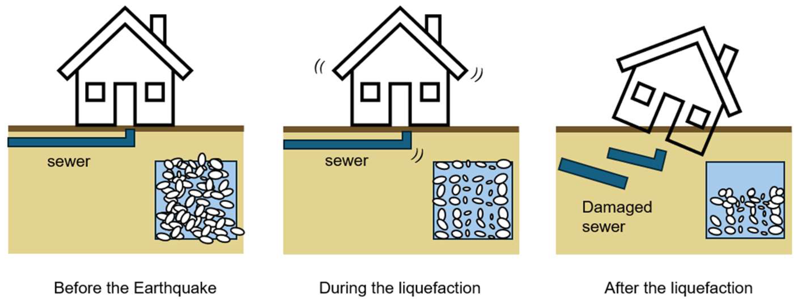
1]. As shown in
Figure 1, liquefaction is a phenomenon in which, when an earthquake occurs and the ground receives a strong shock, soil particles that were previously in contact and supporting each other break apart, and the entire ground becomes a viscous liquid-like state. When liquefaction occurs, water gushes out of the ground, and the previously stable ground suddenly becomes soft, causing buildings that were standing on it to sink (tilt), manholes and buried pipes to float, and the entire ground to flow downward. Liquefaction has become an important topic of geo technical engineering since the 1960s and significant efforts have been made on the assessment of liquefaction resistance of in situ soils. The current methodology for this assessment commonly relies on in situ measurements such as SPT-N (number of blows for 30-cm penetration in standard penetration tests; [
2,
3]). Case histories indicate that most of the damaging liquefaction disasters occurred in geologically very young, sandy deposits, such as those found in manmade islands, former river channels, filled lakes, swamps and so on [
4,
5], as well as pipeline backfill [
6]. The sudden instability of the ground during such events can lead to the catastrophic destruction of buildings and infrastructures, resulting in significant economic losses as well as the tragic loss of human life. This critical was further highlighted in [
1,
7,
8].
In order to promote the investigation and publish relevant results, deepen the public's awareness of the hazards of liquefaction, and do a good job in the prevention and control of liquefaction of residential land. The importance of smart cities is self-evident. Smart cities refer to the use of various information technologies or innovative ideas to integrate the constituent systems and services of the city in order to improve the efficiency of resource utilization, optimize urban management and services, and improve the quality of life of citizens. Specifically, the concept of "intelligence" is to enable humans to manage the state of production and life in a more sophisticated and dynamic way through the application of new generation information technology. The emergence of the Internet of Things makes it possible to access remote sensor data and to control the physical world from a distance, meaning that cities can effectively sense and manage essential elements such as the water supply, building operations, and road and transport networks [
9]. Data vitalization proposes a new paradigm for large-scale dataset analysis and offers ubiquitous data support for top-level applications for smart cities [
10,
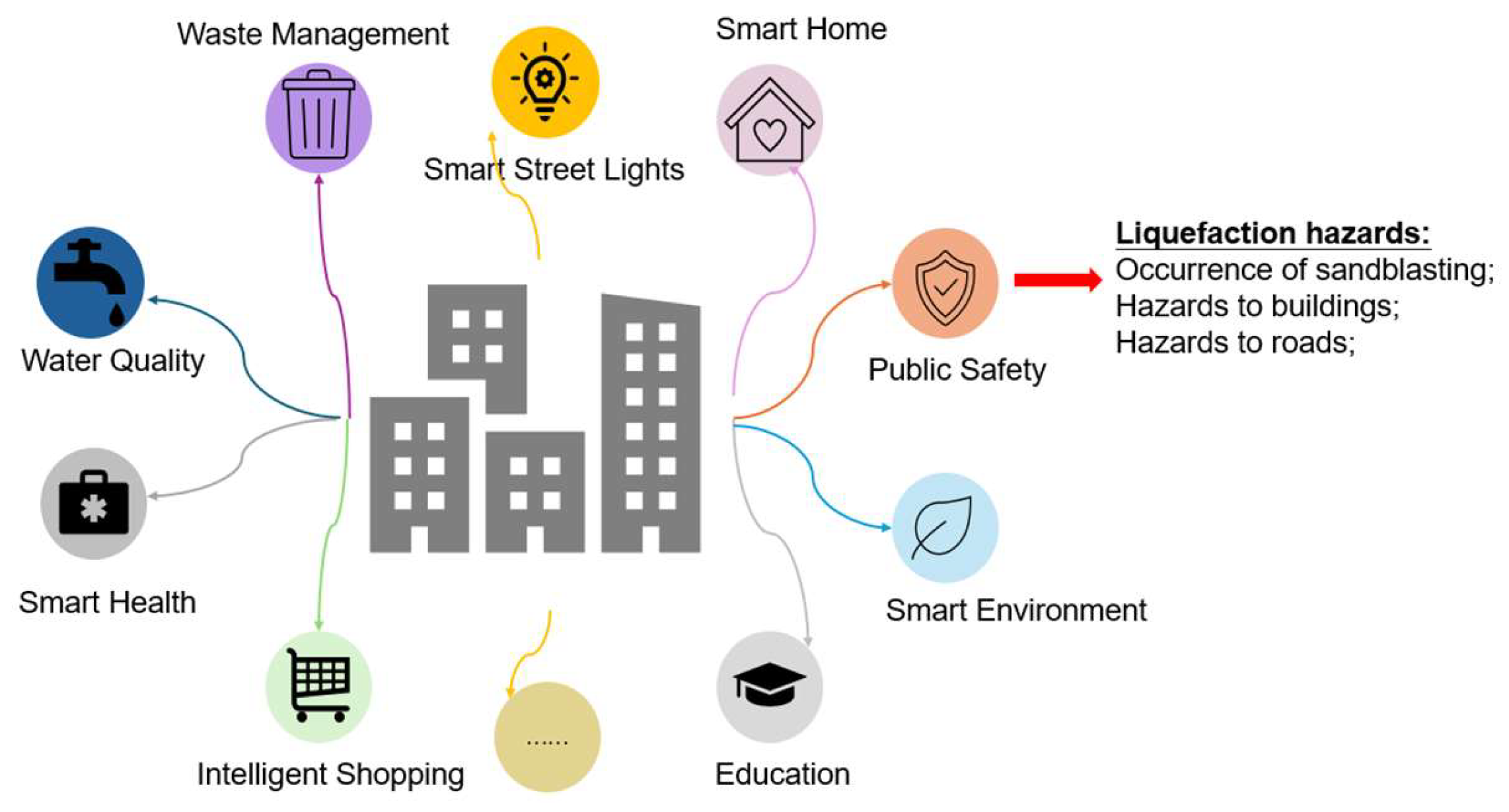
11]. For this study, as shown in
Figure 2, in the integration and visualization of the smart city, an AI-driven predictive model that synthesizes data from diverse databases, including geotechnical and geographic information, enhances urban resilience and promotes the development of a safer and more sustainable society. This approach contributes to the sustainable growth of smart cities and ensures the safety of their inhabitants [
12].
Nowadays, the monitoring technology for geology and liquefaction has been continuously improving, but it still has great limitations. The main reason is that traditional empirical methods lack credibility and universality. Therefore, the field of machine learning is expected to become a new field to improve the accuracy of prediction. Techniques such as artificial neural networks [
13], ensemble learning [
14,
15,
16,
17], which enhances prediction through algorithmic diversity, are at the forefront of spatial and temporal data analysis. At present, machine learning is widely used in many countries around the world for address prediction and other purposes [
18,
19]. By using machine learning to help better analyze geology and make predictions, it can help with city planning. This also reflects the widespread use and impact of machine learning around the world. The main purpose of this study is to use AI technology that goes beyond traditional technology to predict geological information, analyze reliable data sets, and create a new prediction model. Since this is a new field, this study is divided into creating a single model using neural networks and an integrated model that integrates multiple models using bagging for analysis and comparison. By comparing the results, a model with better prediction performance is obtained to solve Japan's liquefaction problem, hoping to obtain smart infrastructure and data-based smart cities. This also heralds a new era of urban development. By combining the ever-evolving new technologies with traditional research, we can help everyone better deal with urban development s and ensure a sustainable future.
2. About Artificial Neural Networks (ANNs)
A wide variety of models have been developed in the field of machine learning since the term "Machine Learning “was coined in1959 by ArthurSamuel [
20]. In many cases, they provide improved results [
21] due to their capacity for handling more complex data better than classical statistical methods [
22,
23]. Recent developments in computing technologies have produced several machine learning algorithms, especially Artificial Neural Networks (ANNs), which have the ability to operate nonlinearly [
24]. ANNs are a mathematical model or computational model that imitates the structure and function of biological neural networks and is used to estimate or approximate functions. ANNs have become popular and helpful model for classification, clustering, pattern recognition and prediction in many disciplines. ANNs are one type of model for machine learning (ML) and has become relatively competitive to conventional regression and statistical models regarding usefulness [
25]. The great potential of ANNs is the high-speed processing provided in a massive parallel implementation and this has heightened the need for research in this domain [
26,
27].
Regarding the creation of a PyTorch-based neural network model to predict the output, it is divided into the following 7 steps: defining the problem; preparing the dataset; defining the model; defining the loss function and optimizer; training the model; evaluating the model; and model tuning.
2.1. Defining the Problem
This study is to predict the bearing layer depth. The bearing layer is "a stratum that is sufficiently solid to bearing a particular building". In other words, it is "a stratum that is strong and does not easily undergo detrimental deformation when subjected to weight". A hammer weighing 63.5±0.5 kg is used to hit the drill rod at a free fall height of 76±1 cm to drive the sampler used in the standard penetration test into the ground 30 cm. The number of hits required is called the N-value. The N-value represents the relationship between soil moisture content and clay and organic matter content and is used to estimate the soil bearing load and the degree of settlement after drainage. N-value of 20 or less is often unstable as a foundation layer for civil engineering structures. In general, soil with an N-value of 20 or more or rock is desirable as a foundation bearing layer. When the N-value is between 30 and 50, it can be said that the layer is suitable as the foundation ground for civil engineering and building structures. If the N-value of 50 or more, it can be f the N-value of 50 or more, it can be judged to be very solid. It is a good bearing layer that can withstand even large structures such as high-rise condominiums [
28]. Therefore, in this study, the N-value is greater than 50 or more within the range of more than 3 m in a row, it is called the bearing layer [
29].
ML tools are aiming at solving two classic statistical tasks - classification (pattern recognition) and regression (function approximation) [
30]. The goal of the former is to predict real-valued labels for data, whilst the goal of the latter is to predict discrete labels [
31]. First, it needs to clarify whether the problem is regression or classification. Obviously, predicting bearing layer depth is a continuous value, so this is a regression problem.
2.2. Preparing the Dataset
This study used geological information survey data from Setegaya, Tokyo. The data came from the bearing layer depth and longitude and latitude of the actual survey conducted by the partner company. The corresponding elevatioN-values were found on the Tokyo Geographical Institute through the longitude and latitude. The specific data examples are shown in
Table 1. After collecting the data, we preprocessed the data, including processing missing values and outliers. For outliers in the data, choose to delete them directly; for missing values, since there are relatively few missing data, choose to complete the data using the mean. After confirming the relevance and feature importance, the data set was completed. A total of 433 data were used in this study. The data analysis of 433 data is shown in
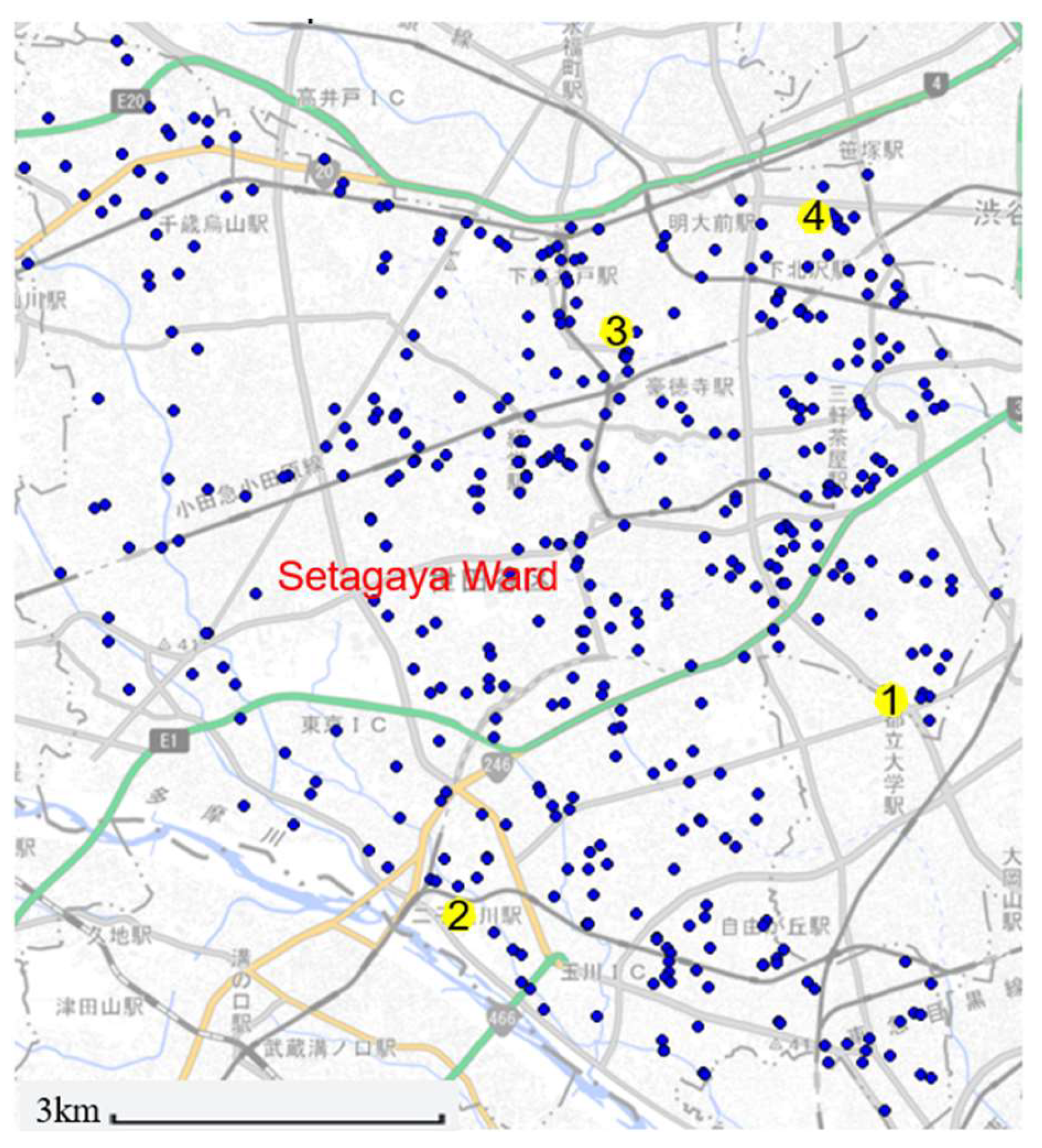
Table 2. Among the 433 data, the ratio of training set, verification set, and test set is: 7:2:1. In addition, the specific distribution of the 433 data on the map is shown in
Figure 3. The four locations listed in
Table 1 are also marked in
Figure 3.
2.3. Creating the Model
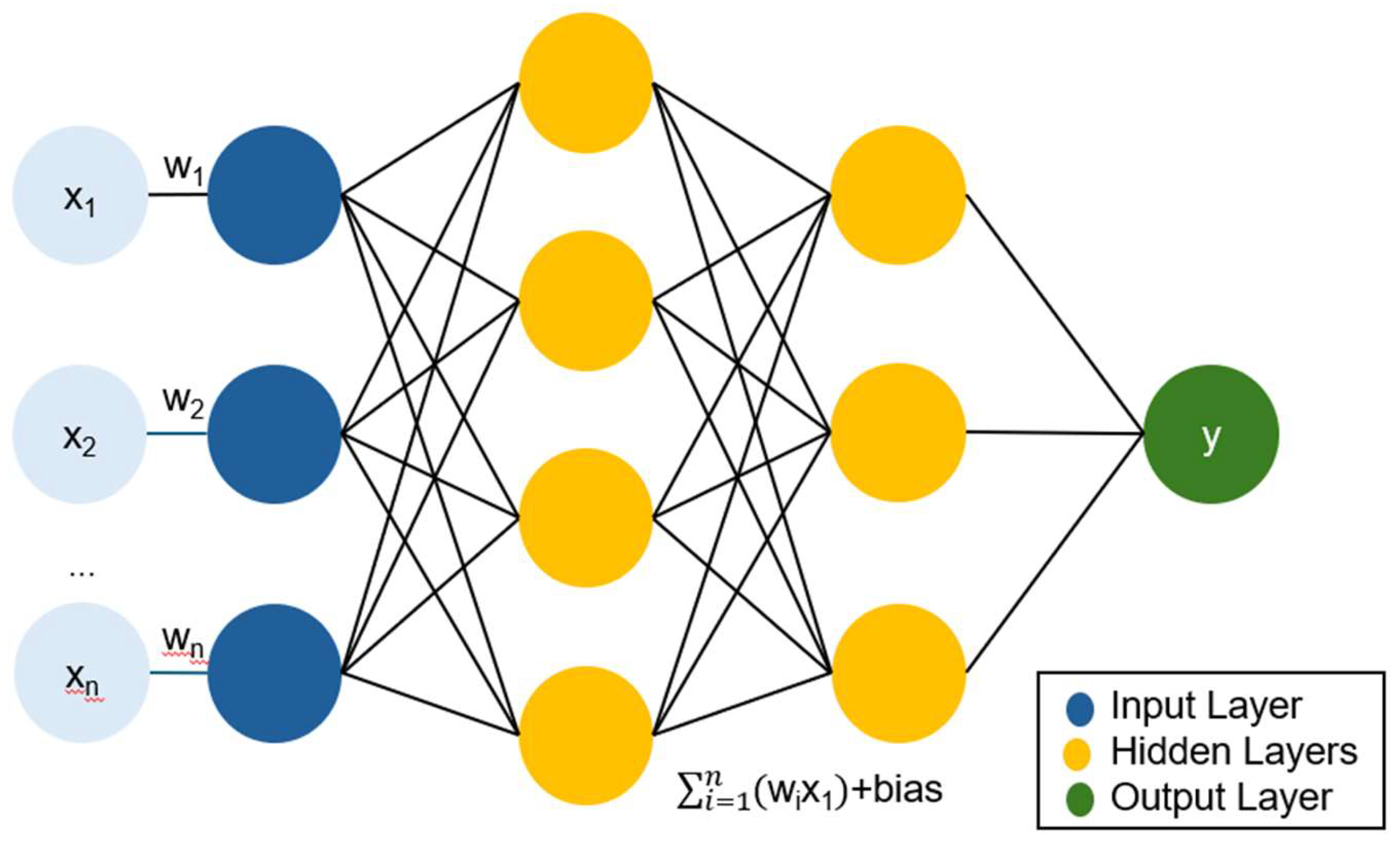
Use PyTorch to define a neural network model shown as
Figure 4. The activation function selects the most used ReLU in deep neural networks, and its calculation method is as follows Eq. (1).
When is less than 0, the output is 0, and when is greater than 0, the output is .
For a model with three inputs and one output, first define it as a simple fully connected network. Fully connected, in a neural network, means that every neuron in the current layer is directly connected to all neurons in the previous layer. This connection means that the output of the previous layer will be fully passed to every neuron in the current layer, and each neuron will perform a weighted summation of these inputs according to the weights and biases, and finally get the output through the activation function. For regression problems, the mean square error (MSE) is used as the loss function, and the optimizer selects the stochastic gradient descent (SGD). Regarding hyperparameter adjustment, manual adjustment is used.
3. Building the Bagging
Ensemble learning methods, which involve building and combining multiple learners, have been shown to produce better results and achieve improved generalisation compared with any of the constituent classifiers alone [
32,
33,
34]. Ensemble learning use multiple machine learning algorithms to produce weakly predictive results based on features extracted through a variety of projections on the data and fuse the results with various voting mechanisms to achieve a better performance than that obtained by any constituent algorithm alone [
35]. Many methods for constructing ensembles have been developed, but bagging, boosting and stacking are the commonly used techniques [
36]. Briefly, bagging (also known as bootstrap aggregation; [
37]) is the way to improve the stability and accuracy of MLA through training the same algorithm many times by using different subsets sampled from the training data [
38].
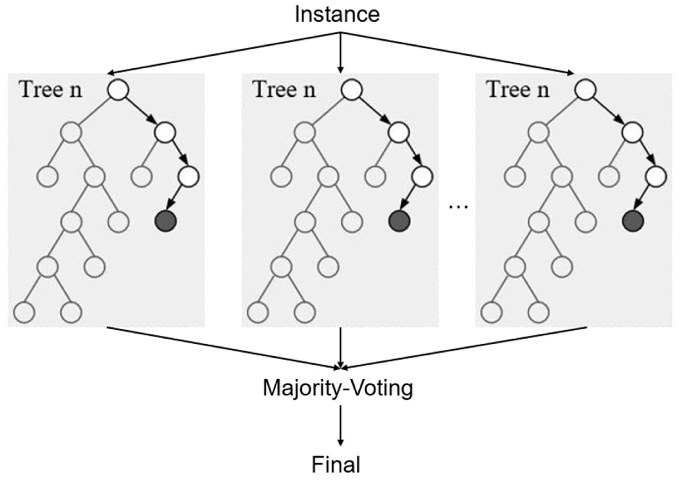
The aggregation of multiple learners leads to a lower variance of the model while its bias may remain the same given the bias-variance decomposition of error for machine learning models. Given multiple models of the same machine learning algorithm trained on different training data, the bias of the machine learning algorithm is the similarity between the models’ average prediction and the ground truth, and its variance is the difference between the predictions [
38]. Random forest [
39] as shown in
Figure 5 is a prominent implementation of bagging that uses decision trees and introduces additional features to the sampling process [
40].
After creating the model, hyperparameter tuning is still required. The optimization method selected is manual parameter tuning. Finally, it is confirmed that when the number of decision trees in the hyperparameter is 91, the model performance of the prediction model is the best. The specific hyperparameter values are shown in
Table 3. N_estimators is the number of sub-datasets generated by sampling the original data set with replacement, that is, the number of decision trees. Max_depth is the maximum depth of the decision tree. ‘None’ means that the decision tree will not limit the depth of the sub-tree when building the optimal model. Max_features is the maximum number of features considered when building the optimal model of the decision tree. ‘auto’ means that the maximum number of features is the square root of N. After creating the model, hyperparameter tuning is still required. The optimization method selected is manual parameter tuning. Finally, it is confirmed that when the number of decision trees in the hyperparameter is 91, the model performance of the prediction model is the best. The specific hyperparameter values are shown in
Table 3. The specific creation steps are to extract samples from the original data set using bootstrap sampling to form multiple sub-datasets. Secondly, for each sub-dataset, a decision tree is constructed. At each node, a part of the features is randomly selected for splitting. Next, the above steps are repeated until 91 decision trees are generated. Finally, 91 decision trees are cultivated using the sample data, and their predictions are averaged to derive the final prediction. This averaging process follows Eq. (2).
where
is the predicted value of the forest,
is the prediction of an individual decision tree, and
is the total number of decision trees.
4. Results and Discussion
In the context of smart city development, the integration of AI technology can significantly improve urban management. This study focuses on two case studies in Setagaya, Tokyo. The accuracy and effectiveness of these methods are critical for smart city applications, including urban planning, and environmental monitoring. Case-1 uses ANNs to create a prediction model and Case-2 uses bagging to create a prediction model, where the explanatory variables are latitude, longitude, elevation and bearing layer depth. The target variable is the bearing layer depth.
4.1. Results on Predicting Bearing Layer Depth
In the Case-1, the model created by ANNs was used to predict actual data of the bearing layer at 10 locations in Setegaya, Tokyo. The actual measurements at these locations provided the basis for evaluating the accuracy of the predictions, and the error values between the predicted and actual values were calculated.
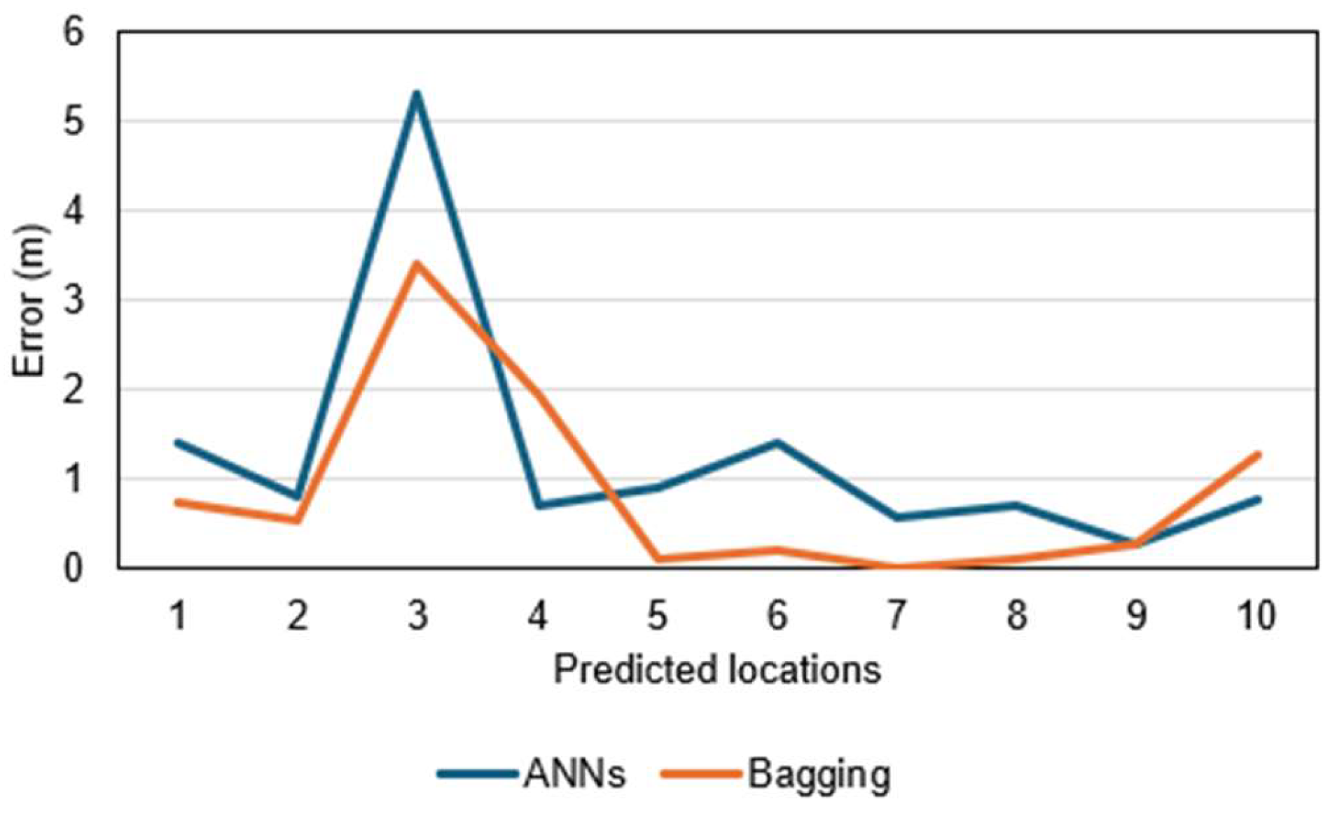
Table 4 and
Figure 6 give the specific prediction results and errors of 10 points in the two cases.
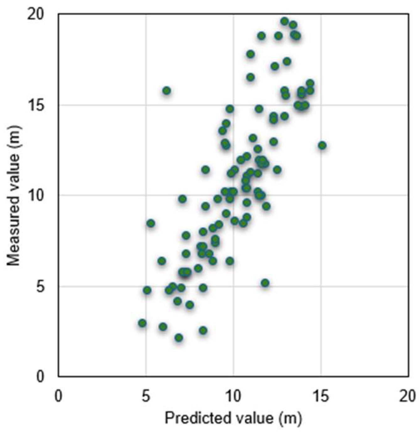
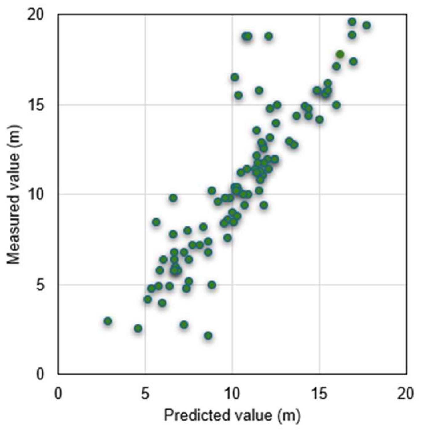
Figure 7 shows the results of all points in Case-1, indicating the accuracy of the method in spatial prediction. Like Case-1, Case-2 also used the same data and made predictions using the model created by bagging.
Figure 8 gives the prediction results of all points for Case-2.
4.2. Comparison of Prediction Results Between Neural Network and Bagging
Table 5 lists the prediction results of ANNs and bagging methods in detail, from which it can be seen that the prediction model of bagging method is better than ANNs in accuracy.
Table 5 uses four matrices of MAE, MSE, RMSE and confidence interval to evaluate the prediction accuracy of the models in Case-1 and Case-2. MAE is the mean of the absolute values of the errors; MSE is a measure of the mean squared error between the predicted and actual values in the dataset. The lower the MSE, the better the model fits the dataset. RMSE is a measure of the square root of the mean squared error between the predicted and actual values in the dataset. The lower the RMSE, the better the model fits the dataset. Based on these matrices, it can be concluded that the prediction model built using the bagging method is superior. The confidence interval (CI) can be regarded as an estimated range, which gives an interval that can be considered to contain an unknown population parameter at a certain confidence level. In other words, it is an estimate of the possible value of the population parameter, and this estimate is based on the data we obtained from the sample. Choose to set a 95% confidence level and a normal distribution, and finally calculate the confidence interval. The formula for the CI is shown as Eq. (3).
Among them, the critical value is 1.96.
This difference in performance motivates us to conduct a deeper analysis of the pros and cons of each method, especially in the context of their application in smart city planning and development.
It can be seen that compared with a single model; the prediction performance of the integrated model is improved by about 20%. Because a single model can only capture local features and patterns, it is easily affected by noise and randomness and may not perform well when facing complex tasks and large-scale data. However, ensemble learning can use the "wisdom" of multiple models to integrate the results of multiple models through voting, weighting, etc., which enhances the model's anti-noise ability and generalization ability. It can be concluded from many literatures [
41,
42]. Secondly, there are certain differences between individual learners, which will lead to different classification boundaries, that is, there may be errors. Then, after merging multiple individual learners, a more reasonable boundary can be obtained, the overall error rate can be reduced, and better results can be achieved. In the case where the data set is too small, you can perform partitioning and replacement operations separately to generate different data subsets, and then use the data subsets to train different learners, and finally merge them into a strong learner. Finally, because the data partition boundary is too complex, it is difficult to describe the situation using a linear model, so training multiple models and then fusing the models will achieve better model performance.
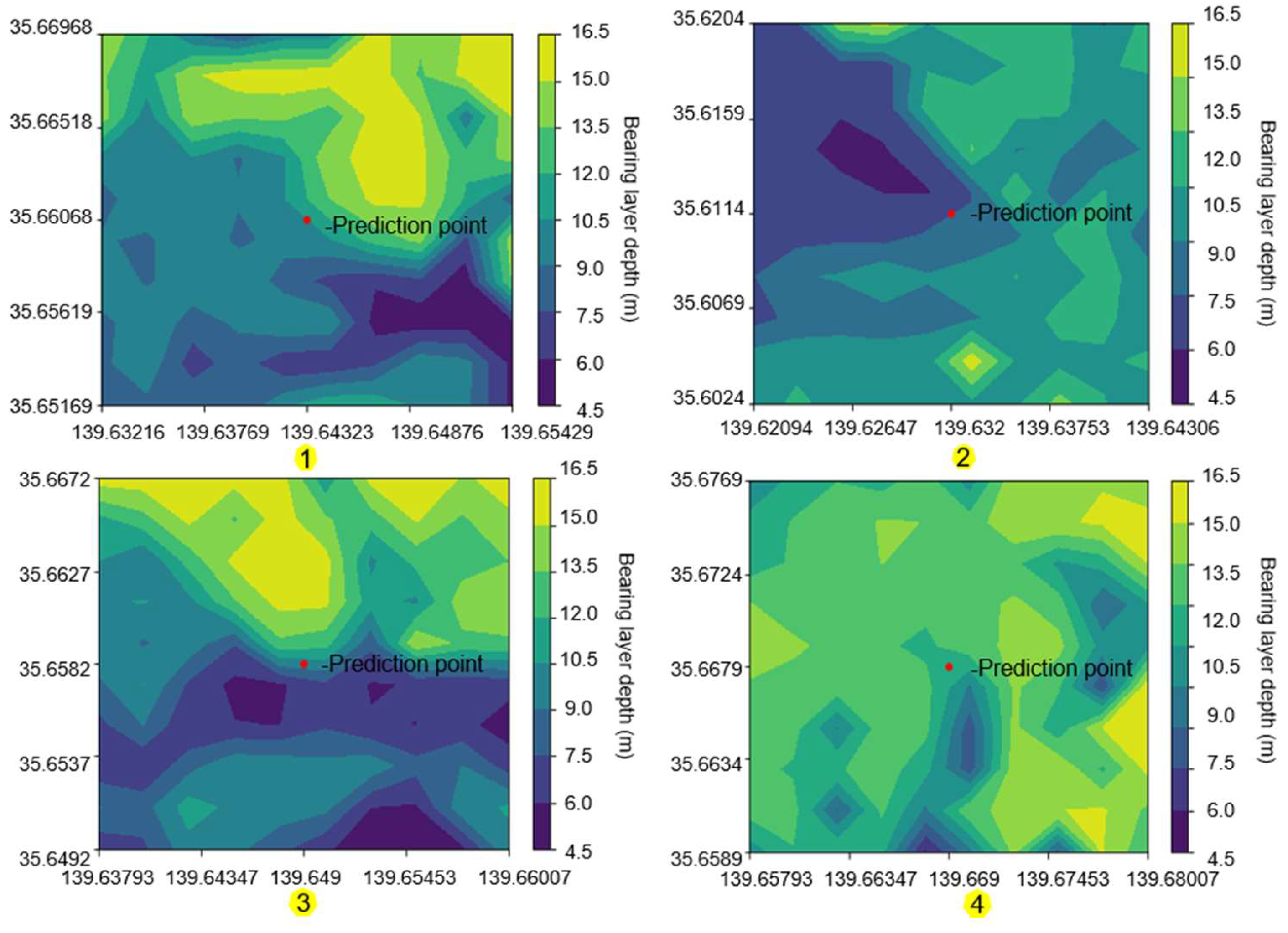
Improved the performance of the bagging model. Because of this, the depth of support for the observation points of the direct review, the addition of the bagging process, etc., and the high-level system. As shown in
Figure 9, divided
Figure 3 is an example of four points in the center, with a radius of 1km, and a contour map of the depth of support within the range.
In smart cities, bagging should help in the following aspects:
- (1)
Geological data analysis and prediction: Smart cities rely on a large amount of data for decision-making. Bagging can better analyze geological and other related data by reducing the variance of the model and improving the prediction performance.
- (2)
Hazard detection: In smart cities, it is very important to detect abnormal situations in a timely manner. The prediction model of the bearing layer depth created using bagging can be used as the basis for drawing disaster maps, so as to detect and respond to abnormal situations more effectively.
- (3)
Resource optimization: Based on the model of this study, it can help optimize resource allocation, such as setting a trusted bearing layer depth, predicting unknown points before construction, and omitting the geological survey step if it exceeds the trusted value, thereby reducing various costs.
These contents show the potential of bagging in smart cities, helping city managers make more informed decisions by improving data analysis and prediction performance.
5. Conclusions
At the heart of smart city development is the critical role of predictive analytics, which uses data to predict future scenarios and inform decision-making processes. This study establishes a high-precision prediction method for unknown points and unknown areas, demonstrating the great potential of machine learning in geotechnical engineering. The purpose of smart cities is to promote the optimal use of scarce resources and improve the quality of life of residents. Data collection technology is at the core of advancing smart city planning and achieving the desired results. Data-driven insights help local governments improve urban planning and urban service deployment, thereby improving the quality of life of residents. The potential of smart cities to use data for urban improvement is demonstrated. The specific results are as follows:
- (1)
By learning "latitude", "longitude", "altitude" and "bearing layer depth", high-precision bearing layer depth prediction is achieved. This accuracy is critical for smart cities because understanding the geotechnical properties of the ground can have a significant impact on infrastructure development from building construction to transportation network design.
- (2)
Compared with the prediction of a single model such as a neural network, the prediction performance of ensemble learning using bagging is better, and the prediction accuracy can be increased to about 20%. The use of bagging allows for better analysis of data, which can promote better urban planning.
- (3)
When using the multi-model ensemble learning method Bagging to predict geotechnical engineering survey results, it was found that a small change in the depth of the training data would have a significant impact on the model performance of the prediction model. This also emphasizes that the accuracy of the data must be guaranteed.
However, there are still major limitations to the current research results. First, the reliability of the prediction results cannot be determined. Because in today's research, the judgment of prediction performance is made by making predictions at the actual location that has been measured and comparing the predicted value with the actual value. But if a completely unknown point is predicted, how to ensure the credibility of the predicted point is a major that needs to be studied in the future. Secondly, the number of machine learning features is too small. The three feature quantities used today are not comprehensive enough for the depth of the bearing layer. Other relevant ground conditions will continue to be introduced in the future. Analyzing more features and ensuring their relevance will help further improve model performance. Finally, there are also many ways to learn ensembles, and how to choose the optimal solution is also a question to be considered in the future.
This study not only confirms the effectiveness of ensemble learning in the field of geological prediction, but also proves its potential in smart cities.
Author Contributions
Conceptualization, S.I.; methodology, S.I.; software, Y.C.; validation, S.I.; formal analysis, Y.C.; investigation, Y.C.; resources, S.I.; data curation, Y.C.; writing—original draft preparation, Y.C.; writing—review and editing, S.I.; visualization, S.I.; supervision, S.I.; project administration, S.I.; funding acquisition, S.I. All authors have read and agreed to the published version of the manuscript.
Funding
This research received no external funding.
Data Availability Statement
The data that support the findings of this study are available from the corresponding author, Shinya Inazumi, upon reasonable request.
Conflicts of Interest
The authors declare no conflicts of interest.
References
- Cong, Y.; Inazumi, S. Integration of smart city technologies with advanced predictive analytics for geotechnical investigations. Smart Cities 2024, 7, 3, 1089-1108. [CrossRef]
- Seed, H.B.; Idriss, I.M. Ground motions and soil liquefaction during earthquakes, Monograph series. Berkeley, CA, USA: Earthquake Engineering Research Institute 1982, University of California.
- Tatsuoka, F.; Iwasaki, T.; Tokida, K.; Yasuda, S.; Hirose, M.; Imai, T.; Kon-no, M. Standard penetration tests and soil liquefaction potential evaluation. Soils and Foundations 1980, 20, 4, 95-111. [CrossRef]
- Youd, T. L.; Perkins, D.M. Mapping liquefaction-induced ground failure potential. Journal of Geotechnical Engineering 1978, 104, 4, 433-446.
- Wakamatsu, K. Liquefaction history, 416-1997, in Japan. Proceedings of the 12th WCEE 2000, Auckland, New Zealand, 2270.
- Towhata, I.; Taguchi, Y.; Hayashida, T.; Goto, S.; Shintaku, Y.; Hamada, Y.; Aoyama, S. Liquefaction perspective of soil ageing. Geotechnique 2016, 67, 6, 467-478. [CrossRef]
- Lo, R.C.; Wang, Y. Lessons learned from recent earthquakes-geoscience and geotechnical perspectives. In Advances in Geotechnical Earthquake Engineering-Soil Liquefaction and Seismic Safety of Dams and Monuments 2012, 1-42. [CrossRef]
- Hazout, L.; Zitouni, Z.E.A.; Belkhatir, M.; Schanz, T. Evaluation of static liquefaction characteristics of saturated loose sand through the mean grain size and extreme grain sizes. Geotechnical and Geological Engineering 2017, 35, 3, 2079-2105. [CrossRef]
- Kopetz, H. Real-time Systems. New York: Springer 2011, 307-323.
- Yuan, Y.M.; Qin, X.; Wu, C.L.; Tang, T.Z. Architecture and data vitalization of smart city. Advanced Materials Research 2012, 403-408, 2564-2568.
- Yin, C. T.; Xiong Z.; Chen, H.; Wang, J. Y.; Cooper, D.; David, B. A literature survey on smart cities. Science China 2015, 58. [CrossRef]
- Katsuumi, A.; Cong, Y.; Inazumi, S. AI-driven prediction and mapping of soil liquefaction risks for enhancing earthquake resilience in smart cities. Smart Cities 2024, 7, 4, 1836-1856. [CrossRef]
- Ren, X.; Hou, J.; Song, S.; Liu, Y.; Chen, D.; Wang, X.; Dou, L. Lithology identification using well logs: A method by integrating artificial neural networks and sedimentary patterns. Journal of Petroleum Science and Engineering 2019, 182. [CrossRef]
- Mienye, I.D.; Sun, Y. A survey of ensemble learning: concepts, algorithms, applications, and prospects. IEEE Access 2022, 10, 99129-99149.
- Yang, P.; Yang, Y.H.; Zhou, B.B.; Zomaya, A.Y. A review of ensemble methods in bioinformatics. Curr Bioinform 2010, 5, 4, 296-308. [CrossRef]
- Sun, J.; Li, Q.; Chen, M.; Ren, L.; Huang, G.; Li, C.; Zhang, Z. Optimization of models for a rapid identification of lithology while drilling-A win-win strategy based on machine learning. Journal of Petroleum Science and Engineering 2019, 176, 321-341. [CrossRef]
- Xie, Y.; Zhu, C.; Zhou, W.; Li, Z.; Liu, X.; Tu, M. Evaluation of machine learning methods for formation lithology identification: A comparison of tuning processes and model performances. Journal of Petroleum Science and Engineering 2017, 160, 182-193. [CrossRef]
- Binh, T.P.; DieuTien, B.; Indra, P.; Dholakia, M.B. Evaluation of predictive ability of support vector machines and naive Bayes trees methods for spatial prediction of landslides in Uttarakhand state (India) using GIS. Journal of Geomatics 2016, 10, 1.
- Pakawan, C.; Saowanee, W. redicting Urban expansion and urban land use changes in Nakhon Ratchasima city using a ca-markov model under two different scenarios. Land 2019, 8, 9. [CrossRef]
- Kohavi, R.; Provost, F. Glossary of terms. Machine Learning 1998, 30, 271-274.
- Rogan, J.; Franklin, J.; Stow, D.; Miller, J.; Woodcock, C.; Roberts, D. Mapping land-cover modifications over large areas: A comparison of machine learning algorithms. Remote Sensing of Environment 2008, 112, 5, 2272-2283. [CrossRef]
- Breiman, L.; Friedman, J.; Olshen, R.; Stone, C. Classification and Regression Trees; Belmont: Wadsworth, IL, 1984, USA.
- Li, W.; Michael, H. Coastal wetland mapping using ensemble learning algorithms: A comparative study of bagging, boosting and stacking techniques. Environmental Remote Sensing 2020, 12, 10. [CrossRef]
- Jalloh, A.B.; Kyuro, S.; Jalloh, Y.; Barrie, A.K. Integrating artificial neural networks and geostatistics for optimum 3D geological block modeling in mineral reserve estimation: A case study. International Journal of Mining Science and Technology 2016, 26, 4, 581-585.
- Dave, V.S.; Dutta, K. Neural network-based models for software effort estimation: a review. Artificial Intelligence Review 2014, 42, 295-307.
- Izeboudjen, N.; Larbes, C.; Farah, A. A new classification approach for neural networks hardware: from standards chips to embedded systems on chip. Artificial Intelligence Review 2014, 41, 491-534.
- Oludare, I.A.; Aman, J.; Abiodun, E.O.; Kemi, V.D.; Nachaat, A.M.; Humaira, A. State-of-the-art in artificial neural network applications: A survey. Heliyon 2018, 4, 11. [CrossRef]
- Shan. S.; Pei, X.; Zhan, W. Estimating deformation modulus and bearing capacity of deep soils from dynamic penetration test. Advance in Civil Engineering 2021, 13, 1082050. [CrossRef]
- Cong, Y.; Inazumi, S. Ensemble learning for predicting subsurface bearing layer depths in Tokyo. Results in Engineering 2024, 23, 102654. [CrossRef]
- Salman, R.; Kecman, V. Regression as classification. Proceedings of the IEEE Southeastcon 2012, IEEE, 1-6. [CrossRef]
- Stewart, L.; Bach, F.; Berthet, Q.; Vert, J. Regression as classification: influence of task formulation on neural network features. Proceedings of the 26th International Conference on Artificial Intelligence and Statistics (AISTATS) 2023, 206.
- Opitz, D.; Maclin, R. Popular ensemble methods: An empirical study. Journal of Artificial Intelligence Research 1999, 11, 169-198. [CrossRef]
- Polikar, R. Ensemble based systems in decision making. IEEE Circuits and Systems Magazine 2006, 6, 3, 21-45.
- Ghimire, B.; Rogan, J.; Galiano, V.R.; Panday, P.; Neeti, N. An evaluation of bagging, boosting, and random forests for land-cover classification in Cape Cod, Massachusetts, USA. GIScience & Remote Sensing 2012, 49, 5, 623-643. [CrossRef]
- Krawczyk, B.; Minku, L.L.; Gama, J.; Stefanowski, J.; Woźniak, M. Ensemble learning for data stream analysis: A survey. Information Fusion 2017, 37, 132-156.
- Zhou, Z.H. Ensemble Methods: Foundations and Algorithms; CRC Press: Boca Raton, FL, USA; London, UK; NewYork, NY, USA 2012.
- Breiman, L. Bagging predictors. Machine Learning 1996, 24, 123-140.
- Kohavi, R.; Wolpert, D.H. Bias plus variance decomposition for zero-one loss functions. ICML 1996.
- Breiman, L. Random forests. Machine Learning 2001, 45, 5-32.
- Giang, N.; Rodney, B.; Rohitash, C. Evolutionary bagging for ensemble learning. Neurocomputing 2022, 510, 21, 1-14. [CrossRef]
- Lun, D.; Xiaozhou, S.; Yanlin, W.; Ensheng, S.; Shi, H.; Dongmei, Z. Is a single model enough? mucos: A multi-model ensemble learning for semantic code search. Proceedings of the 30th ACM International Conference on Information & Knowledge Management 2021, 2994-2998. [CrossRef]
- Xin, Y.; Quansheng, L.; Yucong, P.; Xing, H.; Jian, W.; Xinyu, W. Strength of stacking technique of ensemble learning in rockburst prediction with imbalanced data: Comparison of eight single and ensemble models. Natural Resources Research 2021, 30, 1795-1815. [CrossRef]
|
Disclaimer/Publisher’s Note: The statements, opinions and data contained in all publications are solely those of the individual author(s) and contributor(s) and not of MDPI and/or the editor(s). MDPI and/or the editor(s) disclaim responsibility for any injury to people or property resulting from any ideas, methods, instructions or products referred to in the content. |
© 2024 by the authors. Licensee MDPI, Basel, Switzerland. This article is an open access article distributed under the terms and conditions of the Creative Commons Attribution (CC BY) license (http://creativecommons.org/licenses/by/4.0/).
