1. Introduction
Pruning is a labour-intensive and costly agricultural task, which is mainly dependable on manual labour [
1] and requires approximately between 70 and 90 hours of work per ha according to the training system [
2]. However, this task is highly relevant for certain species of plants, such as grapevines. Beyond mere aesthetics, pruning plays a crucial role in shaping plant health and growth by trimming branches [
3]. Performing pruning on grapevines promotes the growth of healthier and stronger shoots, allowing for adjustments in crop-load while maintaining the vine’s balance [
4]. This task is essentially performed in the winter, when the grapevines are dormant and leafless [
5]. Due to the difficulty in having enough labour available to perform seasonal agricultural tasks, such as pruning, research on automating these tasks is becoming an increasing interest topic [
6]. In the automation field, robotic pruning is a process that usually involves selective pruning of specific branches, similar to the method used manually [
7]. To effectively deploy a robotic system capable of autonomously conducting pruning tasks, the system must possess comprehensive information on task completion procedures. This entails more than just providing the robot with visual guidance to navigate to the cutting point on the branch; it also requires endowing it with the ability to accurately select the appropriate location for the cut. In pruning, there are several rules and methods that can be followed to complete the procedure. Despite the pruning method employed, it is crucial to consider the canes’ nodes location when making the cutting decisions, since it is from those nodes that buds will originate new branches. Consequently, the number of buds left after pruning will influence the grapevine’s yield [
8].
1.1. Related Work
Recently, there have been a few works focusing on algorithms both for branch and node detection to support agricultural task decisions, such as for pruning. Cuevas-Velasquez
et al. [
9] developed a cutting location algorithm focusing on completing pruning tasks on rose bushes. The authors’ approach was based on stem detection, making use of a Convolutional Neural Network (CNN) to segment the branches from the background of the image. The cutting point location was then selected according to the segmented stem’s height. Marset
et al. [
10] proposed the use of computer vision algorithms to detect buds in grapevine’s branches. For this purpose, the authors implemented a Fully Convolutional Network (FCN) with a MobileNet which segmented pixels in the image corresponding to buds. Gentilhomme
et al. [
11] proposed a novel method for grapevine structure estimation to assist in pruning activities. The authors analysed the grapevines’ structure considering the similarities with the problem of human pose estimation, being the plant’s nodes the landmarks and having the branches as the spatial dependencies. Gentilhomme
et al. [
11] method consists essentially of a Stacked Hourglass Network (SHG), which outputs both the nodes and vector fields of the branches out of two-dimensional (2D) images of the grapevines. Afterwards, these features are associated according to the points’ coordinates, resulting in the complete vine structure.
1.2. Contributions
This paper aims to present efficient light computing deep learning models for node detection on 2D images of grapevines. Despite recent works being able to use 2D images to compute cutting locations for pruning tasks, they present constraints. In the work of Cuevas-Velasquez
et al. [
9], the cutting decision was based on the stems’ height, not providing detection of small objects such as nodes. The authors acknowledged that, in future work, the pruning criteria should be updated to consider more phenotyping traits. Meanwhile, in the research of Marset
et al. [
10], despite being implemented a detection algorithm for bud detection in grapevines, the images used were close-ups of the branch, not allowing visibility over the whole grapevine. The work of Gentilhomme
et al. [
11] successfully detected nodes in grapevines. However, the proposed network was trained with images containing an artificial background, and the authors considered that the algorithm was not robust enough to successfully perform on environments where the artificial background was removed from behind the grapevines.
This work aims to surpass the constraints present in the previous approaches for node detection by providing a solution which guarantees that:
Nodes are detected with the further objective of being considered for pruning rules;
Node detection is achieved by the algorithm even when visualising the entire grapevine;
Elimination of artificial background requirement for the implementation of the detection model ensures acceptable accuracy, practicality, and versatility in real-world vineyard environments, where natural backgrounds vary widely;
Further implementation on a real-time system is possible, not producing inference times that compromise the pruning task execution.
In order to achieve these requirements, this paper studies the adaptability of four distinct
You Only Look Once (YOLO) [
12] models (YOLOv7 [
13], YOLOv8 [
14], YOLOv9 [
15] and YOLOv10 [
16]) on performing node detection on grapevines. These models were trained with a public grapevine dataset containing images with artificial backgrounds and were further tested on detecting nodes of grapevines with distinct configurations on natural environments without artificial backgrounds, as detailed in
Section 2.1.
Furthermore, this allowed to understand the requirements to correctly detect grapevine’s nodes on two distinct and highly relevant viticulture regions of Portugal, in which the grapevines’ configurations differ significantly, as well as the backgrounds created by the region’s landscapes and climate [
17]. The work developed also resulted on the creation of a publicly available dataset of Portuguese grapevines for node detection [
18], contributing as a first approach towards the developing of a perception module for an autonomous robotic system capable of performing pruning tasks with equivalent or higher performance than the same type of task performed by human labour.
2. Materials and Methods
2.1. Datasets
In order to train the models, it was used the publicly available 3D2cut Single Guyot dataset [
11], which their respective authors obtained for developing a method for pruning task assistance. This choice was made mainly due to three reasons: the images captured contained the entire grapevine on each frame, being possible to visually distinguish each constituent, as well as perform the detection on all the canes of the same plant simultaneously; a single grapevine was captured per frame in most of the images, avoiding the presence of additional unwanted information; the dataset was collected with an artificial background behind the grapevines, which resulted in a more intuitive annotation procedure, validation of the bounding boxes’ location and distinction of the different constituents of the plant.
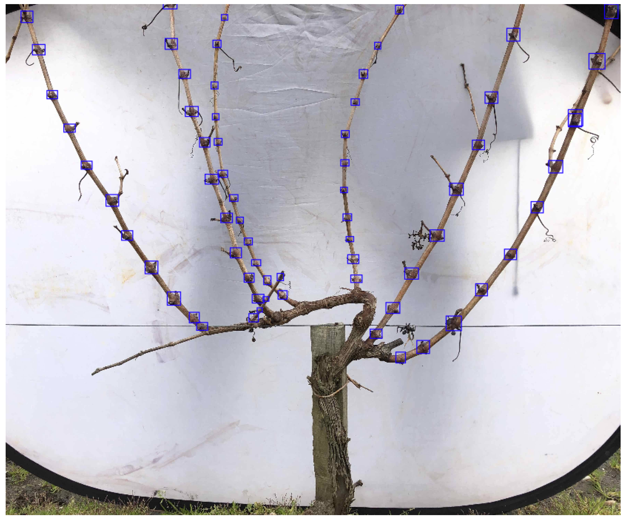
New annotations to the existing dataset have been performed to only consider the nodes on the primary canes of the grapevine in the centre of each image, which are the main detection goal, since pruning will be conducted on these primary canes considering as criteria the number of nodes present. This step was performed to guarantee it was achieved lightweight models for node detection by removing non-relevant information on the detection framework, such as nodes in areas of the grapevine not corresponding to primary canes. These annotations were performed using the Computer Vision Annotation Tool (CVAT)
1 platform, with bounding boxes surrounding the portions of the canes containing the nodes, as seen in
Figure 1.
To comprehensively assess the resilience of the deep learning models proposed in this study to varying grapevine conditions, particularly those with cluttered backgrounds, it became imperative to curate new datasets distinct from the 3D2cut Single Guyot dataset [
11], mainly containing images without artificial backgrounds. Thus, images from two distinct Portuguese viticulture regions were used to improve this evaluation. The first set of images was gathered on
Centro de Estudos Vitivinícolas do Dão -
Dão region (40°31’31.5"N 7°51’22.7"W) and the second set was obtained on
Quinta do Seixo -
Douro region (41°10’05.4"N 7°33’17.5"W). It was considered relevant to study the performance of the trained YOLO models on images from these two sites, since the grapevine configuration is different from the 3D2cut Single Guyot dataset [
11]. Also, these images were captured without using artificial backgrounds on regions with distinct background environment information due to natural light sources and landscape, which might influence on the outcome of the detection.
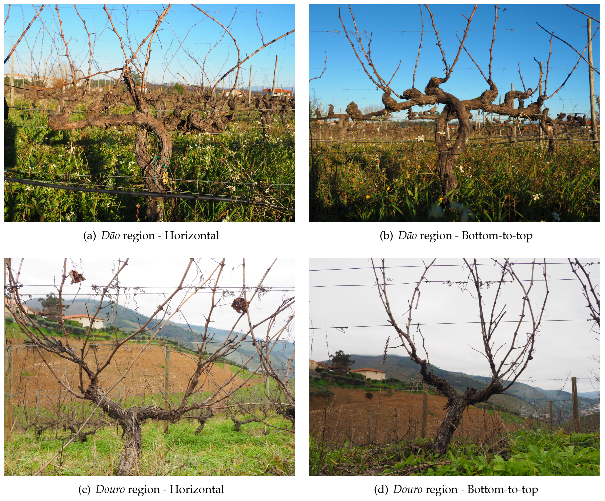
On both of these two sets of collected images, it was considered two variations on the camera’s perspective in relation to the grapevine for further performance comparison. Firstly, a horizontal perspective, which allowed the background of the image to have more objects in sight, such as adjacent vineyard lines and hills, and, afterwards, a bottom-to-top perspective with the sky being used as a more uniform background of the image, as seen in
Figure 2. The images were acquired using a digital OM System camera
2 and have a resolution of 4608×3456 pixels (px).
2.2. Deep Learning Models
YOLO deep learning models have been widely used on real-time object detection, being applied in various fields including robotics [
19]. These models are single-stage objective detection algorithms, which confer them high speed combined with precision [
20]. Due to the detection performance reported by their respective authors on the Microsoft Common Objects in Context (MS COCO) dataset [
21], the following state-of-the-art YOLO versions were selected for this work.
YOLOv7 was published in 2022 and at the time surpassed the previously developed object detectors in terms of speed and accuracy. This accuracy was improved without incrementing the inference speed, having the cost of increased training time [
22]. The authors also designed a version of this model for running in edge devices, the YOLOv7-tiny [
13], and since the goal of this work was to study detection algorithms capable of real-time inference on an autonomous robotic system, this version was chosen as one of the models for this purpose.
The YOLOv8 is one of the most recent object detection models, released in 2023. It has a backbone similar to the one used on YOLOv5 [
23] with modifications that allowed improvements on detection accuracy [
22]. Moreover, the YOLOv8 uses Distribution Focal Loss (DFL) [
24] and Complete Intersection over Union (CIoU) [
25] loss functions for the bounding-box loss which also was expected to contribute to improving the object detection performance in smaller objects [
22], being relevant for the node detection scenario due to the size of the nodes when compared to the full image of a grapevine. In order to guarantee the model used was light computing, capable of being implemented on a real-time object detection system, the model used was the YOLOv8 Small (YOLOv8s), which is the second-smallest scaled version of the model provided by Ultralytics
3. Furthermore, there have been already previous works developed on bud detection based on this version of the YOLOv8 model. Xie
et al. [
20] implemented the YOLOv8s to detect buds on tea trees, achieving a Mean Average Precision (mAP) of 88.27 % and an inference time of 37.1 ms.
In 2024, the YOLOv9 was published by the same authors of the YOLOv7. The authors designed a novel lightweight network architecture called Generalized Efficient Layer Aggregation Network (GELAN), which combined with the concept of Programmable Gradient Information (PGI), also developed by the same authors, allowed to surpass the performance of the existing object detectors. The PGI framework on the GELAN architecture helped reduce the information bottleneck during the feedforward process, which resulted in more retained complete information when compared to architectures such as PlainNet, ResNet and CSPNet [
15]. In order to compare the performance of this novel YOLO model in grapevine node detection with the previously presented ones, it was used the light computing YOLOv9 Small (YOLOv9-S).
Also in 2024, the YOLOv10 was announced with a novel approach for real-time object detection, eliminating the use of non-maximum suppression (NMS). The model is based on the YOLOv8 from Ultralytics, which the authors have chosen due to the efficient balance achieved between latency and accuracy. Despite being based on the YOLOv8, according to the authors, the YOLOv10 achieves higher average precision (AP) while requiring less parameters, fewer calculations and achieving lower latencies. The YOLOv10 was developed containing dual label assignments, which during the training phases recurs to two heads to optimize the model. However, during inference, only one head is maintained (one-to-one) to make predictions, avoiding using NMS in post-processing. Similarly to the previous ones, the model used was the small variant, the YOLOv10 Small (YOLOv10-S).
2.3. Training Configuration and Augmentations
The four distinct YOLO models presented were trained on a total of 13 539 images of grapevines, being 759 of the images from the 3D2cut Single Guyot dataset [
11] and the remaining 12 780 images resulting from augmentations of these original images.
The 3D2cut Single Guyot dataset [
11] contain varied images of grapevines with significant differences between vines not only on their main structure but also on cane orientation and size. However, this dataset is not a complete representation of possible environments and scenarios in a real-life application, lacking variations on the image capture perspective as well as external elements that might be present in the field. To address the lack of variability in this dataset, the following augmentations presented in
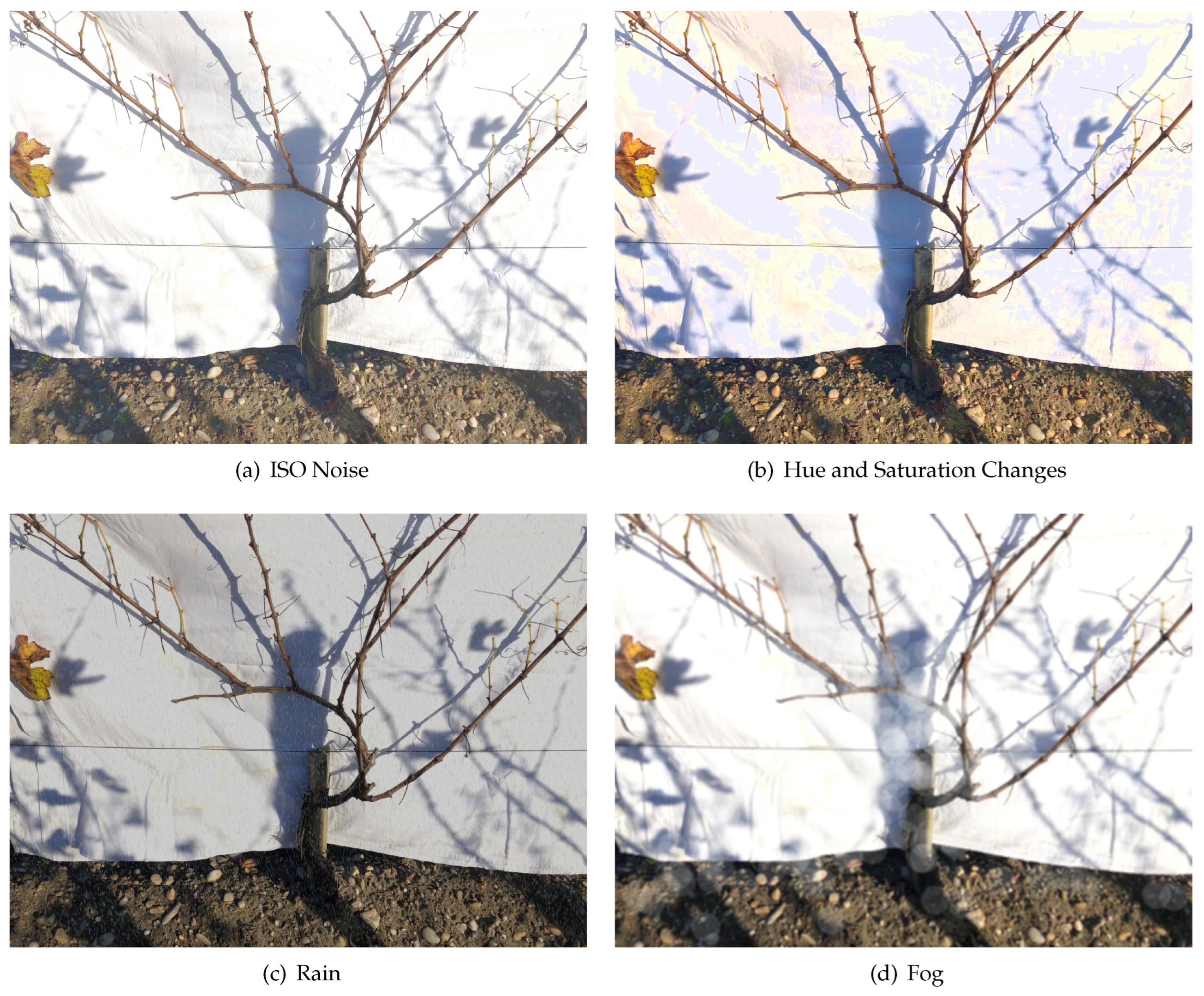
Table 1 were implemented. These augmentations used to improve the training image set presented geometric modifications to the existing dataset (image flip, scaling, and angle change), and also inserted some external elements that can be present in real-life applications on the field, such as rain, mud, fog, blur, variations in hue and saturation, ISO noise, and optical distortion, as can be seen in
Figure 3. These altered images allowed to transform the dataset to a more reliable approximation of the agricultural work environment, which is often unpredictable and subjected to harsh and variable climatic conditions [
26,
27].
The deep learning models used were initially trained with similar hyperparameters for 50 epochs. However, there was lack of convergence on the training loss for all the models. Therefore, the number of training epochs were gradually incremented to 150 for all the models to guarantee that the training loss value stabilised. Despite being used similar hyperparameters in the first conducted trainings, eventually a few suffered different tuning strategies to guarantee that the best results from each model were achieved as well as to ensure correct adaptation to the hardware used. Parameters such as input and batch sizes had to be modified on all models due to constraints on the hardware of the device used for training (NVIDIA GeForce RTX 3090
4). However, YOLOv8s, YOLOv9-S and YOLOv10-S presented more difficulties to reach convergence during training. For this purpose, Cosine learning Rate Scheduler Function [
28] was activated during training, as well as mosaic data augmentation was deactivated on the last 50 epochs to improve loss stabilization on the last training stages. Furthermore, different optimisers were tested on different trainings, and it was discovered that on all the models tested the AdamW contributed to better convergence. The basic configurations of the models, as well as the hyperparameters that suffered further modifications in each deep learning model used, resulting in the most favourable results, can be seen in
Table 2.
3. Results
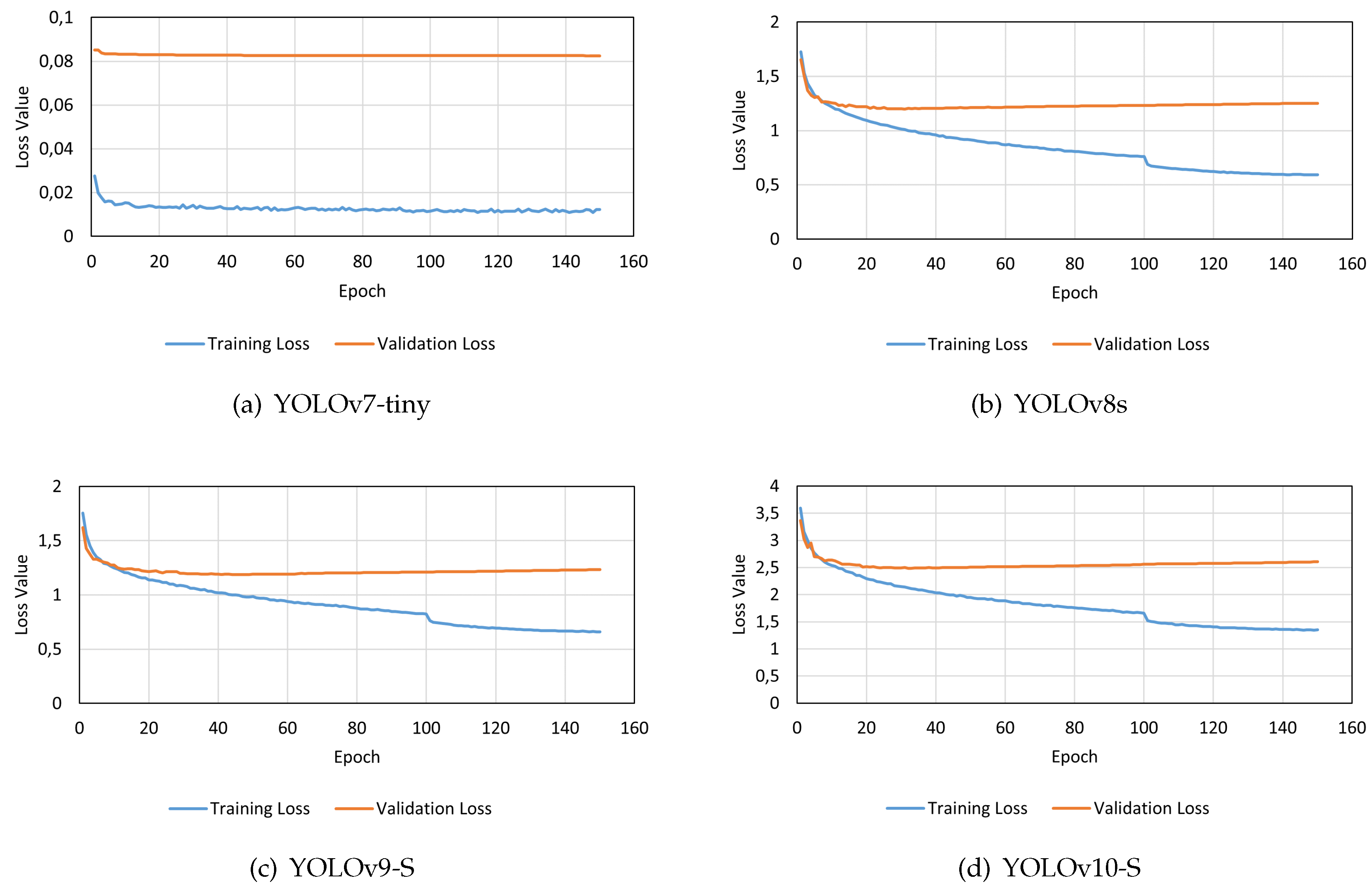
The trained YOLO models demonstrated convergence within the 150 epochs of training. However, the YOLOv7-tiny resulted in smaller box-loss values for both training and validation, as well as those values were more stable at the end of the training when compared to the other models. The other models started to present a slight increase in the validation loss, which can be an indicator the model is starting to overfit [
29]. In contrast, YOLOv10-S exhibited higher loss values during training compared to the other models. The box loss values of the models trained are presented in
Figure 4.
3.1. Validation and Field Trials
Three different sets of images were selected to evaluate the performance of the models in detecting the nodes on grapevines. The first set was composed of images from the 3D2cut Single Guyot dataset [
11], containing an artificial background behind the captured grapevines. The remaining two sets consisted of images selected from the datasets gathered on the Portuguese
Dão and
Douro regions, containing 30 original images and 150 augmented images, which added geometric modifications to the original images in order to increase the variability of the dataset by containing grapevines captured in different layouts.
The images from the 3D2cut Single Guyot dataset [
11] were used as a benchmark to compare the robustness of the YOLO models trained. Since these images were similar to the ones used for training, it was expected that the models would achieve the best results on them.
Dão and
Douro datasets were constituted of images taken in open fields without covering the objects behind the grapevines. This feature allowed these datasets to be used as indicators to evaluate the robustness of the models developed in detecting nodes on images with natural backgrounds (cluttered).
Furthermore, despite the models have been trained with an input size of 640×640 px, it was also conducted tests with changes in the input parameter to consider a size of 1280×1280 px. Since nodes on grapevines are relatively small objects on the overall size of the image, this test was crucial to reduce the loss of information on the images used. However, it was expected that this increase in the input size would result in delays in the inference times of the models [
30].
The results obtained on the validation phase of the detection models trained on the four different datasets can be seen in
Table 3. The metrics obtained were analysed at confidence levels of at least 10 % and at the best F1-Score obtained in each model. Values of confidence lower than 10 % were not considered in the results, since these low values would not be appropriate to consider for a real case implementation of a perception module for a pruning robot. Furthermore,
Table 4 displays the average inference time per image on each of the models with different input sizes.
4. Discussion
Overall, YOLOv7-tiny achieved higher F1-Score values than the other models. The more recent models tested, despite typically presenting slightly higher Precision values, resulted in lower Recall values. Moreover, the mAP obtained by the novel YOLOv10-S was usually significantly lower than the other models benchmarked for scenarios significantly different from the training environment.
Observing the results previously presented in
Table 3, there was a tendency for the models to perform better with an input size of 1280×1280 px when compared to the standard input size of 640×640 px, which supports the possibility of information being lost in smaller images due to the reduced size of the nodes. Due to this characteristic, it was considered advantageous to use this larger input size on the developed models, which demonstrated performance improvements.
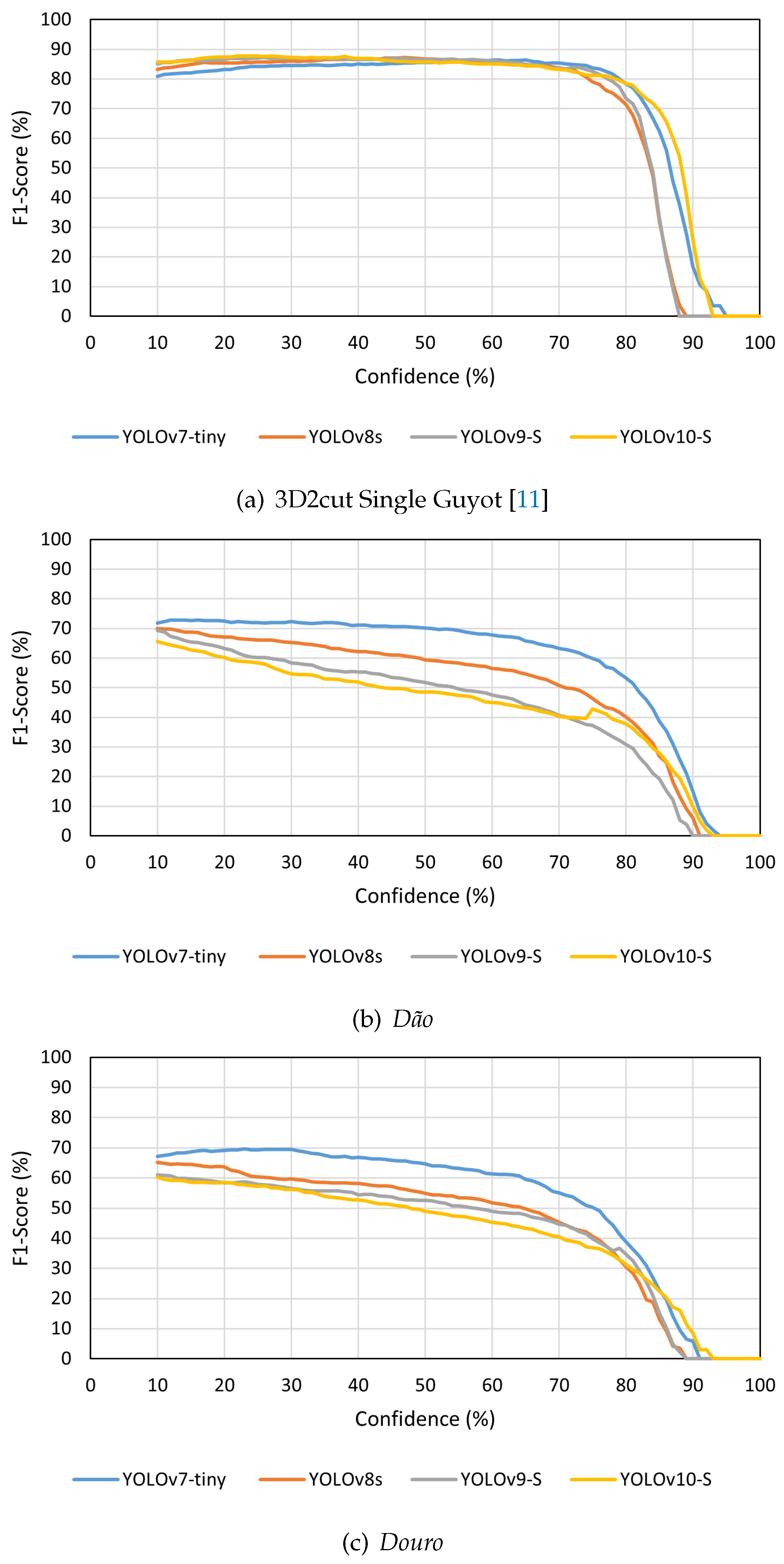
Figure 5 shows a comparison of the F1-Score values from the four YOLO models analysed on the different datasets used, considering an input size of 1280×1280 px.
Despite these performance differences between the used versions, all the models were capable of detecting grapevine’s nodes successfully. Furthermore, it was possible to observe that on the 3D2cut Single Guyot dataset [
11], the four models achieved F1-Score values of above 80 %, despite the input size used. Meanwhile, on both
Dão and
Douro datasets, the highest F1-Score values were around 70 %. However, since the objective of this study is to further implement a perception algorithm on a robotic system capable of performing pruning tasks autonomously, not only is crucial to analyse the models’ accuracy and their adaptability to different real case scenarios, but also how much time they take to complete the inference.
4.1. Adaptability to Different Grapevine’s Configurations And Environments
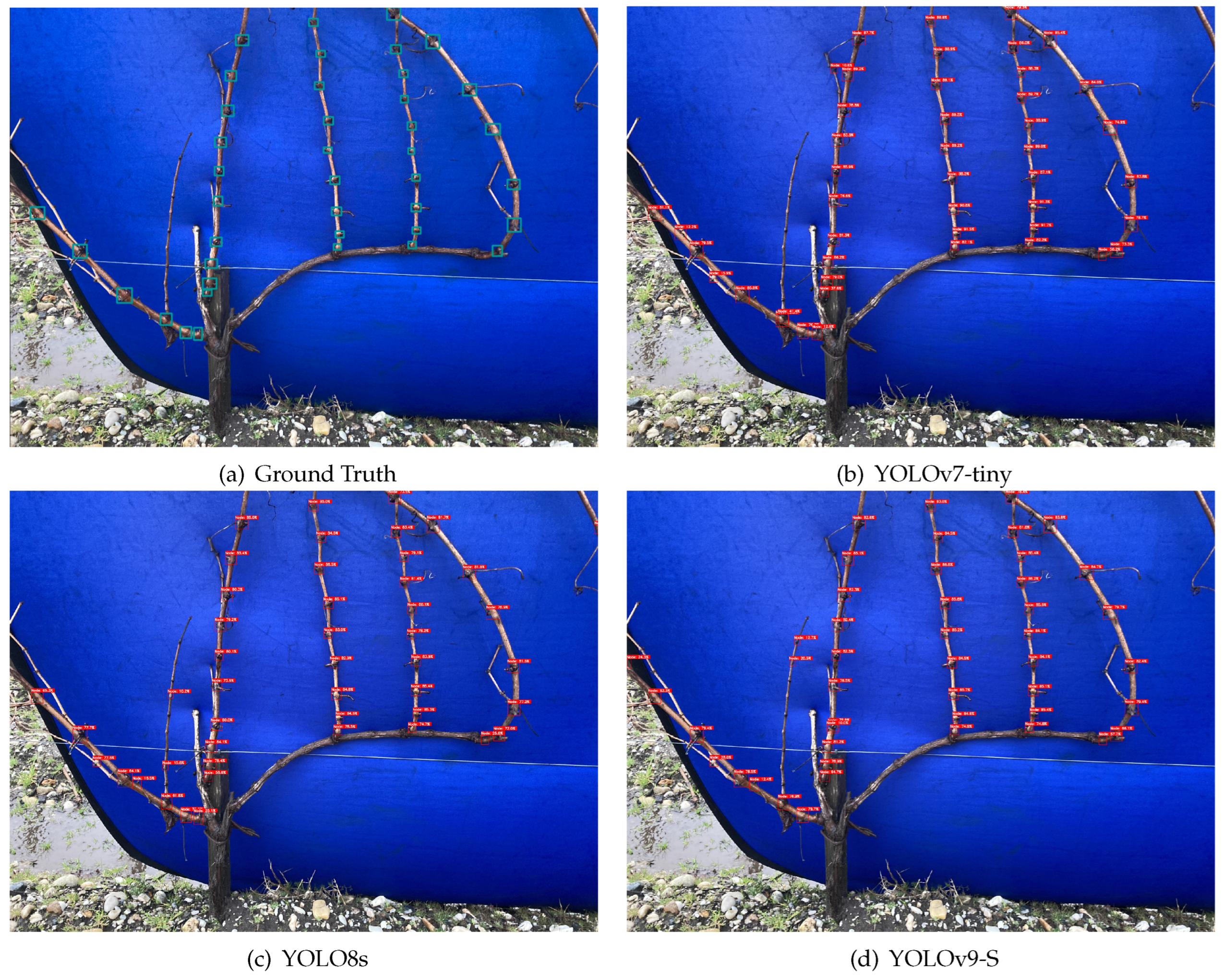
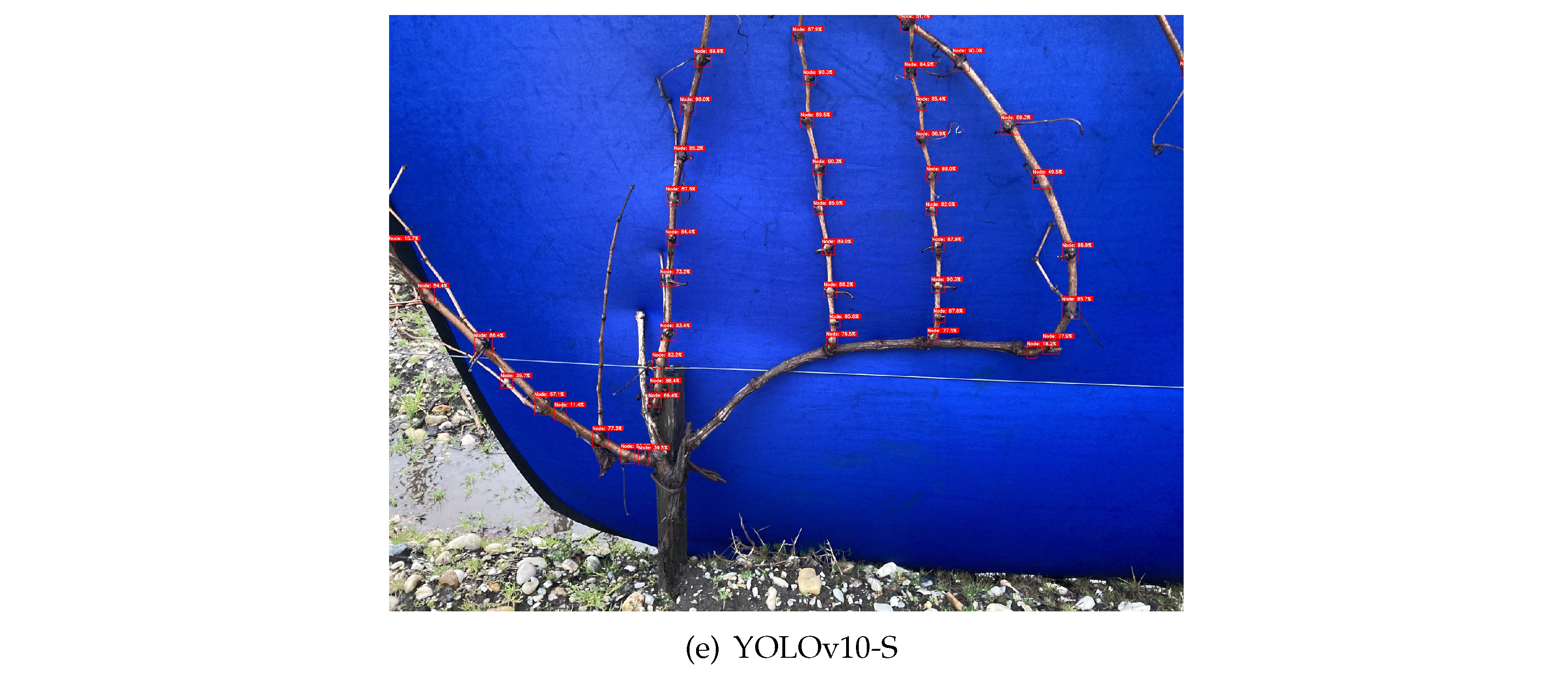
As expected, the models’ inference performance was considerably higher on the 3D2cut Single Guyot dataset [
11], where all the models presented a similar detection capability, as seen in
Figure 6. This behaviour occurs not only because this set was constituted of images similar to the ones used for training, but also due to the amount of additional information on the background of the
Dão and
Douro datasets, which induced the occurrence of some false positive detections on the background of the images.
In both of these other two datasets (
Dão and
Douro) was possible to notice that the YOLOv7-tiny achieved higher F1-Score values than the other three models, being this difference more noticeable on these datasets in comparison to the results obtained on the 3D2cut Single Guyot dataset [
11]. Furthermore, despite YOLOv8s being the second best performing model on
Dão dataset, the performance changes significantly on
Douro dataset, in which this model presents varying results according to the input size used, resulting in lower F1-Score values for input size of 640×640 px. Despite the Precision of YOLOv10-S being usually higher than the other models on the Portuguese datasets, the Recall was lower, specially when considering an input size of 640×640 px. This allowed to notice that when using the YOLOv10-S, despite not occurring many false positives, the model presents more difficulties in detecting small objects on each frame, ignoring a few nodes in the image. This behaviour makes it less valuable for the intended task than the other models analysed, since this behaviour results in a considerable amount of nodes not being considered as such.
Furthermore, when comparing the results obtained between the two datasets without artificial background, the
Douro dataset resulted in less accurate detections by the models than the
Dão dataset. Analysing the images present in each one, it is possible to observe what features might be causing this discrepancy. The grapevines on
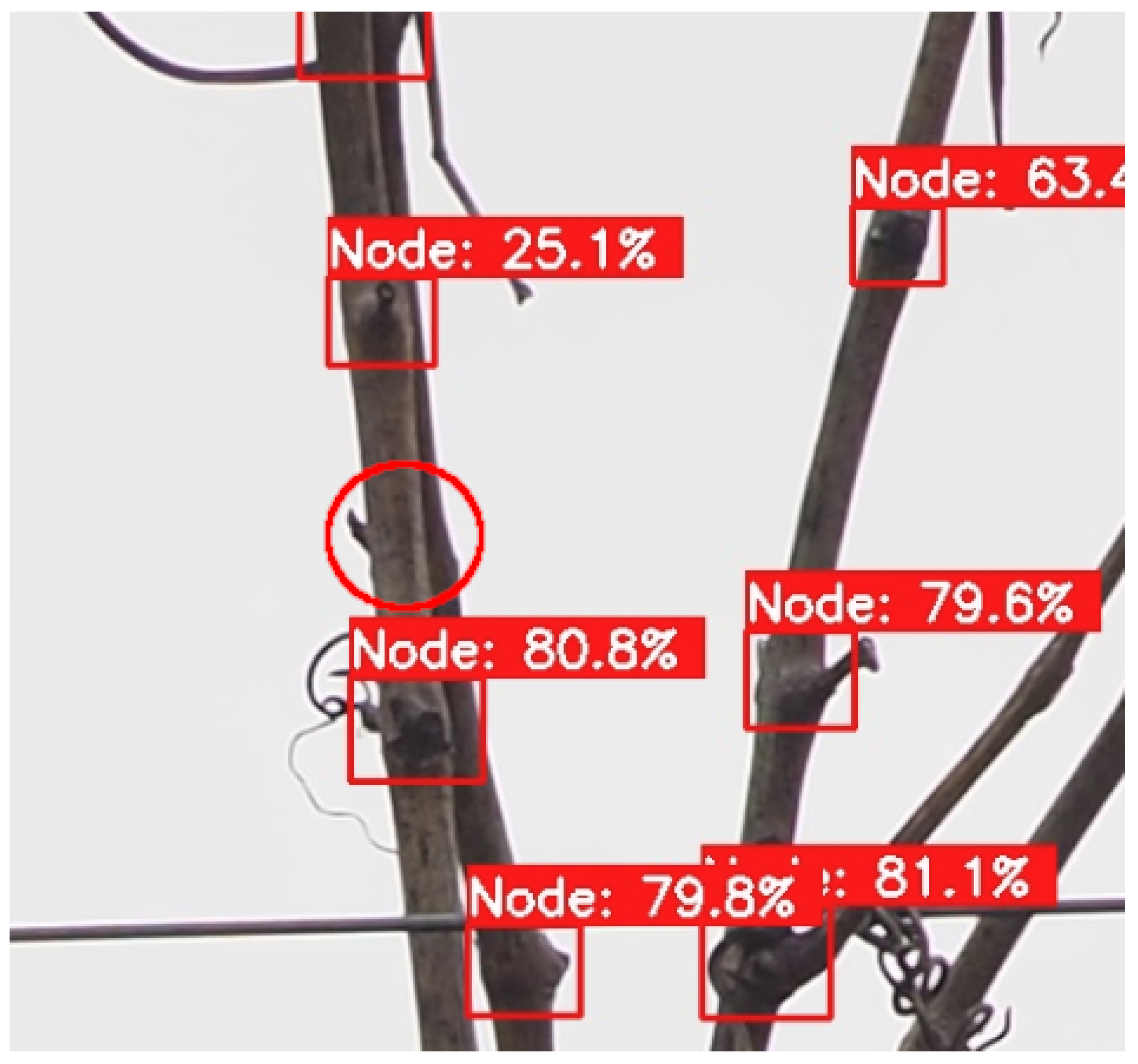
Dão dataset, despite having a structure different from the grapevines on the images of the training dataset, distinguishing each cane on the plant is still easily feasible. Meanwhile, on
Douro dataset, the grapevines have more canes overlapped, being sometimes more difficult to distinguish the primary canes and also resulting in nodes to be occluded by nearby branches, as can be observed in
Figure 7.
Regarding the annotations performed on the 3D2cut Single Guyot dataset [
11], only the nodes on the primary canes of the centred grapevine on the image were selected. The same logic was implemented on the construction of the ground truth for the
Dão and
Douro image sets. However, the models also detected a few nodes on canes in adjacent grapevines that slightly appeared on the images captured. This consequently resulted in these detections being considered as false positives, which is not entirely wrong since the nodes do not belong to the focused grapevine, but they are correctly assumed as being nodes. Although these situations slightly affect some of the images, they were not considered relevant for the overall performance of the models in detecting nodes on these datasets, since only happened on a few cases. Furthermore, on these sets of images taken in open field, the pictures captured on a bottom-to-top perspective are preferable to achieve better results. This approach helped reduce the background information, resulting in less false positives detected.
Regardless of the performance differences between datasets and between images containing or not artificial background, grapevine node detection recurring to YOLO detection models presents an efficient and more versatile approach when compared to the previously implemented methods. The previously published work by Gentilhomme
et al. [
11] considered that algorithms proposed for pruning assistance would be severely impacted in work conditions without uniform backgrounds. However, this work assures that grapevine node detection is feasible in heterogeneous environments recurring to state-of-the-art YOLO detection models, despite occurring a slight performance decrease.
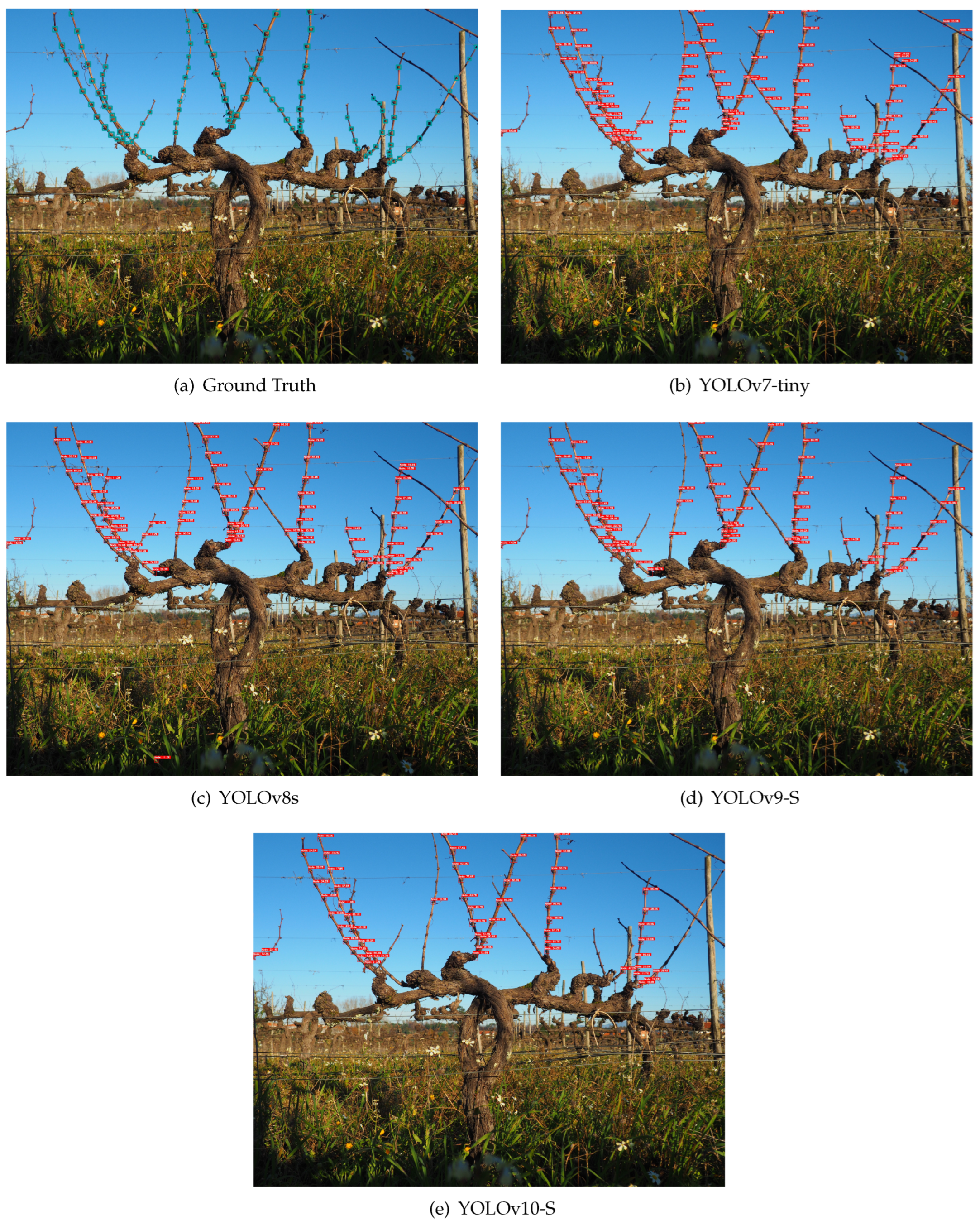
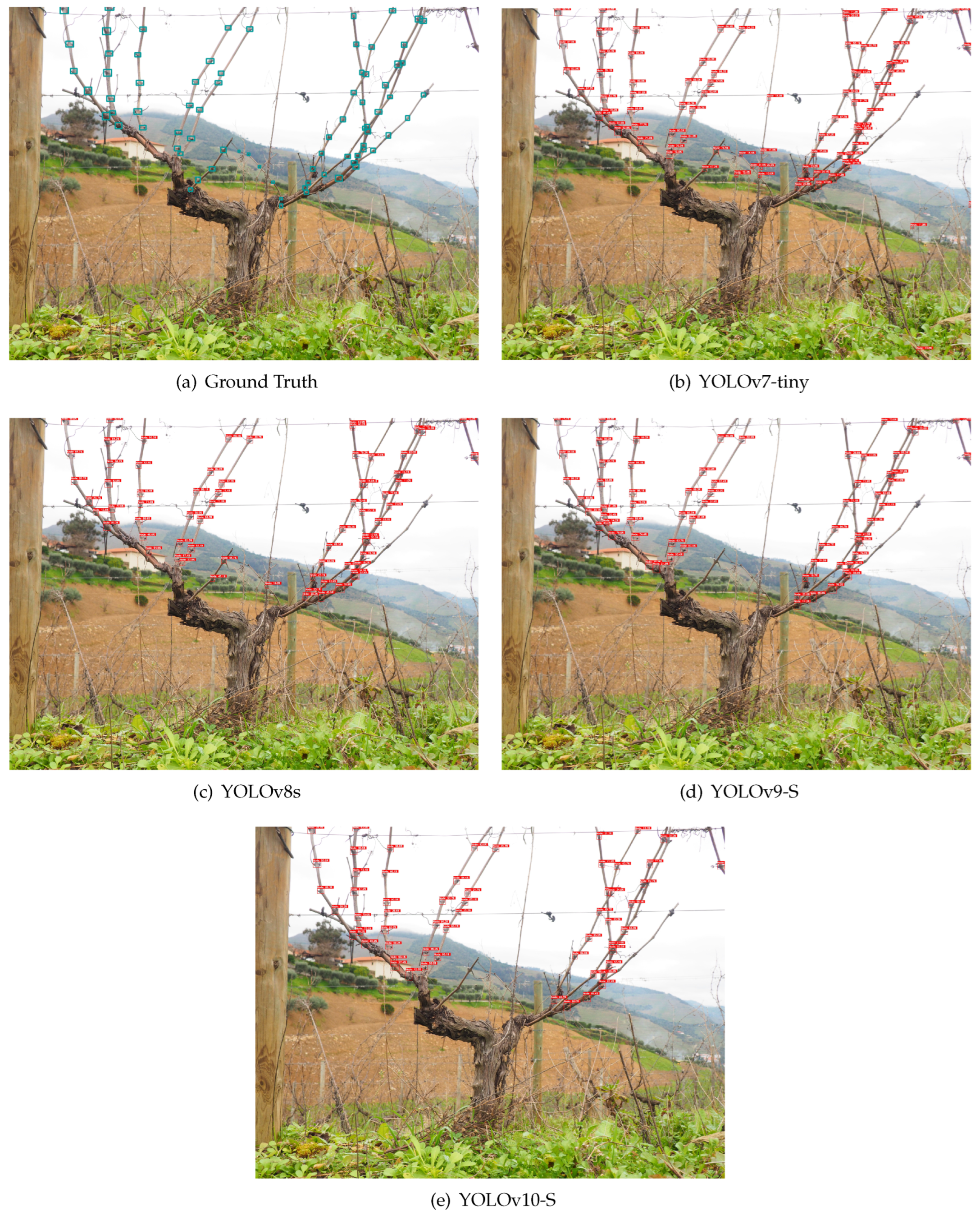
Furthermore, it was possible to assess the capability of performing node detection on the entirety of the grapevines even when configurations different from those used in training are provided to the models. In
Figure 8 and
Figure 9 is possible to analyse the inference behaviour of the models used on each of the datasets acquired in Portugal,
Dão and Douro, respectively, considering an input size of 1280×1280 px.
4.2. Capability of Implementation in a Real-Time System
According to the work by Botterill
et al. [
1], a human takes approximately 2 minutes to prune a grapevine. In a robotic system, there might be necessary several additional steps from the detection of the cutting location until the cut is completed. These steps are mainly related to navigation towards the cutting location and actuation of the cutting tool [
7,
31]. Considering this, minimizing the inference time of the detection algorithm is crucial to ensure the maximum efficiency of the system by reducing the necessary time to execute the pruning task on each vine.
The average inference time of the analysed YOLO models varied significantly. These inference time differences were not only between the distinct versions of the models, but also between different input sizes. YOLOv7-tiny was the fastest model at grapevine node detection, presenting inference times below 100 ms. YOLOv8s, YOLOv9-S and YOLOv10-S presented significantly larger times, with YOLOv8s reaching an average of around 502.5 ms when detecting nodes with a 1280×1280 px input size.
Despite the most recent models (YOLOv9-S and YOLOv10-S) being faster than the 502 ms of YOLOv8s, their inference times on 1280×1280 px sized images is still near 300 ms, which is significantly higher than the inference time obtained using the YOLOv7-tiny. Considering this, in matter of capability of implementation in a real-time system, the YOLOv7-tiny would be the preferable model of the four in order to ensure the system’s efficiency.
5. Conclusions
This work allowed to compare side-by-side four distinct YOLO models on the capability of successfully performing the task of node detection in grapevine’s canes. The models were trained on the publicly available 3D2cut Single Guyot dataset, which contained an artificial background on the captured images. Furthermore, the models were tested on two different Portuguese grapevine datasets without artificial backgrounds, which allowed to evaluate the robustness of the models on two distinct cultivars with different surrounding environments.
Considering this approach, it was possible to notice that YOLOv7-tiny achieved the best detection performance compared to the other used models. Furthermore, YOLOv7-tiny was the best model considering the trade-off between accuracy and inference speed. This detection model not only achieved overall better metrics compared to the state-of-the-art detection models, but also presented the fastest inference speed for both tested input sizes (640×640 px and 1280×1280 px).
Despite the significant performance variation between solutions, all the state-of-the-art YOLO models used are capable of detecting the nodes on grapevines even when additional environment information is present on the background of the frames behind the vines, being an improvement to previously developed algorithms that lacked robustness to actuate in heterogeneous environments. This approach of node detection recurring to YOLO detection models fulfilled the objectives of presenting efficient and light computing deep learning models for node detection on 2D images of grapevines. These models are capable of detecting nodes in cluttered environments when visualising the entire grapevine, as well as confer inference times compatible with a real-time system implementation.
However, despite being proven the feasibility of implementing YOLO detecting models on these type of environments, as future work, it would be interesting to perform the detections by firstly filtering the background of the images using data from a depth camera to remove unwanted information, which is expected to also improve inference times since the information available for inference will be reduced.
Author Contributions
Conceptualisation, F.O., D.Q.S. and V.F.; Data curation, F.O. and D.Q.S.; Funding acquisition, F.N.S.; Investigation, F.O. and D.Q.S.; Methodology, F.O. and D.Q.S.; Project administration, F.N.S.; Software, F.O. and D.Q.S.; Supervision, T.M.P., J.B.C. and F.N.S.; Validation, V.F., T.M.P., M.C., J.B.C. and F.N.S.; Visualisation, F.O.; Writing - original draft, F.O.; writing - review and editing, D.Q.S., V.F., T.M.P., M.C., J.B.C. and F.N.S. All authors read and agreed to the published version of the manuscript.
Funding
This research received no external funding.
Institutional Review Board Statement
Not applicable.
Informed Consent Statement
Not applicable.
Data Availability Statement
Acknowledgments
The authors would like to acknowledge this work is co-financed by Component 5 - Capitalization and Business Innovation, integrated in the Resilience Dimension of the Recovery and Resilience Plan within the scope of the Recovery and Resilience Mechanism (MRR) of the European Union (EU), framed in the Next Generation EU, for the period 2021 - 2026, within project Vine&Wine_PT, with reference 67. The authors would like to thank Centro de Estudos Vitivinícolas do Dão and Sogrape for making their vineyards available for data acquisition.
Conflicts of Interest
The authors declare no conflicts of interest. The funders had no role in the design of the study; in the collection, analyses, or interpretation of data; in the writing of the manuscript; or in the decision to publish the results.
Abbreviations
The following abbreviations are used in this manuscript:
| 2D |
Two-dimensional |
| AP |
Average Precision |
| CIoU |
Complete Intersection over Union |
| CNN |
Convolutional Neural Network |
| CVAT |
Computer Vision Annotation Tool |
| DFL |
Distribution Focal Loss |
| FCN |
Fully Convolutional Network |
| GELAN |
Generalized Efficient Layer Aggregation Network |
| mAP |
Mean Average Precision |
| MS COCO |
Microsoft Common Objects in Context |
| NMS |
Non-Maximum Suppression |
| PGI |
Programmable Gradient Information |
| SHG |
Stacked Hourglass Network |
| YOLO |
You Only Look Once |
References
- Botterill, T.; Paulin, S.; Green, R.D.; Williams, S.; Lin, J.; Saxton, V.; Mills, S.; Chen, X.; Corbett-Davies, S. A Robot System for Pruning Grape Vines. Journal of Field Robotics 2017, 34. [Google Scholar] [CrossRef]
- Poni, S.; Sabbatini, P.; Palliotti, A. Facing Spring Frost Damage in Grapevine: Recent Developments and the Role of Delayed Winter Pruning – A Review. American Journal of Enology and Viticulture 2022, 73, 211–226. [Google Scholar] [CrossRef]
- Reich, L. The Pruning Book; Taunton Press, 2010.
- Silwal, A.; Yandun, F.; Nellithimaru, A.; Bates, T.; Kantor, G. Bumblebee: A Path Towards Fully Autonomous Robotic Vine Pruning, 2021, [arXiv:cs.RO/2112.00291].
- Williams, H.; Smith, D.; Shahabi, J.; Gee, T.; Nejati, M.; McGuinness, B.; Black, K.; Tobias, J.; Jangali, R.; Lim, H.; Duke, M.; Bachelor, O.; McCulloch, J.; Green, R.; O’Connor, M.; Gounder, S.; Ndaka, A.; Burch, K.; Fourie, J.; Hsiao, J.; Werner, A.; Agnew, R.; Oliver, R.; MacDonald, B.A. Modelling wine grapevines for autonomous robotic cane pruning. Biosystems Engineering 2023, 235, 31–49. [Google Scholar] [CrossRef]
- Oliveira, F.; Tinoco, V.; Magalhães, S.; Santos, F.N.; Silva, M.F. End-Effectors for Harvesting Manipulators - State Of The Art Review. 2022 IEEE International Conference on Autonomous Robot Systems and Competitions (ICARSC), 2022, pp. 98–103. [CrossRef]
- He, L.; Schupp, J. Sensing and Automation in Pruning of Apple Trees: A Review. Agronomy 2018, 8. [Google Scholar] [CrossRef]
- Collins, C.; Wang, X.; Lesefko, S.; De Bei, R.; Fuentes, S. Effects of canopy management practices on grapevine bud fruitfulness. OENO One 2020, 54, 313–325. [Google Scholar] [CrossRef]
- Cuevas-Velasquez, H.; Gallego, A.J.; Tylecek, R.; Hemming, J.; Van Tuijl, B.; Mencarelli, A.; Fisher, R.B. Real-time Stereo Visual Servoing for Rose Pruning with Robotic Arm. 2020, p. 7050 – 7056. [CrossRef]
- Villegas Marset, W.; Pérez, D.S.; Díaz, C.A.; Bromberg, F. Towards practical 2D grapevine bud detection with fully convolutional networks. Computers and Electronics in Agriculture 2021, 182, 105947. [Google Scholar] [CrossRef]
- Gentilhomme, T.; Villamizar, M.; Corre, J.; Odobez, J.M. Towards smart pruning: ViNet, a deep-learning approach for grapevine structure estimation. Computers and Electronics in Agriculture 2023, 207, 107736. [Google Scholar] [CrossRef]
- Redmon, J.; Divvala, S.; Girshick, R.; Farhadi, A. You Only Look Once: Unified, Real-Time Object Detection. 2016 IEEE Conference on Computer Vision and Pattern Recognition (CVPR), 2016, pp. 779–788. [CrossRef]
- Wang, C.; Bochkovskiy, A.; Liao, H. YOLOv7: Trainable Bag-of-Freebies Sets New State-of-the-Art for Real-Time Object Detectors. 2023 IEEE/CVF Conference on Computer Vision and Pattern Recognition (CVPR); IEEE Computer Society: Los Alamitos, CA, USA, 2023; pp. 7464–7475. [Google Scholar] [CrossRef]
- Jocher, G.; Chaurasia, A.; Qiu, J. Ultralytics YOLOv8 2023.
- Wang, C.Y.; Liao, H.Y.M. YOLOv9: Learning What You Want to Learn Using Programmable Gradient Information 2024.
- Wang, A.; Chen, H.; Liu, L.; Chen, K.; Lin, Z.; Han, J.; Ding, G. YOLOv10: Real-Time End-to-End Object Detection, 2024, [arXiv:cs.CV/2405.14458].
- Lavrador da Silva, A..; João Fernão-Pires, M..; Bianchi-de-Aguiar, F.. Portuguese vines and wines: heritage, quality symbol, tourism asset. Ciência Téc. Vitiv. 2018, 33, 31–46. [CrossRef]
- Oliveira, F.A.; Silva, D.Q. Douro & Dão Grapevines Dataset for Node Detection, 2024. [CrossRef]
- Casas, G.G.; Ismail, Z.H.; Limeira, M.M.C.; da Silva, A.A.L.; Leite, H.G. Automatic Detection and Counting of Stacked Eucalypt Timber Using the YOLOv8 Model. Forests 2023, 14. [Google Scholar] [CrossRef]
- Xie, S.; Sun, H. Tea-YOLOv8s: A Tea Bud Detection Model Based on Deep Learning and Computer Vision. Sensors 2023, 23. [Google Scholar] [CrossRef] [PubMed]
- Lin, T.Y.; Maire, M.; Belongie, S.; Bourdev, L.; Girshick, R.; Hays, J.; Perona, P.; Ramanan, D.; Zitnick, C.L.; Dollár, P. Microsoft COCO: Common Objects in Context, 2015, [arXiv:cs.CV/1405.0312].
- Terven, J.; Córdova-Esparza, D.M.; Romero-González, J.A. A Comprehensive Review of YOLO Architectures in Computer Vision: From YOLOv1 to YOLOv8 and YOLO-NAS. Machine Learning and Knowledge Extraction 2023, 5, 1680–1716. [Google Scholar] [CrossRef]
- Jocher, G. YOLOv5 by Ultralytics 2020. [CrossRef]
- Li, X.; Wang, W.; Wu, L.; Chen, S.; Hu, X.; Li, J.; Tang, J.; Yang, J. Generalized focal loss: learning qualified and distributed bounding boxes for dense object detection. Proceedings of the 34th International Conference on Neural Information Processing Systems; Curran Associates Inc.: Red Hook, NY, USA, 2020; NIPS’20. [Google Scholar]
- Zheng, Z.; Wang, P.; Liu, W.; Li, J.; Ye, R.; Ren, D. Distance-IoU Loss: Faster and Better Learning for Bounding Box Regression. Proceedings of the AAAI Conference on Artificial Intelligence 2020, 34, 12993–13000. [Google Scholar] [CrossRef]
- Vougioukas, S.G. Agricultural Robotics. Annual Review of Control, Robotics, and Autonomous Systems 2019, 2, 365–392. [Google Scholar] [CrossRef]
- Bechar, A.; Vigneault, C. Agricultural robots for field operations: Concepts and components. Biosystems Engineering 2016, 149, 94–111. [Google Scholar] [CrossRef]
- Hsueh, B.Y.; Li, W.; Wu, I.C. Stochastic Gradient Descent With Hyperbolic-Tangent Decay on Classification. 2019 IEEE Winter Conference on Applications of Computer Vision (WACV), 2019, pp. 435–442. [CrossRef]
- Prechelt, L., Early Stopping - But When? In Neural Networks: Tricks of the Trade; Orr, G.B.; Müller, K.R., Eds.; Springer Berlin Heidelberg: Berlin, Heidelberg, 1998; pp. 55–69. [CrossRef]
- Butko, N.J.; Movellan, J.R. Optimal scanning for faster object detection. 2009 IEEE Conference on Computer Vision and Pattern Recognition, 2009, pp. 2751–2758. [CrossRef]
- Zahid, A.; Mahmud, M.S.; He, L.; Heinemann, P.; Choi, D.; Schupp, J. Technological advancements towards developing a robotic pruner for apple trees: A review. Computers and Electronics in Agriculture 2021, 189, 106383. [Google Scholar] [CrossRef]
|
Disclaimer/Publisher’s Note: The statements, opinions and data contained in all publications are solely those of the individual author(s) and contributor(s) and not of MDPI and/or the editor(s). MDPI and/or the editor(s) disclaim responsibility for any injury to people or property resulting from any ideas, methods, instructions or products referred to in the content. |
© 2024 by the authors. Licensee MDPI, Basel, Switzerland. This article is an open access article distributed under the terms and conditions of the Creative Commons Attribution (CC BY) license (https://creativecommons.org/licenses/by/4.0/).
