The Application of Deep Learning to Accurately Identify the Dimensions of Spinal Canal and Intervertebral Foramen as Evaluated by the IoU Index

Artificial intelligence has garnered significant attention in recent years as a rapidly advancing field of computer technology. With the continual advancement of computer hardware, deep learning has made breakthrough developments within the realm of artificial intelligence. Over the past few years, applying deep learning architecture in medicine and Industrial anomaly inspection has significantly contributed to solving numerous challenges related to efficiency and accuracy. Despite excellent results in radiological, pathological, endoscopic, ultrasonic, and biochemical examinations, this paper utilizes deep learning combined with image processing to identify spinal canal and vertebral foramen dimensions. In existing research, technologies such as corrosion and expansion in magnetic resonance image (MRI) processing have also strengthening the accuracy of results. Indicators such as area and Intersection over Union (IoU)are also provided for assessment. Among them, the mean average precision (mAP), for identifying intervertebral foramen (IVF) and intervertebral disc (IVD) through YOLOv4 is 95.6%. Resnet50 mixing U-Net was employed to identify the spinal canal and intervertebral foramen and achieved IoU scores of 79.11% and 80.89%.

Keywords:

Subject:

Computer Science and Mathematics - Artificial Intelligence and Machine Learning

1. Introduction

The lumbar spine is a complex anatomical structure composed of bony vertebrae, intervertebral joints, ligamentum flavum, and intervertebral discs. These elements work in concert with the paraspinal muscles to maintain the overall stability of the human body, facilitating both static posture and dynamic trunk movements. The lumbar spinal canal and intervertebral foramina provide critical protection for the dura mater and nerve roots, which are essential for motor functions of the lower limbs as well as the regulation of urinary and fecal excretion [1]. Degenerative lumbar spine disease (DLSD) is a major health problem worldwide, considered a leading cause of disability, and an issue worthy of discussion, with an estimated 266 million individuals affected globally each year [2]. DLSD includes a spectrum of conditions, such as intervertebral disc herniation, spondylolisthesis, spinal stenosis, and intervertebral foraminal stenosis. These conditions lead to lumbar instability and nerve root compression. This can clinically present as low back pain, neurogenic claudication, radiculopathy, or, in severe cases, cauda equina syndrome. [3]. To accurately diagnose DLSD, clinicians typically rely on various imaging modalities, including X-rays, Magnetic Resonance Imaging (MRI), and computed tomography (CT). The choice of imaging technique is guided by the patient’s specific symptoms, clinical signs, and neurological examination findings. Among these modalities, MRI is particularly valuable due to its high sensitivity in detecting abnormalities in lumbar soft tissues, intervertebral foramina, the ligamentum flavum, discs, and cerebrospinal fluid [4]. MRI enables the precise identification of lumbar spine lesions, allowing for prompt and appropriate intervention. However, despite the diagnostic power of MRI, interpretation can be subject to human error and variability.

Over the past twenty years, Artificial Intelligence (AI) advancements have dramatically transformed medical practice, addressing limitations in disease diagnosis, precision medicine, medical imaging, error reduction, and healthcare cost efficiency [5,6,7]. AI technologies and intense learning algorithms have shown promise in enhancing the accuracy and consistency of diagnoses, especially in complex cases involving multiple potential pain generators such as low back pain and sciatica. The development and application of AI in analyzing spinal imaging studies, including MRI, represent a growing area of interest, offering potential improvements in diagnostic precision and patient outcomes [8,9,10,11]. The spinal canal and intervertebral foraminal stenosis are key anatomical factors that contribute to the pathophysiology of low back pain and sciatica. Recognizing the importance of accurately diagnosing these conditions, we have developed an AI-driven deep learning (DL) architecture specifically designed to evaluate and analyze cross-sectional images of the spinal canal and intervertebral foramina in the lumbar spine. This model aims to enhance the diagnostic process by reducing human bias and increasing the accuracy of detecting clinically significant stenosis, thereby improving overall patient care.

2. Methods and Materials

2.1. Methods

This section describes the methods employed in our research, emphasizing the effective utilization of convolutional neural networks (CNNs), a critical subset of artificial neural networks (ANNs) [12]. ANN is the fundamental element in neural networks. Specifically, we focus on the comprehensive evaluation of distinguished CNN architectures: Visual Geometry Group (VGG),ResNet, and U-Net. To actualize our research methods, we embark on an explication of the rudimentary workings of ANNs. We start with a detailed comprehensive of the VGG and ResNet [13] and U-net models, examining three distinct attributes and their notable contributions to deep learning.

2.1.1. ResNet

Over the last few years, the sphere of deep learning (DL) has made major progress, such as medical image recognition and reinforcement learning. Amongst the miscellaneous neural network architectures that have been extended, ResNet [13] has garnered a considerable level of attention due to top-notch performance and accuracy. This revision investigates the selection of ResNet for identifying canal and foraminal stenosis, highlighting its architectural strengths and particular applications in this context. ResNet function in identifying canal and foramen l stenosis area is pivotal due to its potential to vanquish ordinary DL challenges, similar to gradient issue information will be missed. These complexes improve the network’s capability to achieve deep feature extraction and accuracy, which is crucial for accurately predicting and identifying canal and foramen l stenosis. Let

x

denote the input,

y

the output,

F (x, \{w_{i}\})

represents the residual mapping that needs to be learned. The function of a residual block in ResNet can be conveyed mathematically as

y = F (x, \{w_{i}\}) + x

(1)

2.1.2. VGG

It is a typical model of deep Convolutional Neural Network (CNN) design with a multitude of layers, and the acronym VGG [14] means Visual Geometry Group. The main contribution of this article is through the consecutive stacking of small convolutional filters (3x3), the CNN model can reach a deeper layer and acquire better accuracy and faster speed. Although this concept is simple, it is very important. At that time, there were still many questions and research on how to set the filter parameters. For example, AlexNet [15] used a considerable size (11x11), and GoogLeNet [16] also used different filter sizes. A prominent design theory of VGG is to fulfill high-accuracy performance through shallow and deep convolutional neural networks. Why does VGG [14] use 3x3 Convolutional? Because this is the smallest size that can contain surrounding information. It is believed that the substitution of a larger convolutional with a more minor convolutional can improve the receptive field (it can also be said to increase the amount of information). In addition, using smaller convolutional can improve Non-Linearity while reducing parameters in contrast with large convolutional.

2.1.3. U-Net

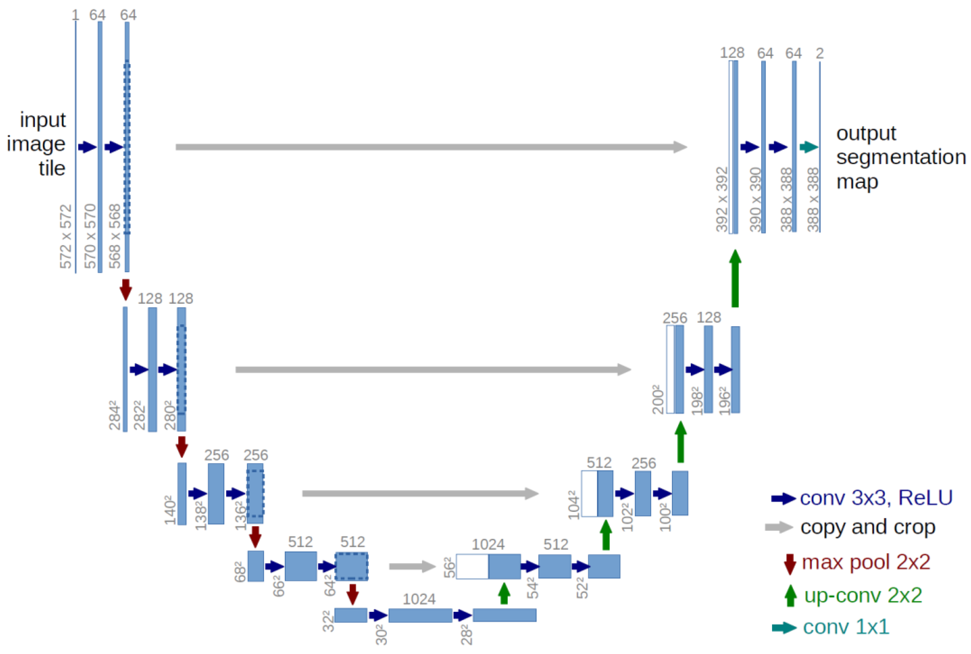
U-Net is a highly effective model for medical image segmentation tasks, such as separating cancerous tumors and segmenting biological cell nuclei. As illustrated in Figure 1, the U-Net architecture is symmetrical and U-shaped [17]. The model is mainly composed of a sequence of convolutional layers. The left segment, which forms the left side of the 'U,' functions as the Encoder, while the right segment, representing the right side of the 'U,' acts as the decoder. A critical distinction between U-Net and a typical autoencoder [18] lies in the presence of skip connections in U-Net, which connect corresponding layers in the encoder and decoder.

The U-Net architecture closely resembles an autoencoder [18], with the critical difference being that U-Net's input is an image, and its output is the segmented version of that image. Typically, the input and output images are of the same size. Figure 2 illustrates the autoencoder model for comparison. An autoencoder is a particularized neural network devised to rebuild its input as its output. For example, when processing an image of a handwritten digit, an autoencoder first encodes the image into a lower-dimensional latent representation. Then, it decodes this representation back into the original image. The autoencoder learns to compress the data and minimize reconstruction error, thereby capturing the essential features of the input.

2.1.4. YOLO

YOLO (You Only Look Once) is a widely used and accessible Deep Learning(DL) algorithm for object detection in recent years to achieve fast and efficient object detection. DL is a critical branch of modern Artificial Intelligence (AI) and is a significant subfield of Machine Learning (ML). Within the expansive field of AI research, DL plays a pivotal role by enabling computers to perform highly complex tasks by learning intricate, layered data representations. Machine learning, which provides the foundational methods and technologies for allowing computers to learn and improve autonomously, is the cornerstone for advancing artificial intelligence.

A notable feature of YOLO is its high-speed performance, making it particularly well-suited for real-time processing systems. At the core of its algorithm is a specialized improvement of the Convolutional Neural Network (CNN), as illustrated. The algorithm first scales the image and then inputs the scaled image into the convolutional neural network. YOLO process diagram in Figure 3.

2.2. Material

2.2.1. Spinal Canal Dataset

This Spinal Canal dataset comprises anonymized clinical Magnetic Resonance Imaging (MRI) scans from 515 patients experiencing symptomatic back pain. Each patient may have one or more associated MRI studies. Each study consists of slices, or individual images, taken from either the sagittal or axial view, focusing on the lowest three vertebrae and the corresponding intervertebral discs (IVDs).

The axial view primarily captures slices of the lowest three IVDs, containing the disc between the last vertebra and the sacrum. The orientation of the slices for the lowest IVD follows the curve of the spine, while the slices for the other IVDs are typically parallel, forming block-like sections. Each IVD is represented by four to five slices, starting from the top and moving toward the bottom. The top and bottom slices often intersect the vertebrae, leaving one to three slices that cleanly capture the IVD without vertebral overlap. Each study usually consists of 12 to 15 axial view slices [20].

Given the complex nature of medical images, human errors, experience, and perception significantly impact the ground truth quality. This journal article presents the results of annotating lumbar spine Magnetic Resonance Imaging (MRI) images for automatic image segmentation. It introduces confidence and consistency metrics to assess the quality and variability of the resulting ground truth data [21].

2.2.2. Intervertebral Foramen Dataset

The intervertebral foramen Magnetic Resonance Imaging (MRI) dataset utilized in this study was sourced from the Radiopaedia website, a non-profit, international collaborative radiology education platform. This dataset comprises normal sagittal spine normal MRI scans from roughly 40 subjects of varying ages and sex. It includes both T1-weighted and T2-weighted MRI scans. Each patient's sagittal spine MRI dataset comprises approximately 15 to 20 sagittal slices. However, not each slice intersects with this intervertebral foramen, so we manually choose the sagittal sections that precisely capture the foramen [22,23].

2.2.3. Intervertebral Foramen and Spinal Canal flowchart

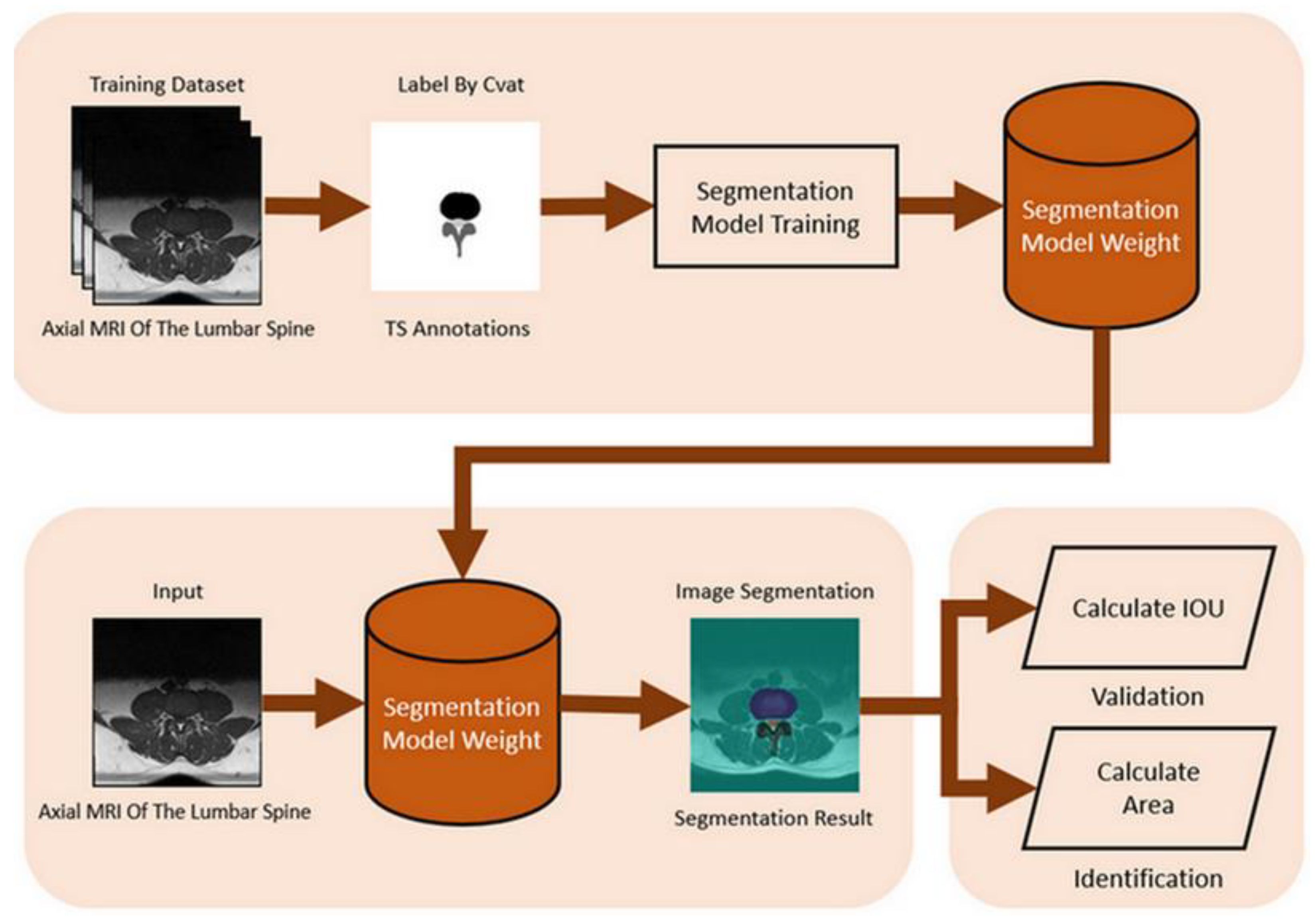
We used the Computer Vision Annotation Tool (CVAT) to label the spinal canal, facet joint, and intervertebral disc in the spinal Magnetic Resonance Imaging (MRI). The marking format is a segmentation mask. The segmentation mask will be used as the ground truth, which is essential for training and validating the spinal canal segmentation model.

For image preprocessing, our study utilizes a spinal canal MRI dataset and manually annotated segmentation masks of the spinal canal area to train this segmentation model. The dataset includes 515 subjects, each with an original spinal canal MRI image and a corresponding ground truth annotation. 300 MRI images were selected for the training dataset, 100 for the test dataset, and the remaining 115 images were the validation dataset.

Libraries such as tensorflow and computer vision were also used. This case needs to identify three portions: the facet joints, intervertebral disc, and spinal canal, so this model hyperparameters are set to width=320 and height=320. Input the image to be tested, apply the trained segmentation model to identify the spinal canal area, and store the recognition result as a segmentation mask. The spinal canal verification and identification of the flowchart is shown in Figure 3.

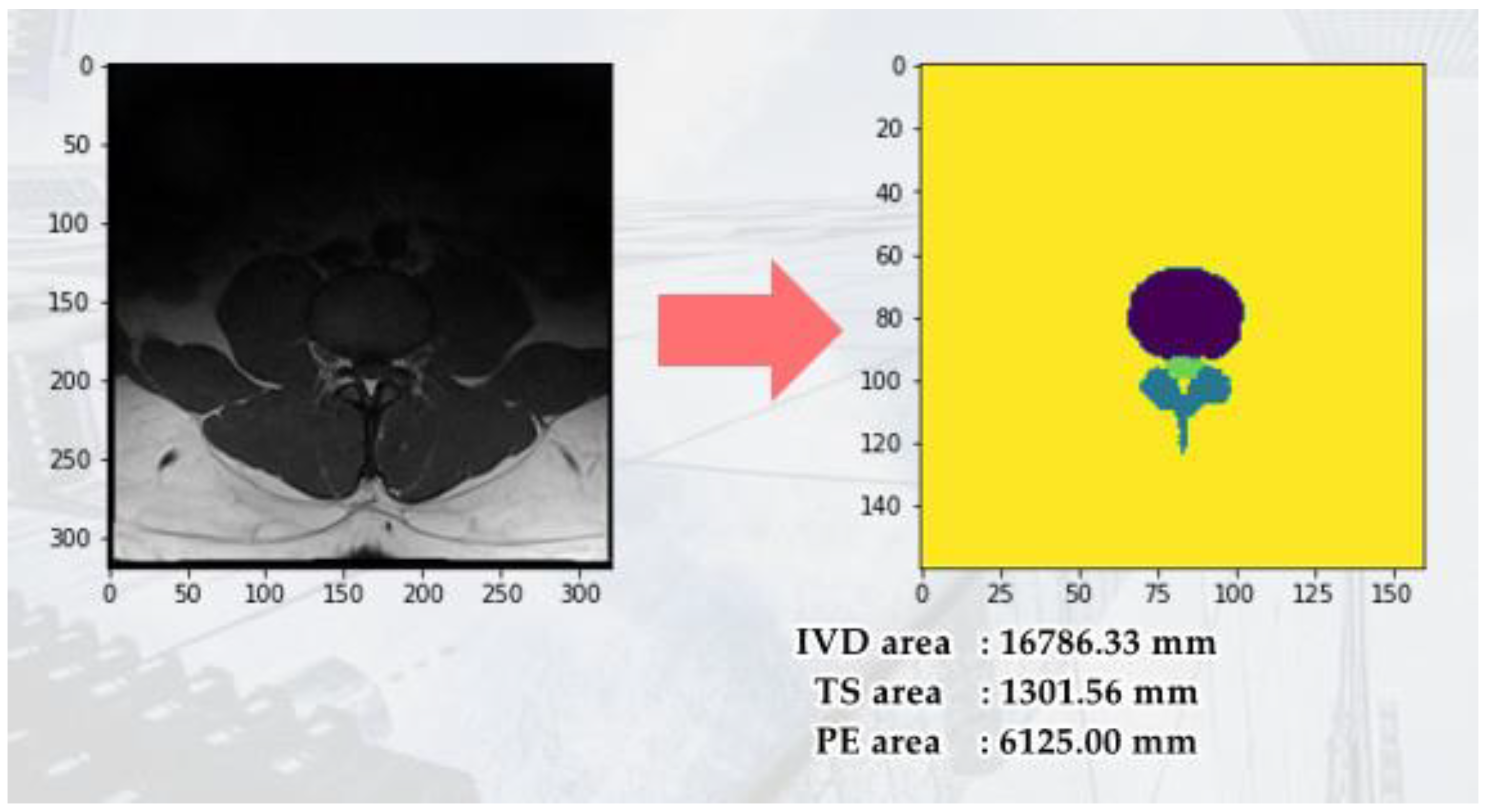
An important parameter of an MRI image is the Field of View (FOV). FOV refers to the imaging range set during an MRI scan, representing the actual length and width of the image. Our study uses the FOV value from the spinal canal MRI image to convert the pixel dimensions in the identification results into actual size (mm²). First, we calculate the number of pixels corresponding to the spinal canal area in the identification result. Then, by multiplying the number of pixels by the genuine size of each pixel, we acquire the cross-sectional area of the spinal canal for the subject. The FOV application to calculate the converted area (mm2) is shown in Figure 4. This approach starts by bring to bear semantic segmentation to the MRI images to identify four regions of interest: The Posterior Element (PE), Intervertebral Disc (IVD), and Thecal Sac (TS).

The labeling work is completed using LabelImg, an image labeling tool that is widely used for object labeling. Image preprocessing for the intervertebral foramen dataset, which includes 40 different subjects, involves handling variations in the aspect size of each MRI image. We resize each image to 416 × 416 pixels to standardize the dataset. Additionally, we apply data augmentation to the dataset. Proper data augmentation helps prevent overfitting during training. Specifically, We enhance the original 80 MRI images by generating an additional 80 images through random rotations, hue adjustments, and brightness modifications.

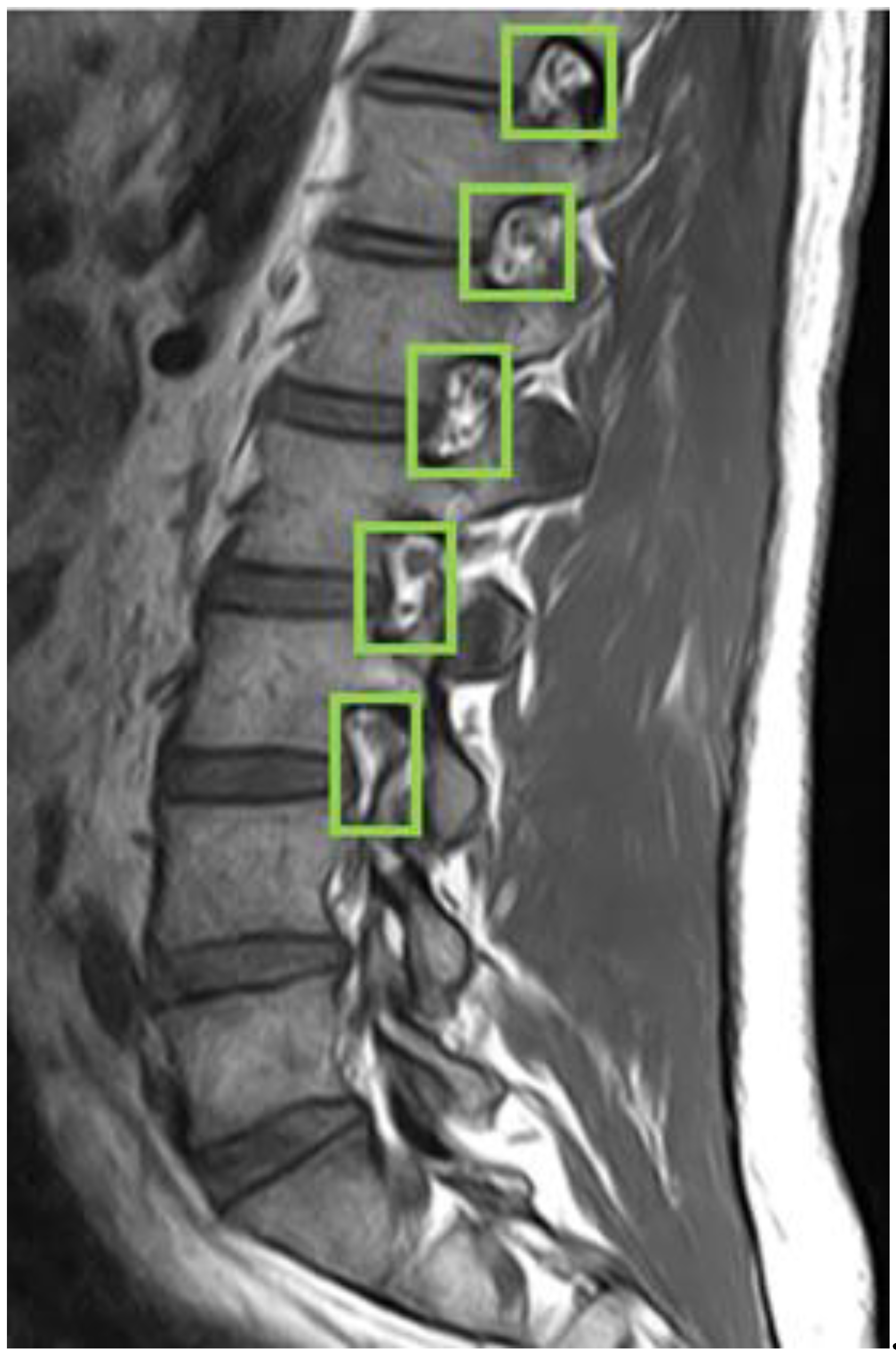
First, we used LabelImg software to delineate the rectangular region of the intervertebral foramen. The annotations were made in YOLO format, with the intervertebral foramen as the sole labeled class. Figure 5 shows an example of a light green-colored annotated intervertebral foramen MRI image.

We allocated 75% of the annotated dataset for training and 25% for validation. The model was trained using YOLOv4 with a batch size of 64, a learning rate of 0.00261, and a maximum of 8,000 batches. YOLO (You Only Look Once) is a one-stage object detection algorithm originally released and developed by Joseph Redmon in 2015. YOLOv4, released in 2020, is known for its speed and high accuracy, making it one of the leading object detection algorithms [19].

This study used CVAT software to annotate the intervertebral foramen in the MRI images, with the annotations in the form of segmentation masks. These segmentation masks serve as the ground truth, essential for training and validating the intervertebral foramen segmentation model.

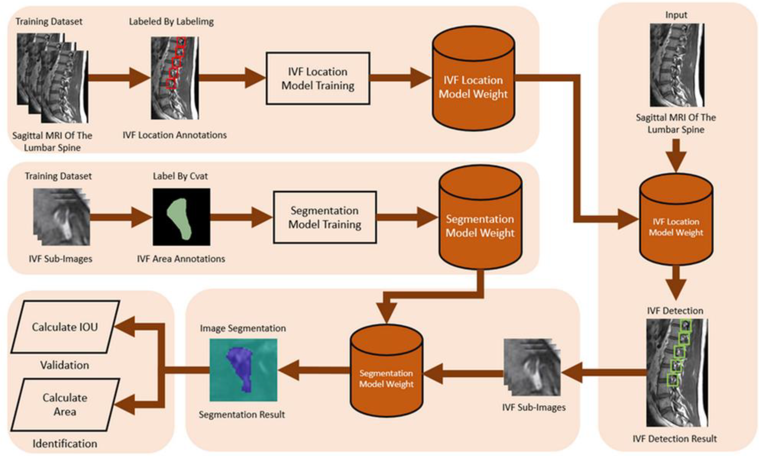
The process of intervertebral foramen object detection begins by inputting the MRI image and using the trained YOLOv4 model to detect the intervertebral foramen within it. Once the intervertebral foramen is identified, the region containing it is cropped into independent rectangular sub-images. These sub-images are then processed using a trained segmentation model to identify the intervertebral foramen area in each one accurately. The recognition results are then stored as segmentation masks.

In morphology, Image Noise is commonly present in the results identified by the segmentation model., which can affect the accuracy of area calculations. To address this, we applied opening and Gaussian blur [24] operations to refine the identified results. We then used the same method to calculate the IOU for the spinal canal to determine the intervertebral foramen IOU, which indicates the model's accuracy. Similarly, we applied the spinal canal area calculation method to determine the intervertebral foramen's actual area, measured in square millimeters (mm²). The flowchart for intervertebral foramen verification and identification is shown in Figure 6.

3. Experimental and Hyperparameter Settings

3.1. Experimental

We used the public spinal canal and intervertebral foramen dataset as the training data in the experiments. The model used a hardware setup featuring a GeForce RTX 2070 WINDFORCE 8G GPU and 32GB of RAM. The software environment consisted of Windows 10 as the operating system, along with Python 3.8 and CUDA 10.2. The hardware experimental environment specification list is shown in Table 1.

3.2. HyperParameter Settings

When training neural networks, adjusting hyperparameters can lead to better results. However, image data labeling is one of the most critical and time-consuming stages in this process, particularly when human resources are limited. In such scenarios, obtaining an immense number of labeled images for training in a short period can be challenging, often resulting in a dataset that is insufficiently sized. Consequently, the time efficiency of data labeling becomes an important issue.

To solve this problem, we employed data augmentation techniques in our research. This approach allows us to generate numerous variant images from a limited set of labeled images, effectively expanding the training dataset without incurring additional manual labeling costs. This method improves the efficiency of data labeling and enhances the model's learning capability and generalization performance. The YOLOv4[19] hyperparameter setup is shown in Table 2.

3.3. Evaluation Metrics

Intersection over Union (IoU)is a standard metric used to measure the accuracy of detecting corresponding objects within a specific dataset. The IoU indicator will help us fully understand the model's relevance and guide us to further optimization. IoU is computed by dividing the intersection of the predicted result with the ground truth by their union.

I o U = \frac{a r e a (A \cap B)}{a r e a (A \cup B)}

(2)

In the formulas, True Positives (TP) refers to the number of objects correctly identified, False Positives (FP) denotes the number of objects incorrectly identified as belonging to a different class, and False Negatives (FN) represents the number of objects from the target class that were incorrectly classified as belonging to another class. Therefore, TP+FP represents the total number of objects predicted by the model, while TP+FN represents the actual number of objects in the target class.

The average precision (AP) was used to evaluate the proposed method's model detection and segmentation performance. All the AP values of all categories were also averaged to output mean Average Precision (mAP). The calculation Formula (3) for mAP is as follows:

m A P = \frac{\sum_{n = 1}^{N} {A P}_{n}}{N}

(3)

4. Results

4.1. Spinal Canal Identification

4.1.1. Training Different Segmentation Models Based on Image Category

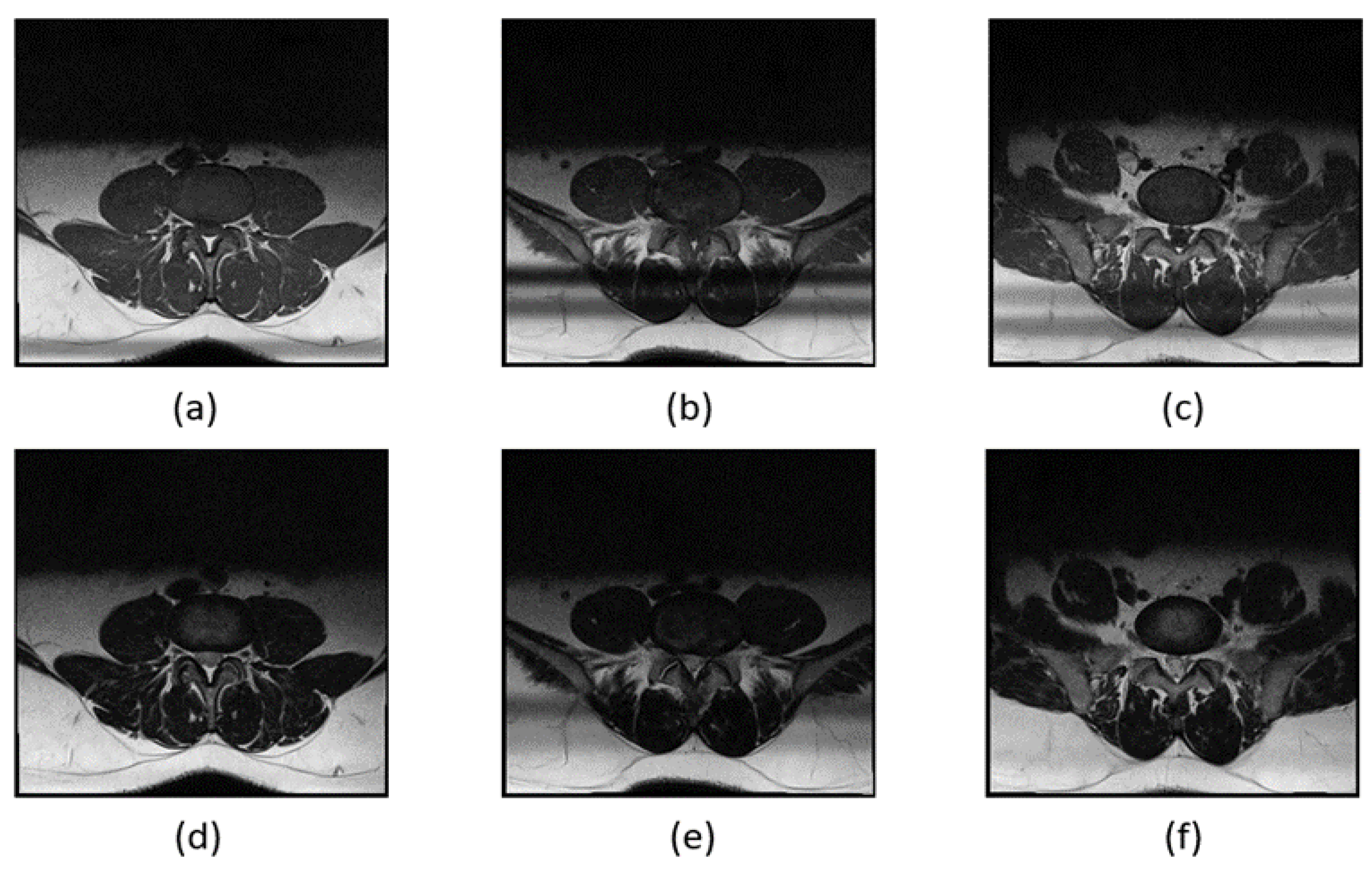
The MRI images of the subject's spinal canal include D3, D4, and D5, with each section imaged using two weighting methods, T1 and T2, resulting in a total of six images. The spinal canal, intervertebral discs, and facet joints differ slightly in shape and size across these six images. To prevent these differences from affecting segmentation performance, we trained separate segmentation models for each MRI image of the spinal canal. This approach aims to minimize the impact of variations between different images on segmentation accuracy.

Noticeable differences between the images (a) and (f). In the MRI images of L3 and L4, the facet joints of the spinal canal are more pronounced, while the L5 segment is connected to the S1 segment, giving the spinal canal a distinct shape. T1 and T2 weighting also have a significant impact on the image appearance. T1 weighting enhances the fat tissues in the MRI image, making the spinal canal appear entirely black, whereas T2 weighting highlights the watery tissues, resulting in a lighter spinal canal where some white nerves are visible. The spinal canal in different sections using T1 and T2 weighting is illustrated in Figure 7.

4.2. Model Comparison

We utilized ResNet50 and VGG16 as the encoding architectures, combined with U-Net and SegNet[25] as the decoding architectures, to form four segmentation models: VGG_U-Net, VGG_SegNet, ResNet_SegNet, and ResNet_U-Net. The performance of these models was evaluated using the mean Intersection over Union (IOU) and the standard deviation of IOU (IOU Std) as metrics. The model with the highest mean IOU and the lowest IOU Std was selected as the best segmentation model.

This compares the mean IOU and IOU standard deviation of the four segmentation models: VGG_U-Net, VGG_SegNet, ResNet_U-Net, and ResNet_SegNet. Among them, ResNet_U-Net has the best performance. Overall, it can be found that Resnet50 performs better than VGG16 in the case of the spinal canal. A comprehensive comparison is shown in Table 3.

4.3. Intervertebral Foramen Identification

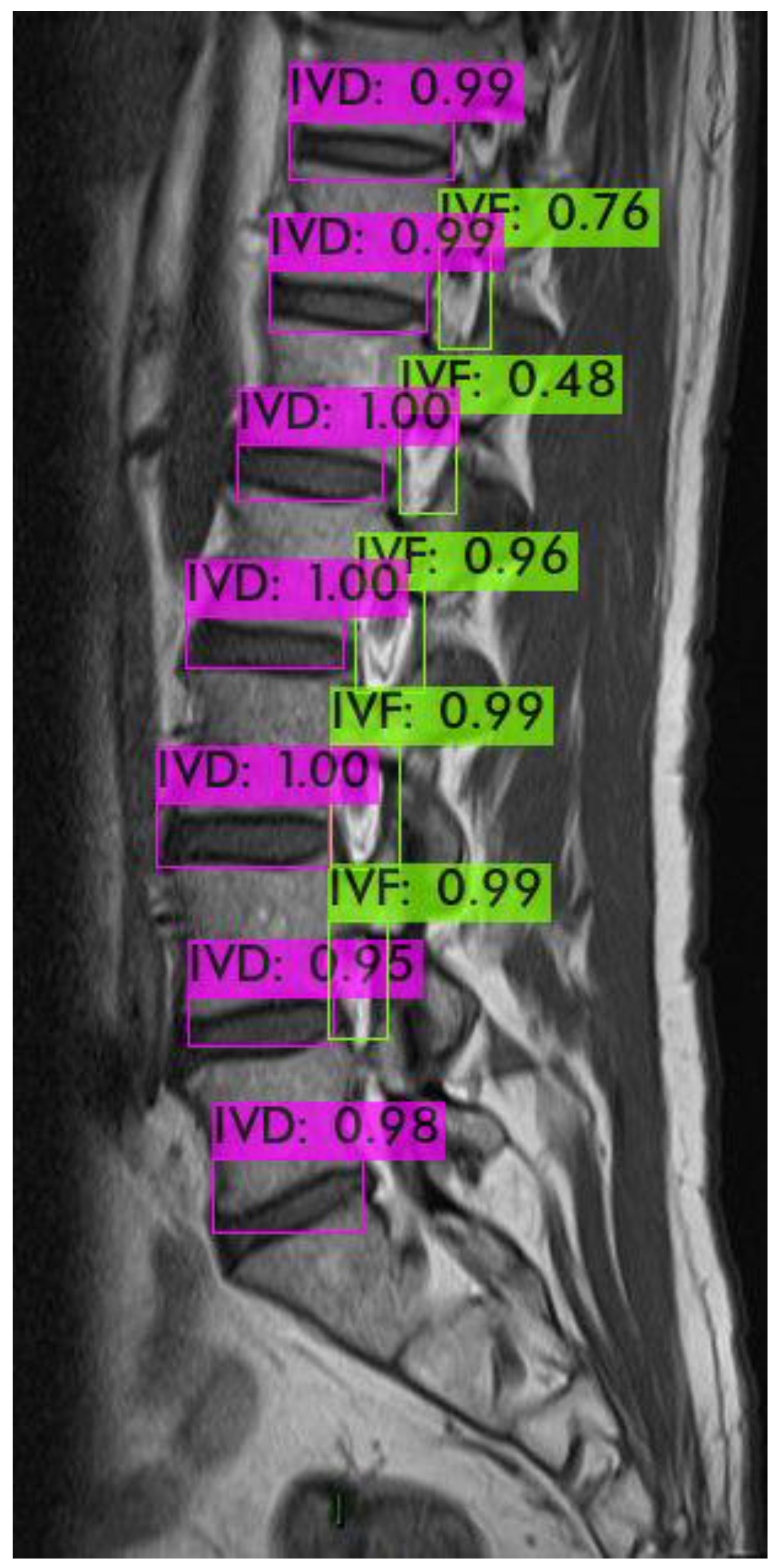
For identifying the area of the intervertebral foramen (IVF) and intervertebral disc (IVD), we first employ the YOLOv4 object detection model to detect the intervertebral foramen in MRI images shown in Figure 8. The detected foramen is then cropped into sub-images, which are further processed using DL methods to segment the areas of the IVF and IVD within these sub-images. After segmentation, the number of pixels occupied by the intervertebral foramen in the MRI dataset is analyzed. Finally, by using the Field of View (FOV), detailed information from the MRI dataset, this pixel count is converted into an actual area measurement in square millimeters.

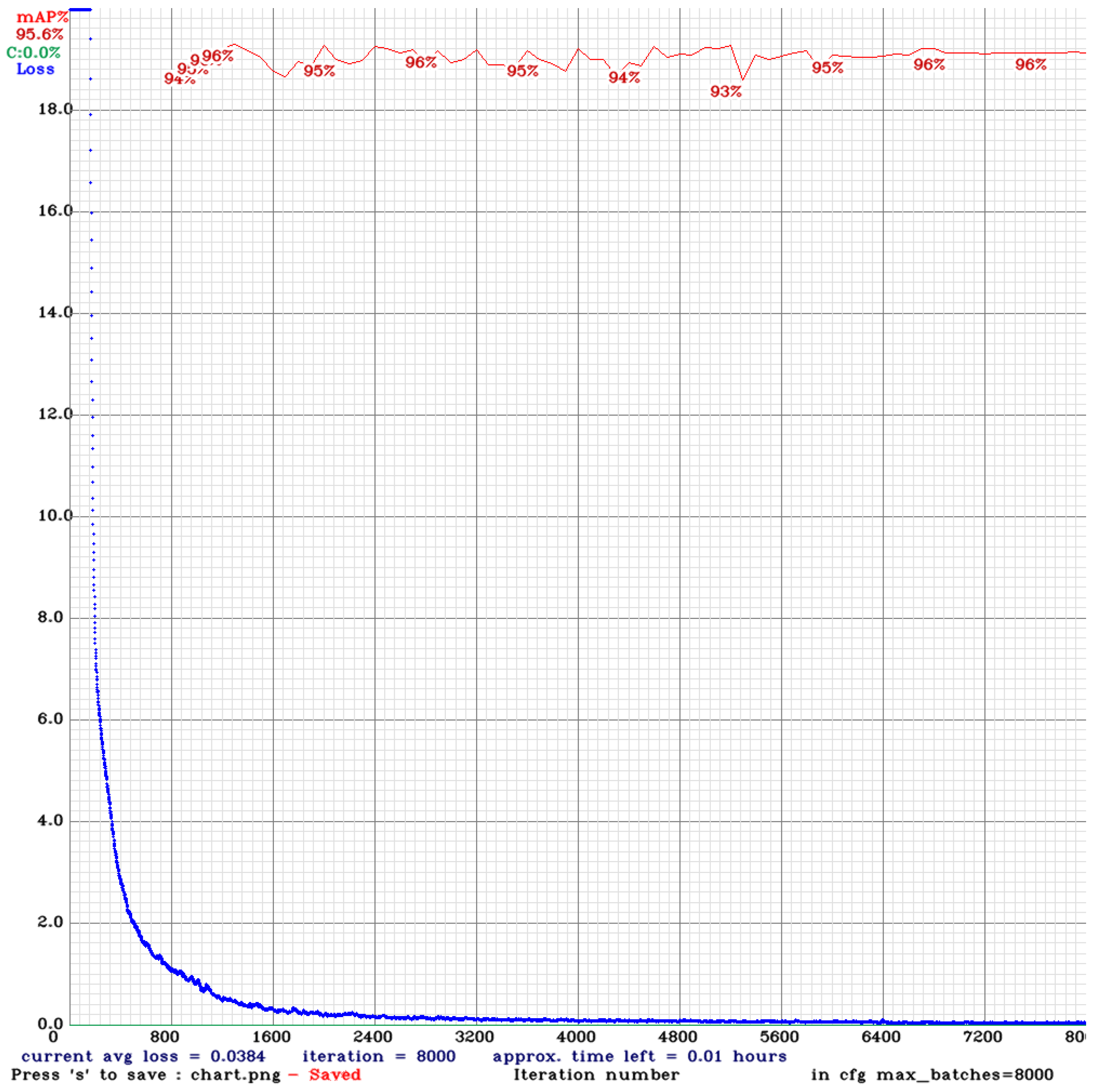
The experiment reveals that during the training process of the model using YOLOv4, various performance indicators are displayed, including the changes in loss and mean Average Precision (mAP). The following is an analysis of the training process: The blue line (Loss) represents the model's loss value during training. Initially, the loss value decreases rapidly, indicating that the model learns features from the images effectively. As the number of iterations rises, the loss of numerical value continues to decrease steadily and gradually stabilizes.

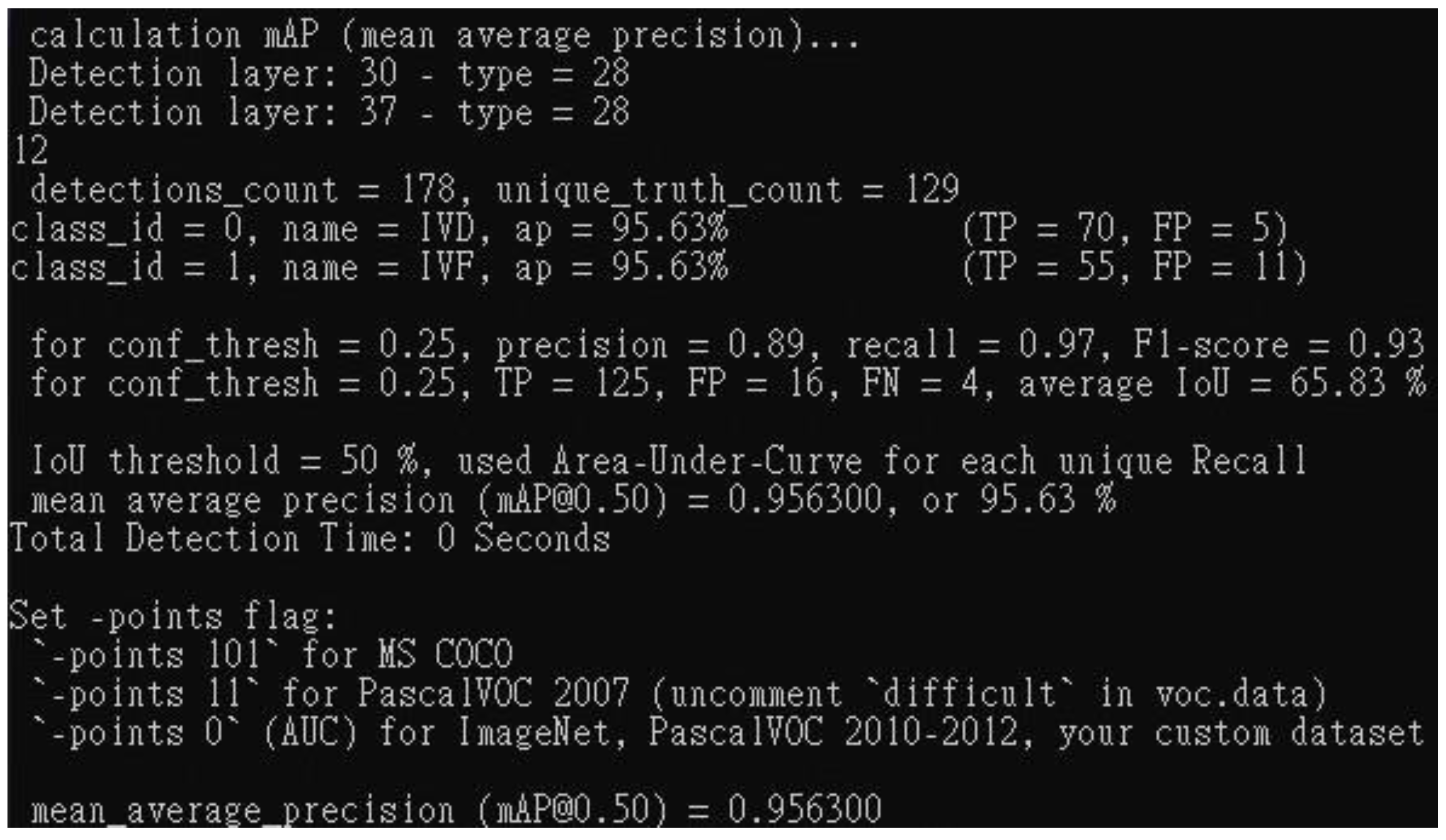
As shown in Figure 9 about the YOLOv4 Training process, the initial mAP value is 94%. As the number of training iterations elevates, the loss diminishes, and the mAP rises, reaching a maximum of 96%, around 1,300 iterations. However, as training continues, overfitting begins to occur, where the model becomes overly specialized to the training image dataset, making it challenging to predict or differentiate new, unseen data accurately. This leads to a slight decrease in mAP. Despite this, the mAP value stabilized at 96% between 6,000 and 8,000 iterations, with the final mAP recorded at 95.6%. YOLOv4 training result is shown in Figure 10.

4.4. Assessment of Models and Morphological Processing Techniques

Similarly, to the comparison of different models for spinal canal identification, we employed VGG16 and ResNet50 as the encoding architectures and U-Net and SegNet as the decoding architectures, forming four segmentation models: VGG_U-Net, VGG_SegNet, ResNet_U-Net, and ResNet_SegNet. We evaluated the performance of these models using the mean IOU and IOU standard deviation (IOU Std) indicators. The model with the highest average IoU and the lowest IoU standard deviation was selected as the best segmentation model based on the experimental results.

The ResNet50-U-Net model achieved the highest IOU mean value and the lowest IOU Std value. Table 4 compares the IOU mean and IOU Std values of the four segmentation models—VGG_U-Net, VGG_SegNet, ResNet50_U-Net, and ResNet_SegNet—after applying morphology processing. The identification results are consistent with those in Table 5. It can be observed that after applying morphology processing, the IOU mean for VGG_U-Net and ResNet50-U-Net, which use U-Net as the decoding model, improved, while the IOU Std remained largely unaffected. Conversely, the IOU mean for VGG_SegNet and ResNet50_SegNet, which use SegNet as the decoding model, decreased, along with a reduction in IOU Std.

5. Discussion

With increasing age in the population, the incidence of spinal stenosis is expected to slowly increase, with approximately 266 million population suffering from lumbar degenerative diseases each year. This trend underscores the growing importance of developing quick, convenient, and standardized methods for detecting spinal stenosis, which has emerged as a key challenge in the medical realm.

Earlier investigations have utilized deep learning techniques to identify spinal stenosis, their indicators often lack precision, relying on coarse metrics such as four-point scales or dichotomous classifications to represent severity. In this study, we first used YOLO to locate intervertebral discs (IVD) and intervertebral foramina (IVF) and then utilized the area as more refined indicators to assess spinal stenosis. Our approach significantly achieves the 95.6 % mean average precision (mAP) of detection.

Using areas as indices for assessing spinal stenosis enhances patients' understanding of symptom severity and facilitates hospital data collection and standardization. On top of that, by introducing new models and indicators, this paper found that applying dilation and erosion skills to address image noise produced precise image results. The two models, Resnet50 mixing U-Net, that we employed to discern the spinal canal and intervertebral foramen, achieved IoU scores of 79.11 and 80.89, respectively, indicating reliable performance. Although there is still some way to match mature object recognition models, this study has established a precedent for using areas as indicators in assessing spinal stenosis.

Looking ahead, more reliable indicators or models can be developed, and code for identifying MRI images can be released. The concepts and models proposed in this paper could be adapted to imaging other anatomical regions.

In conclusion, spinal canal MRI images are captured using two weighting methods, T1 and T2, across three sections, L3, L4, and L5, resulting in six images. The segmentation model was trained separately for each spinal canal MRI image, with the ResNet50-U-Net model demonstrating the best performance, achieving an IoU as high as 80.89% (noting that the standard benchmark for a reasonable recognition rate is an IoU of 0.5 or higher). Overall, the results indicate that ResNet50 outperforms VGG16 in spinal canal identification.

To identify the intervertebral foramen area, we will compare the results obtained with and without erosion and dilation processing and evaluate the influence of these image-processing techniques on the identification outcomes. Among the approaches that exclude erosion and dilation, the ResNet50-U-Net model demonstrates the best performance. Using U-Net as the decoding model improves the IOU mean for intervertebral foramen identification when applying morphological processing.

6. Conclusions

Our study is the first to use deep learning mixed with computer vision to identify spinal stenosis, using Intersection over Union (IoU) and mean Average Precision (mAP) as verification indicators. The approach involves segmenting the relevant anatomical structures and then calculating their areas. Unlike previous studies that categorized symptoms into broad two-part or four-part classifications, this research provides a more explicit and objective assessment of the degree of spinal stenosis. Additionally, by employing techniques such as morphological processing, the study significantly improves the average IoU and mAP for intervertebral foramen identification.

Author Contributions

C.Y.W conceived the paper direction, study for literature, C.W.H conceived the experiments and analyzed the results, Z.J.L conducted the method and material part, S.M.C., C.W.H., Z.J.L. assisted the experiments. All authors reviewed the manuscript.

Institutional Review Board Statement

All procedures performed in studies involving human participants were in accordance with the ethical standards of the institutional and/or national research committee. The information in this paper comes from public datasets, no ethical issues.

Informed Consent Statement

Not applicable.

Data Availability Statement

Data supporting this study are openly available from Radiopaedia at https://radiopaedia.org/?lang=us and Lumbar Spine MRI Dataset at https://data.mendeley.com/datasets/k57fr854j2/2.

Acknowledgments

Thanks Sud Sudirman, Ala Al Kafri, Friska Natalia, Hira Meidia, Nunik Afriliana, Wasfi Al-Rashdan, Mohammad Bashtawi, Mohammed Al-Jumaily for their dataset. Thanks Alexey Bochkovskiy, Chien-Yao Wang, Hong-Yuan Mark Liao for making yolov4 public. Thanks JohnAshburnerKarl J. Friston for making segmentation public.

Conflicts of Interest

All authors have and declare that: (i) no support, financial or otherwise, has been received from any organization that may have an interest in the submitted work; and (ii) there are no other relationships or activities that could appear to have influenced the submitted work.

References

Berry, K.P.; Nedivi, E. Spine dynamics: Are they all the same? Neuron 2017, 96, 43–55. [Google Scholar] [CrossRef] [PubMed]
Ravindra, V.M.; Senglaub, S.S.; Rattani, A.; Dewan, M.C.; Härtl, R.; Bisson, E.; Park, K.B.; Shrime, M.G. Degenerative lumbar spine disease: Estimating global incidence and worldwide volume. Global spine journal 2018, 8, 784–794. [Google Scholar] [CrossRef] [PubMed]
Kos, N.; Gradisnik, L.; Velnar, T. A brief review of the degenerative intervertebral disc disease. Medical Archives 2019, 73, 421. [Google Scholar] [CrossRef] [PubMed]
Boden, S.D.; Davis, D.; Dina, T.; Patronas, N.; Wiesel, S. Abnormal magnetic-resonance scans of the lumbar spine in asymptomatic subjects. A prospective investigation. JBJS 1990, 72, 403–408. [Google Scholar] [CrossRef]
Kaul, V.; Enslin, S.; Gross, S.A. History of artificial intelligence in medicine. Gastrointestinal endoscopy 2020, 92, 807–812. [Google Scholar] [CrossRef] [PubMed]
Kulkarni, S.; Seneviratne, N.; Baig, M.S.; Khan, A.H.A. Artificial intelligence in medicine: Where are we now? Academic radiology 2020, 27, 62–70. [Google Scholar] [CrossRef] [PubMed]
Liu, P.-r.; Lu, L.; Zhang, J.-y.; Huo, T.-t.; Liu, S.-x.; Ye, Z.-w. Application of artificial intelligence in medicine: An overview. Current medical science 2021, 41, 1105–1115. [Google Scholar] [CrossRef] [PubMed]
Azimi, P.; Yazdanian, T.; Benzel, E.C.; Aghaei, H.N.; Azhari, S.; Sadeghi, S.; Montazeri, A. A review on the use of artificial intelligence in spinal diseases. Asian Spine Journal 2020, 14, 543. [Google Scholar] [CrossRef] [PubMed]
Hallinan, J.T.P.D.; Zhu, L.; Yang, K.; Makmur, A.; Algazwi, D.A.R.; Thian, Y.L.; Lau, S.; Choo, Y.S.; Eide, S.E.; Yap, Q.V. Deep learning model for automated detection and classification of central canal, lateral recess, and neural foraminal stenosis at lumbar spine MRI. Radiology 2021, 300, 130–138. [Google Scholar] [CrossRef] [PubMed]
Lewandrowski, K.-U.; Muraleedharan, N.; Eddy, S.A.; Sobti, V.; Reece, B.D.; León, J.F.R.; Shah, S. Artificial intelligence comparison of the radiologist report with endoscopic predictors of successful transforaminal decompression for painful conditions of the lumber spine: Application of deep learning algorithm interpretation of routine lumbar magnetic resonance imaging scan. International journal of spine surgery 2020, 14, S75–S85. [Google Scholar] [PubMed]
Rak, M.; Tönnies, K.D. On computerized methods for spine analysis in MRI: A systematic review. International journal of computer assisted radiology and surgery 2016, 11, 1445–1465. [Google Scholar] [CrossRef] [PubMed]
Dongare, A.; Kharde, R.; Kachare, A.D. Introduction to artificial neural network. International Journal of Engineering and Innovative Technology (IJEIT) 2012, 2, 189–194. [Google Scholar]
He, K.; Zhang, X.; Ren, S.; Sun, J. Deep residual learning for image recognition. In Proceedings of Proceedings of the IEEE conference on computer vision and pattern recognition; pp. 770–778.
Simonyan, K.; Zisserman, A. Very deep convolutional networks for large-scale image recognition. arXiv 2014, arXiv:1409.1556. [Google Scholar]
Krizhevsky, A.; Sutskever, I.; Hinton, G.E. Imagenet classification with deep convolutional neural networks. Advances in neural information processing systems 2012, 25. [Google Scholar] [CrossRef]
Szegedy, C.; Liu, W.; Jia, Y.; Sermanet, P.; Reed, S.; Anguelov, D.; Erhan, D.; Vanhoucke, V.; Rabinovich, A. Going deeper with convolutions. In Proceedings of Proceedings of the IEEE conference on computer vision and pattern recognition; pp. 1–9.
Ronneberger, O.; Fischer, P.; Brox, T. U-net: Convolutional networks for biomedical image segmentation. Proceedings of Medical image computing and computer-assisted intervention–MICCAI 2015: 18th international conference, Munich, Germany, 2015, proceedings, part III 18, October 5-9; pp. 234–241.
Bank, D.; Koenigstein, N.; Giryes, R. Autoencoders. Machine learning for data science handbook, 2023. [Google Scholar]
Bochkovskiy, A.; Wang, C.-Y.; Liao, H.-Y.M. Yolov4: Optimal speed and accuracy of object detection. arXiv 2020, arXiv:2004.10934. [Google Scholar]
Natalia, F.; Meidia, H.; Afriliana, N.; Al-Kafri, A.S.; Sudirman, S.; Simpson, A.; Sophian, A.; Al-Jumaily, M.; Al-Rashdan, W.; Bashtawi, M. Development of ground truth data for automatic lumbar spine MRI image segmentation. Proceedings of 2018 IEEE 20th International Conference on High Performance Computing and Communications; IEEE 16th International Conference on Smart City; IEEE 4th International Conference on Data Science and Systems (HPCC/SmartCity/DSS); pp. 1449–1454.
Al-Kafri, A.S.; Sudirman, S.; Hussain, A.; Al-Jumeily, D.; Natalia, F.; Meidia, H.; Afriliana, N.; Al-Rashdan, W.; Bashtawi, M.; Al-Jumaily, M. Boundary delineation of MRI images for lumbar spinal stenosis detection through semantic segmentation using deep neural networks. IEEE Access 2019, 7, 43487–43501. [Google Scholar] [CrossRef]
I, B. Bickle I, Normal lumbar spine MRI. Case study, Radiopaedia.org. Availabe online: https://radiopaedia.org/cases/47857. (accessed on 7 September 2016).
Muzio, B.D. Normal lumbar spine MRI - low-field MRI scanner. Case study, Radiopaedia.org. Availabe online: https://radiopaedia.org/cases/40976. (accessed on 10 November 2015).
Hummel, R.A.; Kimia, B.; Zucker, S.W. Deblurring gaussian blur. Computer Vision, Graphics, and Image Processing 1987, 38, 66–80. [Google Scholar] [CrossRef]
Badrinarayanan, V.; Kendall, A.; Cipolla, R. Segnet: A deep convolutional encoder-decoder architecture for image segmentation. IEEE transactions on pattern analysis and machine intelligence 2017, 39, 2481–2495. [Google Scholar] [CrossRef] [PubMed]

Figure 1. U-net architecture [17].

Figure 2. autoencoder model[18].

Figure 3. YOLO process diagram [19].

Figure 3. The flowchart of spinal canal verification and identification.

Figure 4. Use FOV to calculate the converted area (mm2).

Figure 5. Use LabelImg tool to annotate intervertebral foramen MRI image.

Figure 6. The flowchart for intervertebral foramen verification and identification.

Figure 7. spinal canal in different parts in T1-T2.

Figure 8. YOLOv4 object detection.

Figure 9. YOLOv4 Training process.

Figure 10. YOLOv4 training result.

Table 1. Hardware experimental environment specification list.

Table 2. YOLOv4 hyperparameters setup.

Table 3. The comparison of different model's IOU mean and IOU Std value.

S.No	Encode Model	Decode Model	IOU mean	IOU Std
1	VGG16	Unet	73.94	9.54
2	VGG16	Segnet	66.94	10.38
3	Resnet50	Unet	77.4	8.77
4	Resnet50	Segnet	68.61	12.58

Table 4. This table represents the comparison of different model's IOU mean and IOU Std value.

S.No	Encode Model	Decode Model	IOU mean	IOU Std
1	VGG16	U-Net	61.19	10.85
2	VGG16	Segnet	48.11	12.28
3	Resnet50	U-Net	79.11	9.40
4	Resnet50	Segnet	50.47	14.42

Table 5. This table represents the comparison of different model's IOU mean and IOU Std value.

S.No	Encode Model	Decode Model	IOU mean	IOU Std
1	VGG16	U-Net	64.97	10.85
2	VGG16	Segnet	45.26	8.99
3	Resnet50	U-Net	80.89	9.44
4	Resnet50	Segnet	43.09	10.60

Disclaimer/Publisher’s Note: The statements, opinions and data contained in all publications are solely those of the individual author(s) and contributor(s) and not of MDPI and/or the editor(s). MDPI and/or the editor(s) disclaim responsibility for any injury to people or property resulting from any ideas, methods, instructions or products referred to in the content.

© 2024 by the authors. Licensee MDPI, Basel, Switzerland. This article is an open access article distributed under the terms and conditions of the Creative Commons Attribution (CC BY) license (https://creativecommons.org/licenses/by/4.0/).

Copyright: This open access article is published under a Creative Commons CC BY 4.0 license, which permit the free download, distribution, and reuse, provided that the author and preprint are cited in any reuse.

Alerts

MDPI Initiatives

Important Links

Choose an area of interest and we will send you notifications of new preprints at your preferred frequency.

Disclaimer