
Submitted:
04 September 2024
Posted:
04 September 2024
You are already at the latest version
Abstract
This paper presents an advanced software tool for precise laser beam propagation analysis, focusing on the calculation of the M2 value, a key measure of beam quality. Developed in Python, the software integrates libraries like NumPy, Matplotlib, and SciPy for robust data handling and accurate polynomial fitting. It features a user-friendly interface for easy data input, analysis, and visualization, making it accessible to both professionals and novices. The tool has been rigorously validated against theoretical models (M2=1) and experimental data (showing M2=1.2548 and 1.3166), ensuring high accuracy and reliability. It visualizes beam width data and fitted polynomial curves, aiding in assessing beam propagation characteristics and optimizing laser systems. Future enhancements include additional beam quality metrics, machine learning integration, and cloud-based functionality. This tool significantly advances laser beam analysis, benefiting research and industrial applications by improving performance and efficiency. The software is available at DOI: 10.5281/zenodo.13325911
Keywords:
Laser beam
; Propagation analysis
; Python
; Polynomial fitting
; Beam quality factor
; Software
1. Introduction
Laser beam propagation analysis is a vital component in numerous scientific and industrial applications [1]. Understanding and controlling the behaviour of laser beams is essential for optimizing performance in areas such as material processing, medical treatments, and communication technologies. One of the key parameters in evaluating beam quality is the M2 value, which serves as an indicator of the focusability and overall efficiency of a laser. An accurate determination of this value is critical to ensuring the effectiveness and precision of laser systems [2].
Traditionally, calculating the M2 value has been a complex and labour intensive task [3,4,5]. Researchers and engineers often rely on intricate experimental setups and extensive data analysis to derive this parameter. These methods, while accurate, can be cumbersome and time-consuming, requiring significant expertise and resources [6,7,8]. The need for a more streamlined approach to M2 value calculation has become increasingly apparent, especially as the demand for high-performance laser applications continues to grow.
In response to this need, this paper presents a novel software tool designed to simplify the process of M2 value determination. By employing advanced polynomial fitting techniques, the software offers a more efficient and user-friendly alternative to traditional methods. The tool not only automates the calculation process, but also improves accuracy and reliability, reducing the potential for human error and expediting the analysis workflow.
In addition, the software features an intuitive graphical user interface (GUI) that allows users to easily interact with the system and visualize results. This interface is designed to be accessible to both experienced professionals and those new to laser beam analysis, ensuring that a wide range of users can benefit from its capabilities. By integrating these innovative features, the software stands to significantly impact the field of laser beam propagation analysis, providing a valuable resource for improving the performance and efficiency of laser systems across various applications.
2. Methodology
2.1. Development and Architecture of the Software
The software designed for simplifying the calculation of the M2 value was developed using Python [9], a powerful and versatile programming language known for its ease of use and robust libraries. The development process involved integrating several essential libraries, including NumPy, Matplotlib, and SciPy, to achieve the desired functionality and performance [10].
2.1.1. Key Libraries and Their Roles
NumPy
This library is fundamental for numerical computations in Python. It provides support for arrays, matrices, and high-level mathematical functions. In our software, NumPy is utilized to handle large datasets of beam width measurements efficiently and perform necessary mathematical operations, such as polynomial fitting.
Matplotlib
Visualization is a critical aspect of data analysis and interpretation. Matplotlib is a comprehensive library for creating static, animated, and interactive visualizations in Python. In this software, Matplotlib is used to plot the beam width data and the fitted polynomial curve, allowing users to visually inspect the accuracy of the fit and the quality of the laser beam.
SciPy
This library builds on NumPy and provides additional functionality for scientific and technical computing. SciPy’s optimization and curve fitting modules are particularly important for this software. They enable the precise fitting of the squared beam width data to a second-order polynomial, which is essential for accurate M2 value calculation.
2.2. Primary Functionality
The core functionality of the software revolves around fitting the squared beam width data to a second-order polynomial and calculating the M2 value based on the fitted parameters. This process can be broken down into several key steps:
2.2.1. Data Input and Preprocessing
The software allows users to input beam width measurements obtained from laser propagation experiments. These measurements typically consist of the beam width at various points along the propagation axis. The software preprocesses this data to ensure it is in the correct format for analysis.
2.2.2. Polynomial Fitting
Using the SciPy library, the software fits the squared beam width data to a second-order polynomial. This involves finding the polynomial coefficients that best describe the relationship between the beam width and the propagation distance. The fitting process minimizes the difference between the observed data points and the values predicted by the polynomial model.
2.2.3. M2 Calculation
Once the polynomial coefficients are obtained, the software calculates the M2 value. The M2 value is a measure of the beam quality and is derived from the coefficients of the fitted polynomial. Specifically, it is calculated based on the ratio of the divergence of the beam to the divergence of an ideal Gaussian beam [11].
2.2.4. Visualization
The software uses Matplotlib to generate plots that display the original beam width data and the fitted polynomial curve. These visualizations provide users with a clear understanding of the fit’s accuracy and the beam’s propagation characteristics.
2.2.5. User Interface
The graphical user interface (GUI) of the software is designed to be intuitive and user-friendly. It allows users to easily input data, run the analysis, and view results. The GUI provides controls for adjusting parameters, selecting data files, and customizing the visualizations.
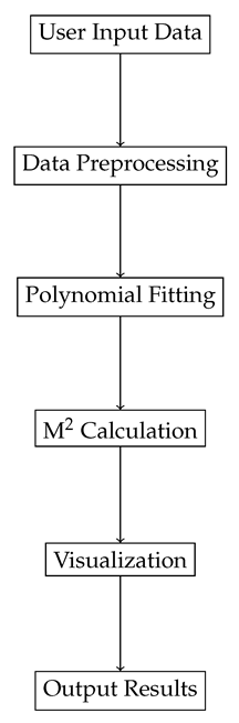
2.3. Software Workflow Diagram
Below is a diagram illustrating the workflow of the software:
2.4. Example Analysis
To illustrate the functionality of the software, let’s consider an example analysis:
2.4.1. Input Data
The user inputs beam width measurements at various propagation distances. These measurements are stored in an array format, where each element represents the beam width at a specific distance.
2.4.2. Data Preprocessing
The software preprocesses the input data by squaring the beam width values. This step is necessary for fitting the data to a second-order polynomial.
2.4.3. Polynomial Fitting
Using the SciPy library, the software fits the squared beam width data to a second-order polynomial. The fitting process involves solving an optimization problem to find the polynomial coefficients that minimize the error between the observed data and the polynomial model.
2.4.4. M2 Calculation
With the polynomial coefficients obtained, the software calculates the M2 value. This involves computing the ratio of the beam’s divergence to the divergence of an ideal Gaussian beam, based on the polynomial coefficients.
Theoretically, the beam quality factor [12], , is a measure of how close a laser beam is to an ideal Gaussian beam. For a perfect Gaussian beam, . For real laser beams, is greater than 1, indicating deviations from the ideal Gaussian profile.
The factor is defined using the following theoretical relationships: Beam Waist (): The beam waist is the location where the beam diameter reaches its minimum value. Rayleigh Range (): The Rayleigh range is the distance over which the beam remains approximately collimated and is given by:
where is the wavelength of the laser.
Beam Divergence Angle : The far-field divergence of the beam is defined as:
Propagation Factor (): The beam quality factor is defined by comparing the divergence of the actual beam to that of an ideal Gaussian beam:
Simplifying the relationship:
General Expression for : The beam radius at a distance z from the beam waist can be described as:
where is the beam radius at distance z from the beam waist.
2.4.5. Visualization
The software generates a plot that displays the original beam width data and the fitted polynomial curve. This plot provides a visual representation of the beam’s propagation characteristics and the accuracy of the polynomial fit.
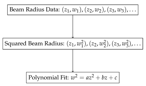
2.5. Polynomial Fitting Example Diagram
Below is a diagram illustrating the polynomial fitting process:
2.6. Benefits and Impact
The software provides several significant benefits over traditional methods of M2 value calculation:
2.6.1. Efficiency
The software automates the calculation process, significantly reducing the time and effort required for analysis. This allows researchers and engineers to focus on interpreting results and optimizing laser systems.
2.6.2. Accuracy
By leveraging advanced polynomial fitting techniques, the software ensures accurate and reliable M2 value calculations. This improves the precision of beam quality assessments and enhances the performance of laser applications.
2.6.3. User-Friendly Interface
The intuitive GUI makes the software accessible to a wide range of users, from experienced professionals to those new to laser beam analysis. The interface simplifies data input, analysis, and visualization, providing a seamless user experience.
2.6.4. Visualization
The ability to visualize the beam width data and the fitted polynomial curve helps users understand the propagation characteristics of the laser beam. This visual feedback is invaluable for assessing the quality of the fit and making informed decisions about laser system optimization.
3. Results
The software was evaluated using a variety of datasets, encompassing different sets of propagation distances and beam radius, to thoroughly test its accuracy and reliability in calculating the M2 value. The primary goal of this evaluation was to compare the results produced by the software with established theoretical models (M2 = 1 for perfect Gaussian), thereby validating its performance.
3.1. Evaluation Process
The evaluation process involved the following steps:
- Data Collection: Various sets of beam radius measurements were obtained from controlled laser propagation experiments. These measurements included beam radiuses recorded at multiple propagation distances using a CCD camera, ensuring a comprehensive data set for analysis.
- Data Input: The data collected were then inputted into the software. The preprocessing capabilities of the software ensured that the data were correctly formatted and ready for analysis.
- Polynomial Fitting: Using its advanced polynomial fitting algorithms, the software processed the squared beam width data to generate second-order polynomial fits.
- M2 Calculation: Based on the polynomial fits, the software calculated the M2 values, providing a measure of the beam quality.
3.2. Data Collected
The data collected from the laser propagation experiments are shown in Table 1.
3.3. Visual Representation of Results
Figure 1 and Figure 2 present examples of the squared beam width data plotted against propagation distance, accompanied by the corresponding polynomial fits. These visualizations are crucial for understanding the software’s ability to accurately model beam width data through polynomial fitting techniques.
In Figure 1, the squared beam width data points (second moment) are shown along with a polynomial curve that fits the data. The second moment width, also known as D4, is a measure of the spatial profile of the beam. It is calculated from the intensity distribution of the beam and involves integrating the entire beam profile. This method provides a comprehensive measure of the beam’s width, accounting for the entire spatial distribution of the light intensity. The close alignment of the data points with the polynomial fit indicates that the software accurately models the beam width data. This alignment is critical to ensure that the M2 value derived from these fits is reliable.
Similarly, Figure 2 displays another data set (knife edge) where the squared beam width is plotted against the propagation distance. The knife-edge method measures the beam width by moving a knife-edge across the beam and recording the power of the light passing by the edge. The beam width is then determined by analyzing the power variation as a function of the knife-edge position. This method is often simpler and faster than the D4 method but may be less accurate, especially for beams with irregular profiles. The polynomial fit again shows a high degree of accuracy, with the data points closely following the fitted curve. This consistency across different data sets highlights the robustness of the polynomial fitting capability of the software.
3.4. Implications for Research and Industry
The ability of the software to deliver accurate and reliable M2 calculations has significant implications for both research and industrial applications. In research settings, precise M2 values are essential for characterizing laser beams and understanding their propagation properties. Accurate beam quality assessments enable researchers to design better experiments, develop new theories, and advance the field of laser technology.
In industrial applications, reliable beam quality measurements are crucial for optimizing the performance of laser systems. Industries that rely on laser technologies, such as manufacturing, medical devices, and telecommunications, can benefit from the software capabilities. Accurate M2 calculations help in fine-tuning laser parameters, ensuring high-quality outcomes, and maintaining consistency in production processes.
3.5. User Experience
The intuitive graphical user interface (GUI) plays a pivotal role in its usability. Designed to be user-friendly, the GUI allows users with varying levels of expertise to interact with the software easily. Users can input data, perform analyses, and view results without needing extensive training or technical knowledge. This accessibility is particularly beneficial in educational settings, where students can learn about the propagation of laser beams through hands-on interaction with the software.
3.6. Future Work
While the current version of the software provides robust M2 calculations, future work will focus on expanding its functionality. Potential enhancements include incorporating additional beam quality metrics such as beam divergence, beam waist, and astigmatism. These features would provide a more comprehensive analysis of laser beams, which would further benefit both research and industrial users.
Moreover, integrating machine learning algorithms could automate the identification of optimal fitting models, enhancing the software’s adaptability to different types of laser beams and experimental conditions. Cloud-based functionality could also be explored, allowing users to easily store and share data, collaborate on analyses, and access the software from multiple devices.
4. Conclusions
A novel software tool for laser beam propagation analysis has been successfully developed and validated, offering a streamlined approach to calculating the M2 value through the use of polynomial fitting techniques. The software not only automates this complex calculation but also provides an intuitive graphical user interface (GUI) that facilitates easy user interaction. This innovation represents a significant advancement in the field of laser beam propagation analysis.
The integration of powerful Python libraries such as NumPy, Matplotlib, and SciPy ensures that the software delivers efficient, accurate, and reliable results. These tools allow for handling large datasets, precise mathematical operations, and clear visualizations, making the software a robust solution for beam quality assessment. The benefits of this software extend across various scientific and industrial applications where precise beam quality measurements are critical for optimizing performance and achieving desired outcomes.
Looking ahead, future work will focus on expanding the software’s functionality to include additional beam quality metrics. This will involve further validation with experimental data to enhance the tool’s accuracy and applicability. By continuously improving and expanding its capabilities, the software will remain at the forefront of laser technology advancements.
As laser technology continues to evolve, this software will play a crucial role in enhancing the capabilities of researchers and engineers. It will drive innovation and improve the effectiveness of laser systems, supporting advancements in material processing, medical treatments, communication technologies, and more. This tool not only simplifies complex calculations but also empowers users to make informed decisions, thereby contributing to the ongoing development and optimization of laser applications.
References
- Sabatini, R. Laser Beam Atmospheric Propagation Modelling for Aerospace LIDAR Applications. Atmosphere 2021, 12, 918. [Google Scholar] [CrossRef]
- Saleh, B.E.A.; Teich, M.C. Fundamentals of Photonics; John Wiley & Sons, 2007.
- Pan, S.; Ma, J.; Zhu, R.; Ba, T.; Zuo, C.; Chen, F.; Dou, J.; Wei, C.; Zhou, W. Real-time complex amplitude reconstruction method for beam quality M 2 factor measurement. Optics Express 2017, 25, 20142–20155. [Google Scholar] [CrossRef] [PubMed]
- Wang, X.; Zhong, G.; Wang, C.; Ma, D. Study on high power laser beam quality measurement technology. 2010 International Conference on Mechanic Automation and Control Engineering. IEEE, 2010, pp. 3203–3206.
- Kardosh, I.; Rinaldi, F. Beam properties and M2 measurements of high-power VCSELs. NIVERSITÄT ULM 2004, p. 17.
- Siegman, A.E. New developments in laser resonators. Optical resonators. Spie, 1990, Vol. 1224, pp. 2–14.
- Siegman, A.E. Defining, measuring, and optimizing laser beam quality. Laser Resonators and Coherent Optics: Modeling, Technology, and Applications 1993, 1868, 2–12. [Google Scholar]
- Sheldakova, J.; Kudryashov, A.; Zavalova, V.Y.; Cherezova, T.Y. Beam quality measurements with Shack-Hartmann wavefront sensor and M2-sensor: comparison of two methods. Laser Resonators and Beam Control IX. SPIE, 2007, Vol. 6452, pp. 56–60.
- Van Rossum, G.; Drake, F.L. An introduction to Python; Network Theory Ltd. Bristol, 2003.
- Harris, C.R.; Millman, K.J.; Van Der Walt, S.J.; Gommers, R.; Virtanen, P.; Cournapeau, D.; Wieser, E.; Taylor, J.; Berg, S.; Smith, N.J.; others. Array programming with NumPy. Nature 2020, 585, 357–362. [Google Scholar] [CrossRef] [PubMed]
- Alda, J. Laser and Gaussian beam propagation and transformation. Encyclopedia of optical engineering 2003, 999, 1013. [Google Scholar]
- Hodgson, N.; Weber, H. Laser Resonators and Beam Propagation; Springer, 2005.
Figure 1.
Squared beam width vs. propagation distance with polynomial fit (D4 data).
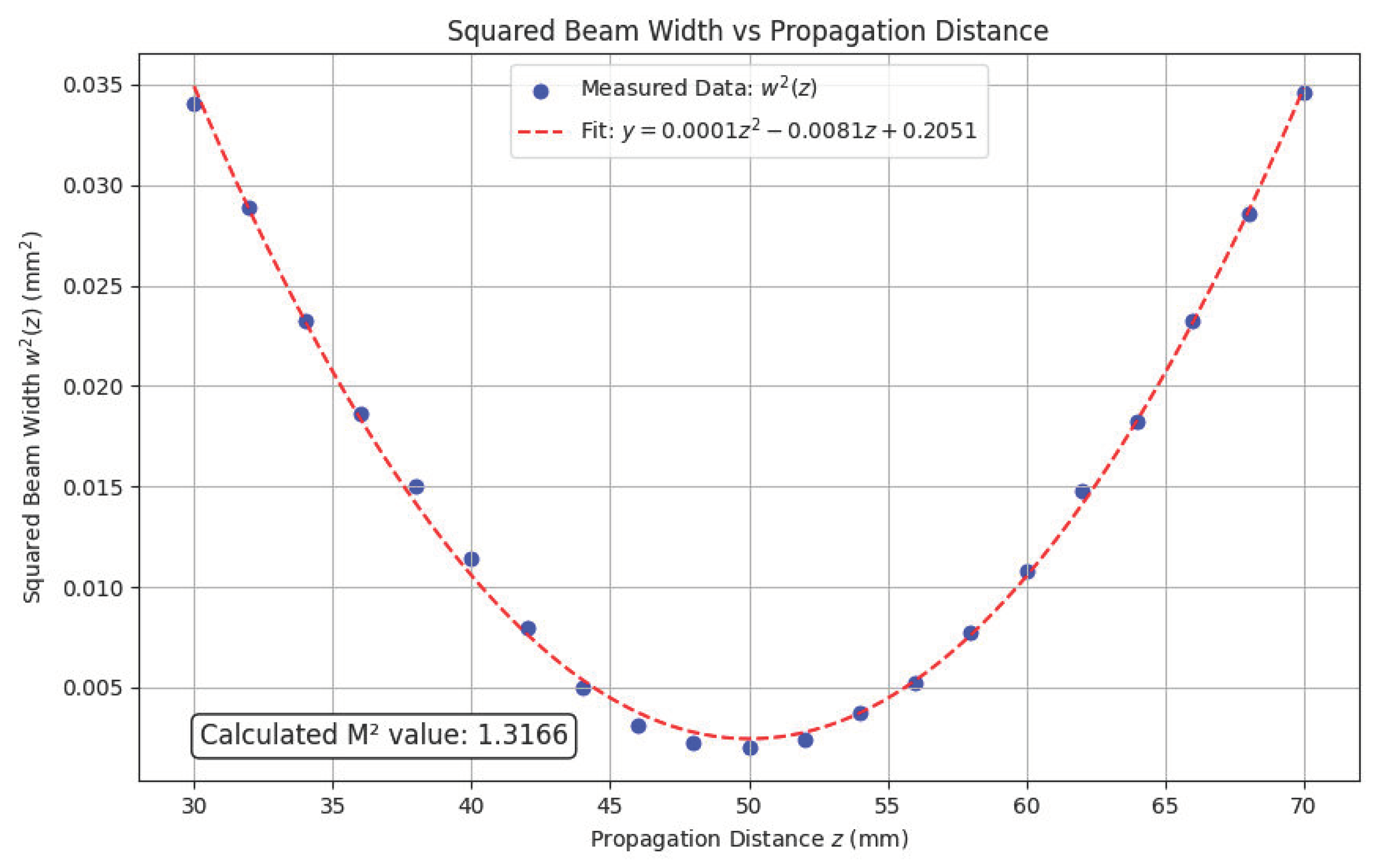
Figure 2.
Squared beam width vs. propagation distance with polynomial fit (DKE data).
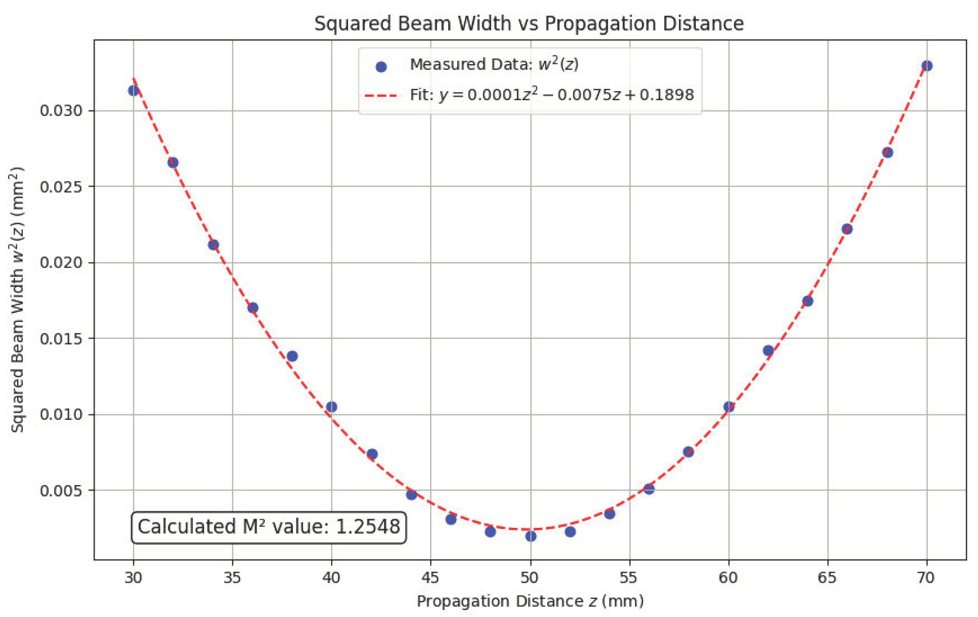

Table 1.
Beam Width Measurements using a Beam Gauge CCD Camera
| Z (mm) | D4 (mm) | DKE (mm) |
|---|---|---|
| 30 | 0.369 | 0.354 |
| 32 | 0.340 | 0.326 |
| 34 | 0.305 | 0.291 |
| 36 | 0.273 | 0.261 |
| 38 | 0.245 | 0.235 |
| 40 | 0.214 | 0.205 |
| 42 | 0.179 | 0.172 |
| 44 | 0.141 | 0.137 |
| 46 | 0.112 | 0.111 |
| 48 | 0.095 | 0.095 |
| 50 | 0.090 | 0.089 |
| 52 | 0.098 | 0.096 |
| 54 | 0.122 | 0.118 |
| 56 | 0.145 | 0.143 |
| 58 | 0.176 | 0.174 |
| 60 | 0.208 | 0.205 |
| 62 | 0.243 | 0.238 |
| 64 | 0.270 | 0.264 |
| 66 | 0.305 | 0.298 |
| 68 | 0.338 | 0.330 |
| 70 | 0.372 | 0.363 |
Disclaimer/Publisher’s Note: The statements, opinions and data contained in all publications are solely those of the individual author(s) and contributor(s) and not of MDPI and/or the editor(s). MDPI and/or the editor(s) disclaim responsibility for any injury to people or property resulting from any ideas, methods, instructions or products referred to in the content. |
© 2024 by the authors. Licensee MDPI, Basel, Switzerland. This article is an open access article distributed under the terms and conditions of the Creative Commons Attribution (CC BY) license (http://creativecommons.org/licenses/by/4.0/).
Copyright: This open access article is published under a Creative Commons CC BY 4.0 license, which permit the free download, distribution, and reuse, provided that the author and preprint are cited in any reuse.


