Submitted:
04 September 2024
Posted:
05 September 2024
You are already at the latest version
Abstract
Keywords:
1. Introduction
- A novel system architecture for random projection ensemble method that utilises the spare resources of an FPGA-based switch.
- A novel system architecture that enables kNN classification within FPGA-based network switches through an ensemble of classifiers with Hamming distance as the metric. The system can be easily adapted to FPGA-based NICs due to their similar architecture.
- Potential speedups in training whilst maintaining or even surpassing the single model accuracy for MLP-based classifiers.
- Achieving high memory reduction on high-dimensional dataset whilst retaining accuracy for kNN-based classifiers.
- A parameterised system model for hardware-software co-analysis that allows prediction and analysis of the system performance, for datasets of different sizes or FPGAs with different resources.
2. Background
2.1. FPGAs in the Network
2.2. Random Projection and Ensemble Classification
2.3. Previous Work on FPGA-Based kNN Design
2.4. Distance Metrics
- In classification, k-nearest neighbours (kNN) classifiers make predictions based on the distances between the input data point and its neighbours in the feature space.
- In kernel methods, certain kernel functions are related to specific distance metrics. For instance, the linear kernel is related to the dot product between vectors. The RBF Kernel (Gaussian Kernel) uses the Gaussian function, and its value is related to the Euclidean distance between data points.
- In recommendation systems, collaborative filtering often relies on distance metrics to measure the similarity between users or items. Similar users or items are recommended based on their historical preferences.
- In text mining and information retrieval, distance metrics, especially cosine similarity, are commonly used to compare and measure the similarity between documents or text snippets.
- In pattern recognition, distance metrics are utilised to quantify the similarity or dissimilarity between different patterns, whether they are in the form of images, sounds, or other types of data.
- Euclidean Distance: , which is often used in geometric contexts and when the dimensions are comparable.
- Manhattan Distance (L1 Norm): , which represents the distance between two points as the sum of the absolute differences along each dimension.
- Minkowski Distance: , which is a generalisation of both Euclidean and Manhattan distances. When , it reduces to the Euclidean distance; when , it becomes the Manhattan distance.
- Cosine Similarity: cosine_similarity, which measures the cosine of the angle between two vectors and is commonly used for text similarity and document clustering.
- Hamming Distance: , which is often used to compare strings of equal length, counting the number of positions at which the corresponding symbols differ.
2.5. Previous kNN Designs That Use Hamming Distance as the Metric
2.6. LSH Hashing
3. Proposed System Architecture
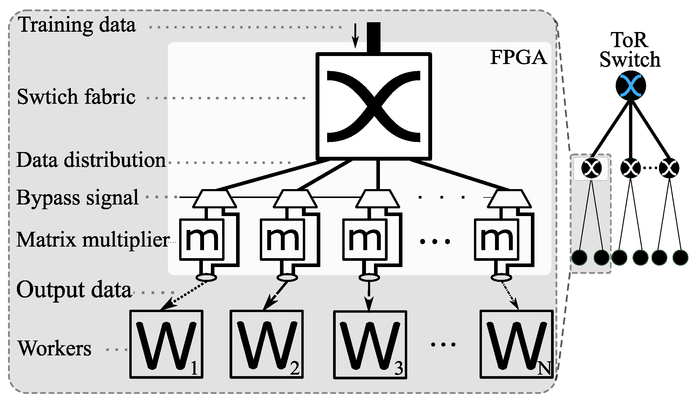
3.1. Overall System Design - for MLP-Based Models
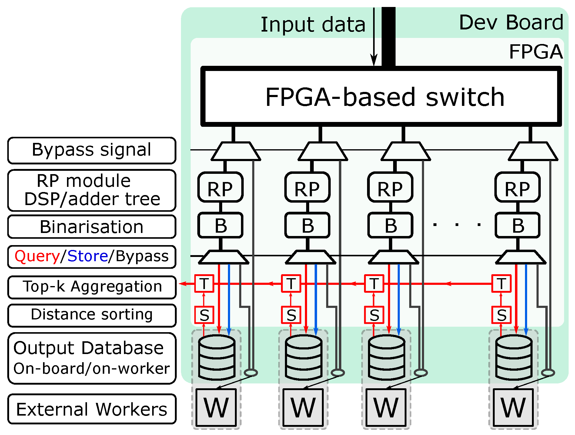
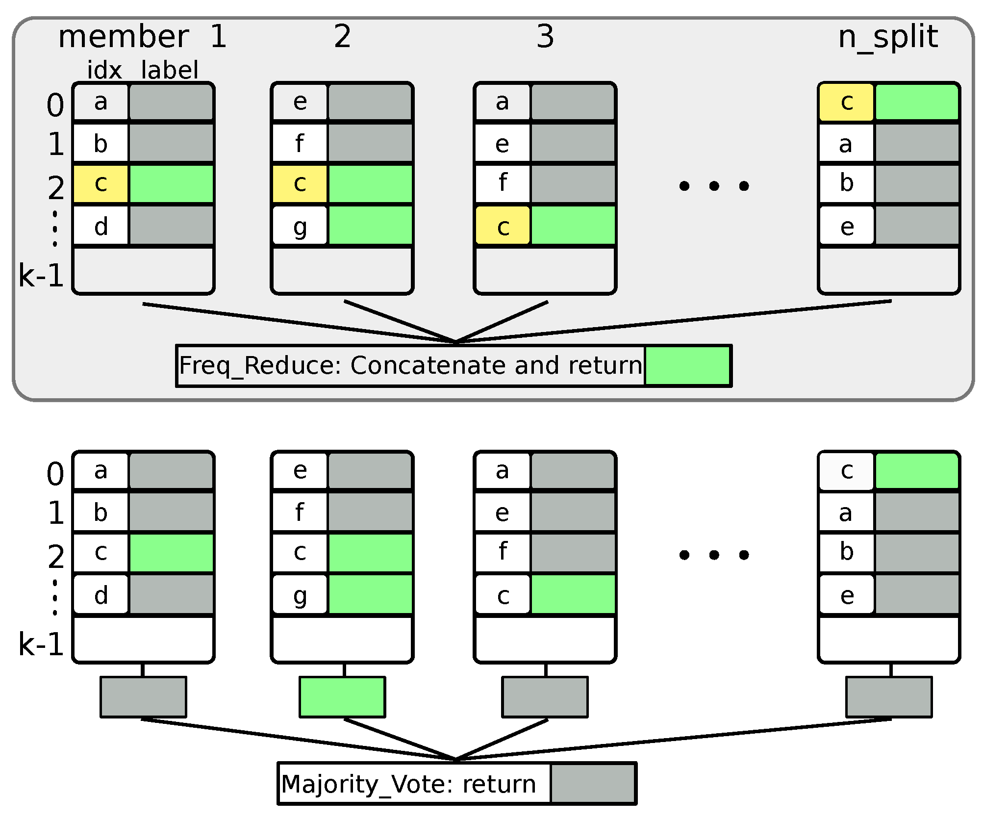
3.2. System Architecture for kNN Classifier with Hamming Distance as Metric
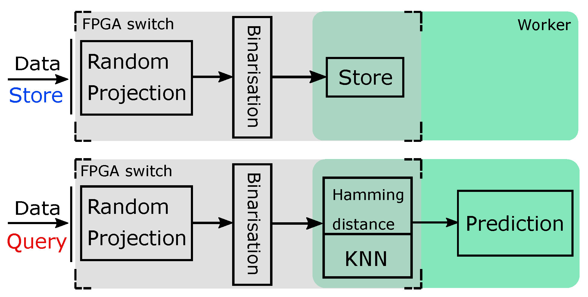
- An additional binarisation step to convert data to Hamming code and an additional level of multiplexing that supports the forward, store and query operations.
- In-FPGA top-k computation and aggregation on the Hamming code, which greatly reduces the computation overhead and, as a result, increases the performance. Converting to Hamming code also gives the FPGA the ability to store all data on-board. Therefore, the need to access data from the worker is eliminated (address challenge C3, C4).
- The multiplier module is not restricted to a DSP-based design, which enables support for different types of RP matrix.
4. Theoretical Model for MLP-Based Classifiers
- and . Since is the fundamental setting of random projection and , we have . Therefore inequality 7 obviously holds.
- and . In this case, . Therefore, similar to the previous case, inequality 7 still holds.
- and . In other words, the random projection time is the bottleneck of both systems. In this case, the inequity holds if , which holds as long as DSPs on the FPGA have a speed advantage over the server in terms of matrix multiplication.
- and . In this case, whether inequality 7 holds is more data-dependent and hardware-dependent. However, we found that the case is very unlikely to appear practically.
5. Experiment Setup and Performance Analysis for MLP-Based Classifier
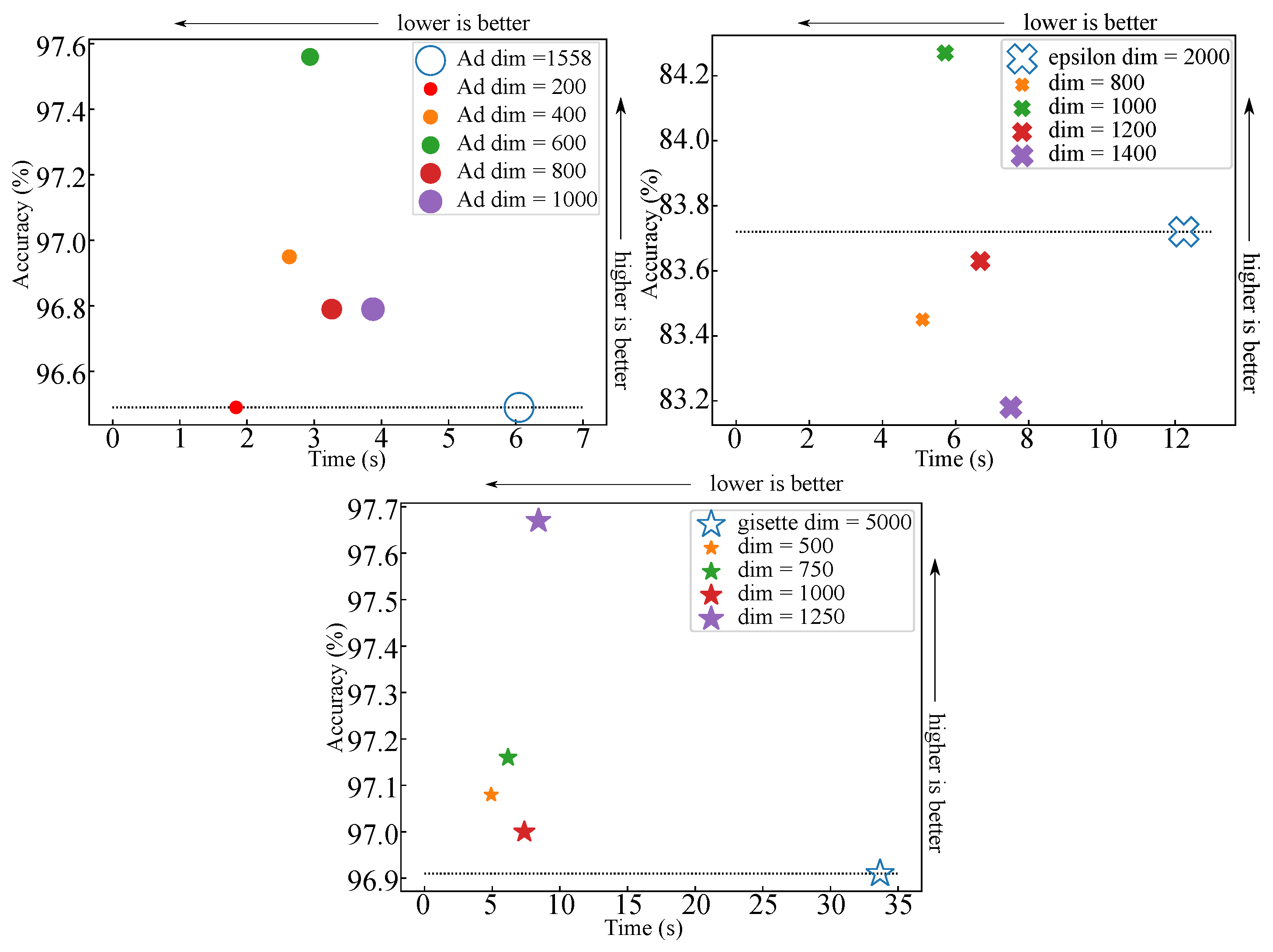
6. Dataset-Specific Case Study for MLP-Based Classifier
6.1. Time Estimation for Very Large Dimension Size
7. Experiment Setup and Performance Analysis for kNN-Based Classifier
7.1. Software Modelling
7.2. Performance Modelling
7.3. Dataset-Specific Case Study
| Name | # entry |
M | m | sp | Lib Time CPU Cosine/s |
Estimated time/s FPGA |
FPGA speedup |
Total memory reduction |
Trigger size Terabytes |
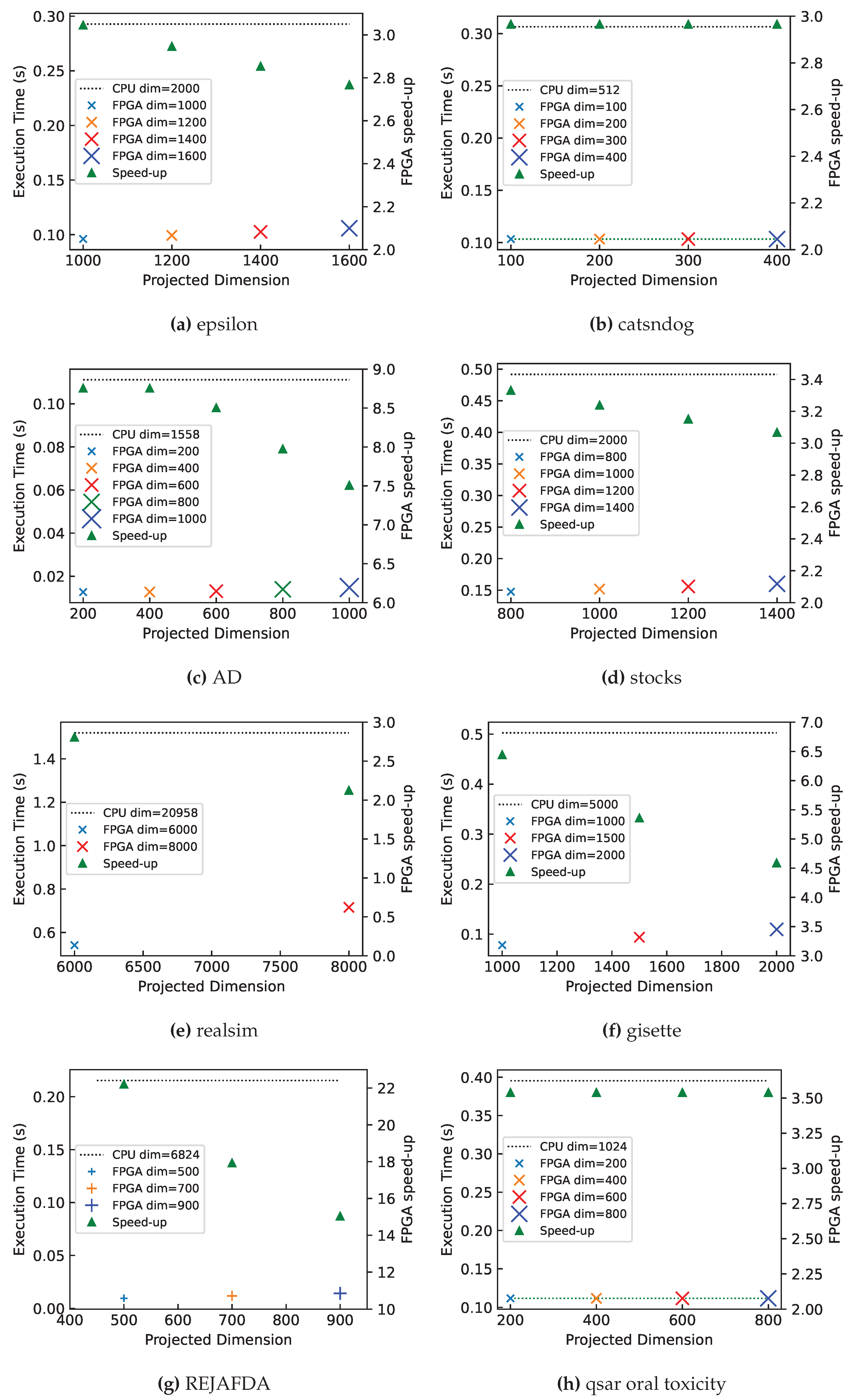
| epsilon [32] | 7000 | 2000 | 1000 | 0.9 | 0.2927 | 0.095917 | 3.05 | 3.95 | 1.138 |
| catsndogs | 10000 | 512 | 100 | 0.6 | 0.3065 | 0.103337 | 2.97 | 21.01 | 4.369 |
| AD [33] | 3279 | 1558 | 200 | 0.6 | 0.1111 | 0.012718 | 8.74 | 27.70 | 6.647 |
| stock | 10074 | 2000 | 1000 | 0.8 | 0.4916 | 0.151872 | 3.24 | 26.67 | 1.280 |
| realsim [34] | 3614 | 20958 | 8000 | 0.8 | 1.5200 | 0.652816 | 2.33 | 6.99 | 1.677 |
| gisette [35] | 6000 | 5000 | 1000 | 0.8 | 0.5027 | 0.078037 | 6.44 | 22.22 | 3.200 |
| REJAFDA [36] | 1996 | 6824 | 700 | 0.6 | 0.2153 | 0.012023 | 17.91 | 519.92 | 8.318 |
| qsar_oral [37] | 8992 | 1024 | 800 | 0.8 | 0.3953 | 0.111949 | 3.53 | 12.8 | 0.819 |
7.3.1. Quantifying the Gap between Forwarding Latency and Computation Latency
8. Discussion
8.1. MLP-Based Classifier
8.2. kNN-Based Classifier
8.2.1. Relationship between Speed-up and Projected Dimension
8.2.2. The Effect of Memory Reduction on System Scalability
| Designs | Platform | Metrics | Input Data dimension |
| [45] | AP | Euclidean | unspecified |
| [28] | AP | Hamming | 64 - 256 |
| CHIP-kNN [24] | Cloud FPGA | Euclidean | 2 - 128 |
| PRINS [46] | In-storage | Euclidean | 1 - 384 |
| kNN-MSDF [47] | FPGA SoC | Euclidean | 4 - 17 |
| [48] | FPGA SoC | Hamming | 64 |
| [29] | FPGA | Manhattan | 16384 |
| Rosetta [49] | FPGA | Hamming | unspecified |
| [50] | FPGA | Hamming | <24 |
| kNN-STUFF [51] | FPGA | Euclidean | <50 |
| [25] | FPGA | Euclidean | 64 |
| [52] | FPGA | Euclidean | 1 - 16 |
| [26] | FPGA | Euclidean | 16 |
| [53] | FPGA | Hamming | <50 |
| This work | FPGA network switch |
Hamming | <20958 |
9. Conclusion and Future Works
Acknowledgments
Conflicts of Interest
References
- Cooke, R.A.; Fahmy, S.A. A model for distributed in-network and near-edge computing with heterogeneous hardware. Future Generation Computer Systems 2020, 105, 395–409. [Google Scholar] [CrossRef]
- Amazon. Amazon EC2 F1 Instances.
- Firestone.; et al. Azure Accelerated Networking:{SmartNICs} in the Public Cloud. In Proceedings of the NSDI, 2018.
- N.McKeown. PISA: Protocol independent switch architecture. https://opennetworking.org/wp-content/uploads/2020/12/p4-ws-2017-p4-architectures.pdf, 2015.
- Hemmatpour, M.; Zheng, C.; Zilberman, N. E-commerce bot traffic: In-network impact, detection, and mitigation. In Proceedings of the 2024 27th Conference on Innovation in Clouds, Internet and Networks (ICIN). IEEE, 2024, pp. 179–185.
- Datta, S.; Kotha, A.; Venkanna, U.; et al. XNetIoT: An Extreme Quantized Neural Network Architecture For IoT Environment Using P4. IEEE Transactions on Network and Service Management 2024. [CrossRef]
- Zheng, C.; Xiong, Z.; Bui, T.T.; Kaupmees, S.; Bensoussane, R.; Bernabeu, A.; Vargaftik, S.; Ben-Itzhak, Y.; Zilberman, N. IIsy: Hybrid In-Network Classification Using Programmable Switches. IEEE/ACM Transactions on Networking 2024. [CrossRef]
- Nguyen, H.N.; Nguyen, M.D.; Montes de Oca, E. A Framework for In-network Inference using P4. In Proceedings of the Proceedings of the 19th International Conference on Availability, Reliability and Security, 2024, pp. 1–6.
- Paolini, E.; De Marinis, L.; Scano, D.; Paolucci, F. In-Line Any-Depth Deep Neural Networks Using P4 Switches. IEEE Open Journal of the Communications Society 2024. [CrossRef]
- Zhang, K.; Samaan, N.; Karmouch, A. A Machine Learning-Based Toolbox for P4 Programmable Data-Planes. IEEE Transactions on Network and Service Management 2024. [CrossRef]
- Cooke, R.A.; Fahmy, S.A. Quantifying the latency benefits of near-edge and in-network FPGA acceleration. In Proceedings of the EdgeSys, 2020.
- Li.; et al. Accelerating distributed reinforcement learning with in-switch computing. In Proceedings of the ISCA. IEEE, 2019.
- Meng, J.; Gebara, N.; Ng, H.C.; Costa, P.; Luk, W. Investigating the Feasibility of FPGA-based Network Switches. In Proceedings of the 2019 IEEE 30th International Conference on Application-specific Systems, Architectures and Processors (ASAP). IEEE, 2019, Vol. 2160, pp. 218–226.
- NetFPGA. NetFPGA SUME: Reference Learning Switch Lite. https://github.com/NetFPGA/NetFPGA-SUME-public/wiki/NetFPGA-SUME-Reference-Learning-Switch-Lite, 2021.
- Dai, Z.; Zhu, J. Saturating the transceiver bandwidth: Switch fabric design on FPGAs. In Proceedings of the FPGA, 2012, pp. 67–76.
- Papaphilippou, P.; et al. Hipernetch: High-Performance FPGA Network Switch. TRETS 2021. [CrossRef]
- Rebai, A.; Ojewale, M.A.; Ullah, A.; Canini, M.; Fahmy, S.A. SqueezeNIC: Low-Latency In-NIC Compression for Distributed Deep Learning. In Proceedings of the Proceedings of the 2024 SIGCOMM Workshop on Networks for AI Computing, 2024, pp. 61–68.
- Le, Y.; Chang, H.; Mukherjee, S.; Wang, L.; Akella, A.; Swift, M.M.; Lakshman, T. UNO: Uniflying host and smart NIC offload for flexible packet processing. In Proceedings of the Proceedings of the 2017 Symposium on Cloud Computing, 2017, pp. 506–519.
- Tork, M.; Maudlej, L.; Silberstein, M. Lynx: A smartnic-driven accelerator-centric architecture for network servers. In Proceedings of the Proceedings of the Twenty-Fifth International Conference on Architectural Support for Programming Languages and Operating Systems, 2020, pp. 117–131.
- Papaphilippou.; et al. High-performance FPGA network switch architecture. In Proceedings of the FPGA, 2020.
- Achlioptas, D. Database-friendly random projections: Johnson-Lindenstrauss with binary coins. JCSS 2003. [CrossRef]
- Li, P.; Hastie, T.J.; Church, K.W. Very sparse random projections. In Proceedings of the SIGKDD, 2006.
- Fox, S.; Tridgell, S.; Jin, C.; Leong, P.H. Random projections for scaling machine learning on FPGAs. In Proceedings of the 2016 International Conference on Field-Programmable Technology (FPT). IEEE, 2016, pp. 85–92.
- Lu.; et al. CHIP-KNN: A configurable and high-performance k-nearest neighbors accelerator on cloud FPGAs. In Proceedings of the ICFPT. IEEE, 2020.
- Pu, Y.; et al. An efficient knn algorithm implemented on FPGA based heterogeneous computing system using opencl. In Proceedings of the FCCM. IEEE, 2015.
- Song, X.; Xie, T.; Fischer, S. A memory-access-efficient adaptive implementation of kNN on FPGA through HLS. In Proceedings of the ICCD. IEEE, 2019.
- An, F.; Mattausch, H.J.; Koide, T. An FPGA-implemented Associative-memory Based Online Learning Method. IJMLC 2011. [Google Scholar] [CrossRef]
- Lee.; et al. Similarity search on automata processors. In Proceedings of the IPDPS. IEEE, 2017.
- Stamoulias, I.; et al. Parallel architectures for the kNN classifier–design of soft IP cores and FPGA implementations. TECS 2013. [Google Scholar] [CrossRef]
- Charikar, M.S. Similarity estimation techniques from rounding algorithms. In Proceedings of the STOC, 2002.
- Indyk, P.; Motwani, R. Approximate nearest neighbors: towards removing the curse of dimensionality. In Proceedings of the STOC, 1998.
- LIBSVM Data: Classification (Binary Class). https://www.csie.ntu.edu.tw/~cjlin/libsvmtools/datasets/binary.html#epsilon.
- Kushmerick, N. Internet Advertisements. UCI Machine Learning Repository, 1998. [CrossRef]
- LIBSVM Data: Classification (Binary Class). https://www.csie.ntu.edu.tw/~cjlin/libsvmtools/datasets/binary.html#real-sim.
- Guyon, I.; Gunn, S.; Ben-Hur, A.; Dror, G. Gisette. UCI Machine Learning Repository, 2008. [CrossRef]
- Pinheiro, R.; et al. REJAFADA. UCI Machine Learning Repository, 2023. [CrossRef]
- QSAR oral toxicity. UCI Machine Learning Repository, 2019. [CrossRef]
- Dua, D.; Graff, C. UCI Machine Learning Repository, 2017.
- Chollet, F.; et al. Keras. https://keras.io, 2015.
- Zilberman, N.; et al. NetFPGA SUME: Toward 100 Gbps as research commodity. IEEE micro 2014. [Google Scholar] [CrossRef]
- Kushmerick, N. Learning to Remove Internet Advertisements. In Proceedings of the Agents, 1999, p. 175.
- Xilinx. Alveo U280 Data Center Accelerator Card.
- Radford.; et al. Learning transferable visual models from natural language supervision. In Proceedings of the ICML. PMLR, 2021.
- Meng.; et al. Fast and accurate training of ensemble models with FPGA-based switch. In Proceedings of the ASAP. IEEE, 2020.
- Lee.; et al. Application codesign of near-data processing for similarity search. In Proceedings of the IPDPS. IEEE, 2018.
- Kaplan, R.; et al. PRINS: Processing-in-storage acceleration of machine learning. IEEE Transactions on Nanotechnology 2018. [Google Scholar] [CrossRef]
- Gorgin.; et al. kNN-MSDF: A Hardware Accelerator for k-Nearest Neighbors Using Most Significant Digit First Computation. In Proceedings of the SOCC. IEEE, 2022.
- de Araújo.; et al. Hardware-Accelerated Similarity Search with Multi-Index Hashing. In Proceedings of the DASC/PiCom/CBDCom/CyberSciTech. IEEE, 2019.
- Zhou.; et al. Rosetta: A realistic high-level synthesis benchmark suite for software programmable FPGAs. In Proceedings of the FPGA, 2018.
- Ito.; et al. A Nearest Neighbor Search Engine Using Distance-Based Hashing. In Proceedings of the ICFPT. IEEE, 2018.
- Vieira, J.; Duarte, R.P.; Neto, H.C. kNN-STUFF: kNN STreaming unit for FPGAs. IEEE Access 2019. [Google Scholar] [CrossRef]
- Hussain, H.; et al. An adaptive FPGA implementation of multi-core K-nearest neighbour ensemble classifier using dynamic partial reconfiguration. In Proceedings of the FPL. IEEE, 2012.
- Jiang, W.; Gokhale, M. Real-time classification of multimedia traffic using FPGA. In Proceedings of the ICFPL. IEEE, 2010.
| 1 |

| Name | number of instances | original dimension |
| epsilon [32] | 7000 | 2000 |
| catsndogs | 10000 | 512 |
| AD [33] | 3279 | 1558 |
| stock | 10074 | 2000 |
| realsim [34] | 3614 | 20958 |
| gisette [35] | 6000 | 5000 |
| REJAFDA [36] | 1996 | 6824 |
| qsar_oral [37] | 8992 | 1024 |
| Name | Size used |
Original dimension |
Reduced dimension |
Estimated Speedup |
| Ad [41] | 3279 | 1558 | 200 | 3.28 |
| epsilon [32] | 55000 | 2000 | 1000 | 2.12 |
| gisette [38] | 6000 | 5000 | 1000 | 6.77 |
| realsim [34] | 5783 | 20958 | 3500 | 3.51 |
| Random projection time (s) | |||
| Name | |||
| Ad | 0.1145 | 0.0021 | 0.980 |
| epsilon | 0.1867 | 0.1760 | 0.515 |
| gisette | 0.3686 | 0.0320 | 0.920 |
| realsim | 0.7012 | 0.7756 | 0.475 |
| RP Matrix type | Multiplier | Sparsity | Data type/value |
| Gaussian | DSP | Dense | floating-point |
| GaussianInt | Adder tree | Dense | integer (0, 1, -1) |
| Sparse | DSP | Sparse | floating-point |
| SparseInt | Adder tree | Sparse | integer (0, 1, -1) |
| latency (cycles) |
Latency (absolute) |
Interval (cycles) |
Type |
| 81951 | 0.410ms | 6304 | dataflow |
| Resource | LUT | BRAM | FF | DSP |
| Total | 1303680 | 4032 | 2607360 | 9024 |
| Used | 7421 | 192 | 3755 | 0 |
| Used% | 0.57% | 4.76% | 0.14% | 0.00% |
Disclaimer/Publisher’s Note: The statements, opinions and data contained in all publications are solely those of the individual author(s) and contributor(s) and not of MDPI and/or the editor(s). MDPI and/or the editor(s) disclaim responsibility for any injury to people or property resulting from any ideas, methods, instructions or products referred to in the content. |
© 2024 by the authors. Licensee MDPI, Basel, Switzerland. This article is an open access article distributed under the terms and conditions of the Creative Commons Attribution (CC BY) license (http://creativecommons.org/licenses/by/4.0/).


