2. The 4th Order Runge-Kutta Solver for the Spin Bloch Equations
The spin Bloch equations can be solved in Matlab by constructing a fourth-order Runge-Kutta solver. Given the Bloch equations
I can specify field parameters, time steps, simulation time and initial conditions as inputs into my RK4. For spin dressing, I simply have to use the appropriate fields and solve for the spin components. The fields will be
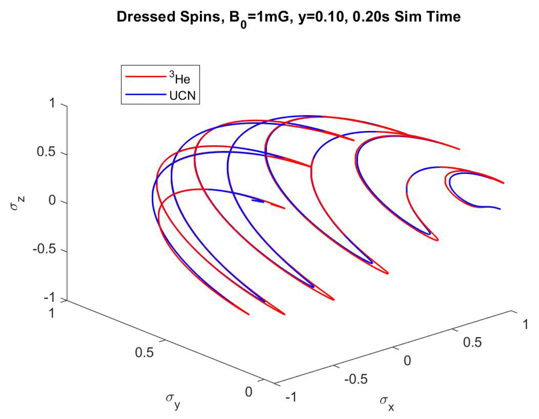
An example of a three dimensional spin dressing simulation between UCN and
3He is shown in
Figure 1.
Using initial conditions on the time dependent spin components of , and , time steps of seconds for the spin components and for magnetic field time steps, the RK4 will solve for each spin time series.
For the rest of this chapter, the simulation time is
(the actual computation can take anywhere from minutes to hours). For the number of particles, I will use
. Finally, the first results I will show have field parameters of
The results are spins as a function of time:
,
and
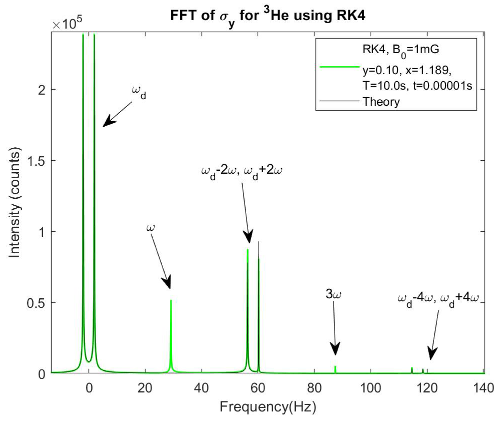
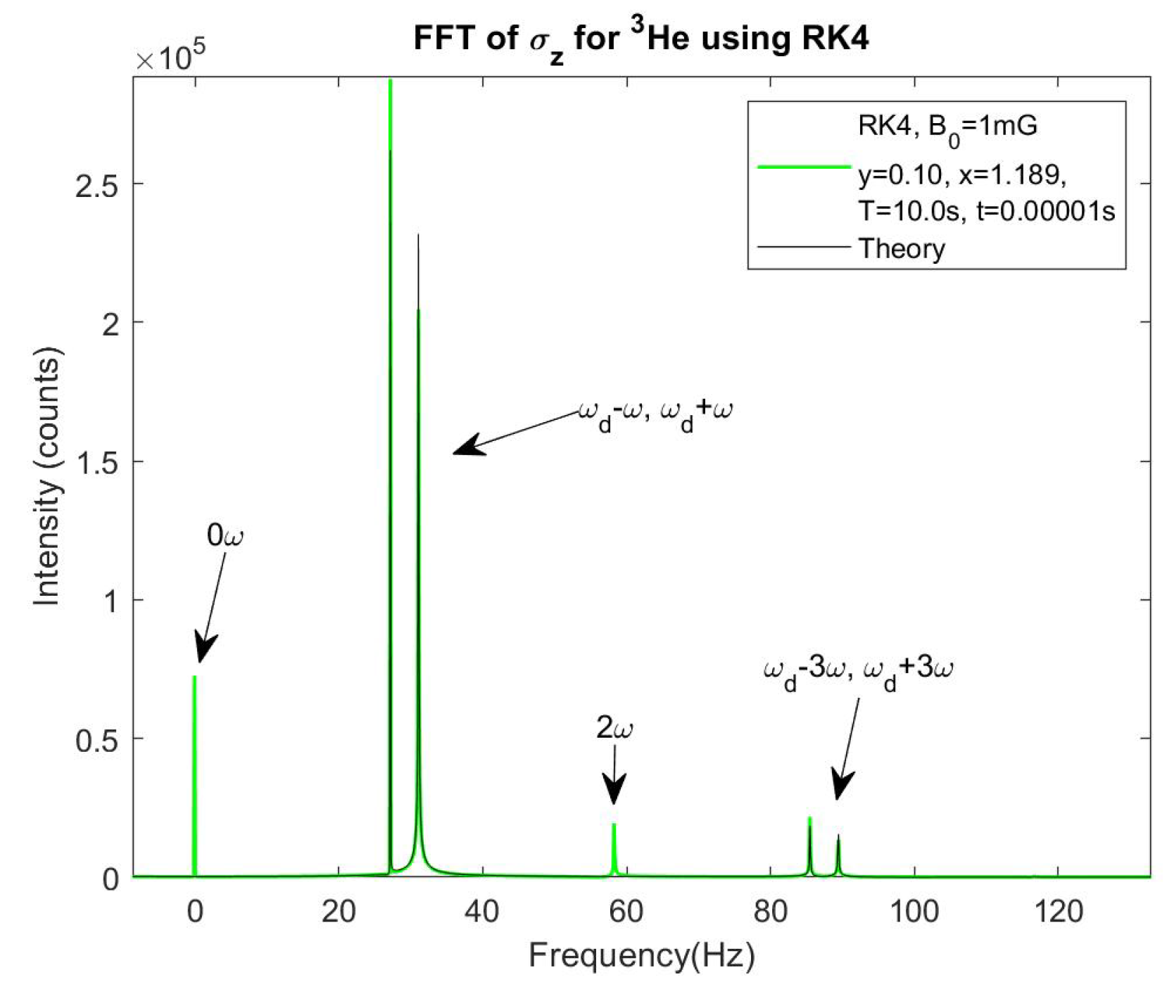
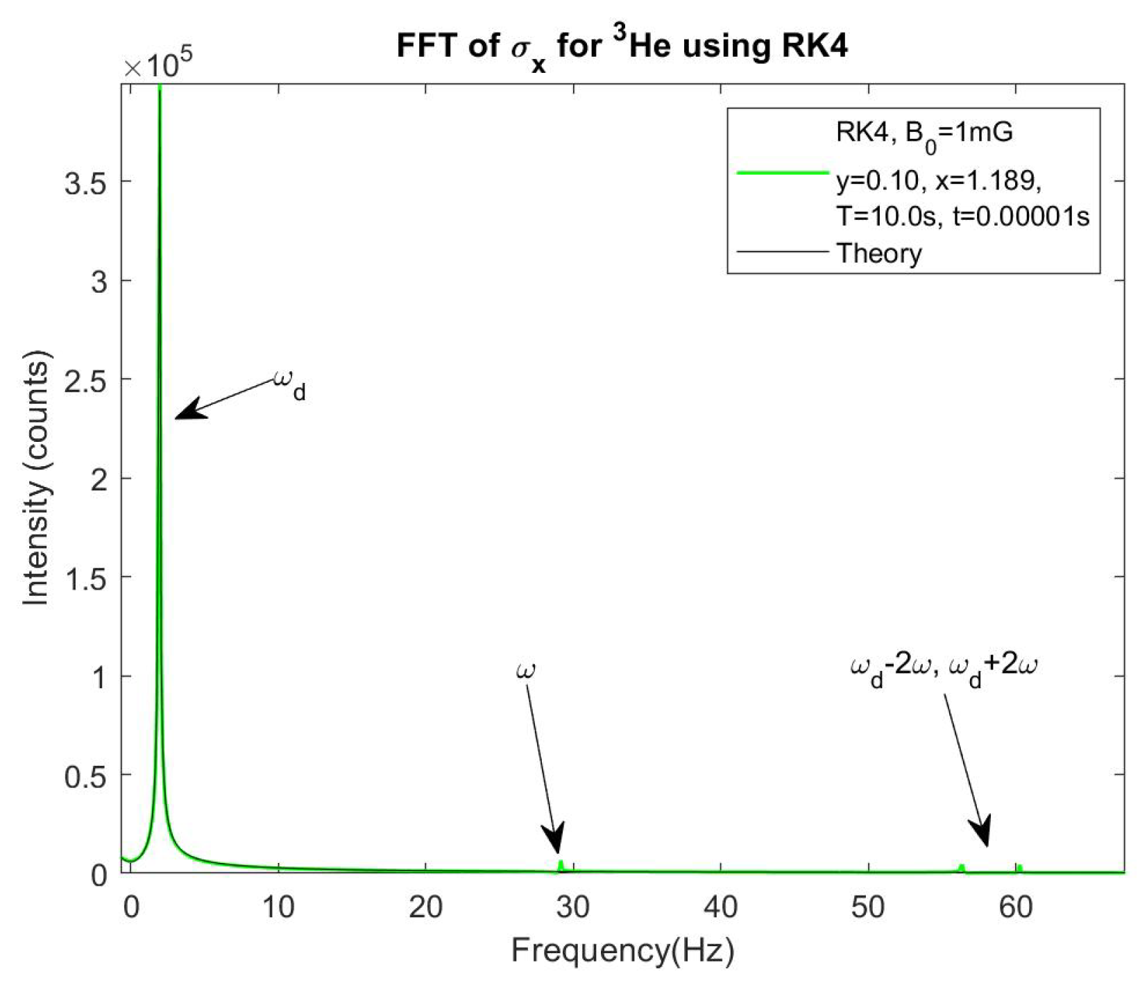
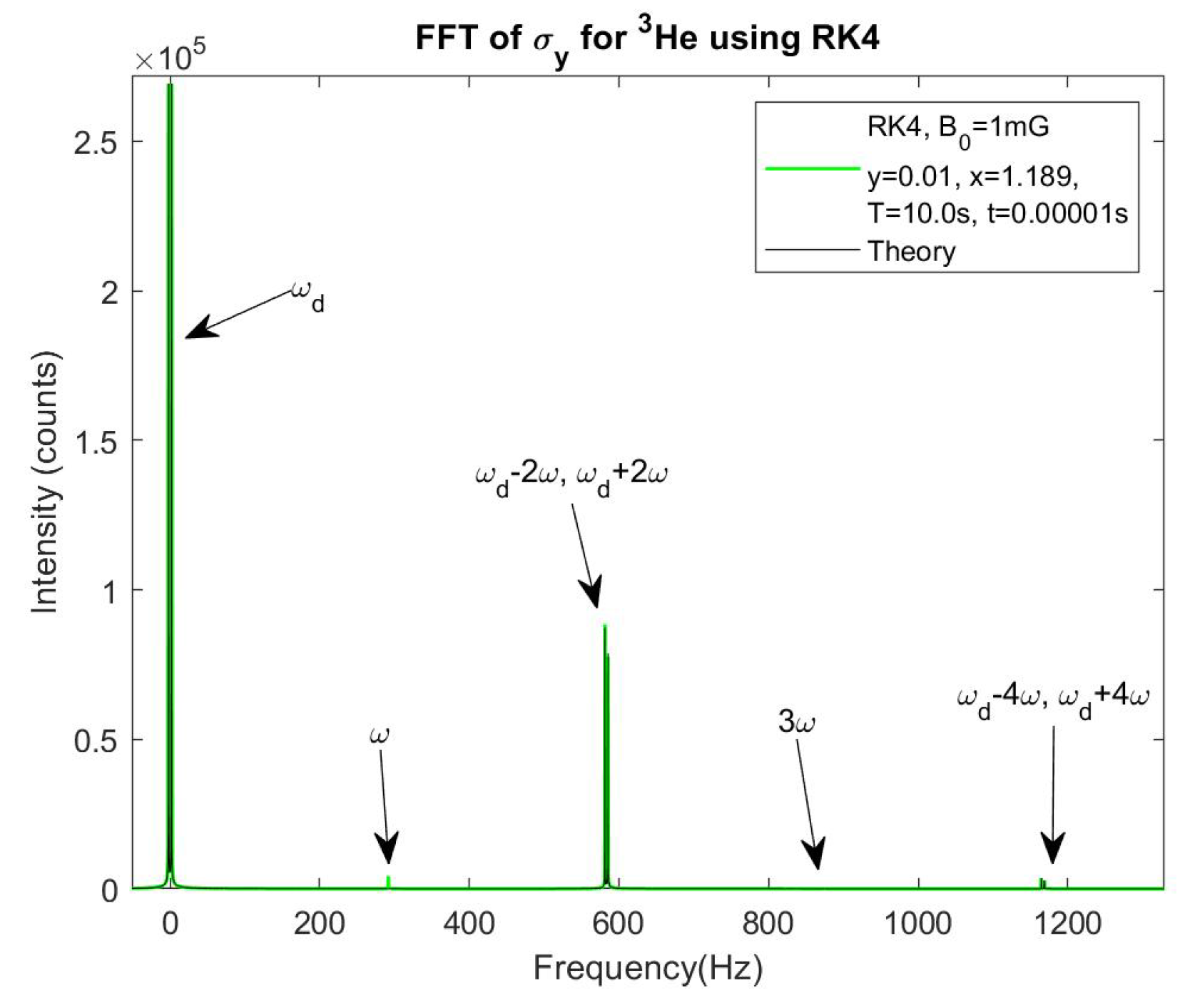
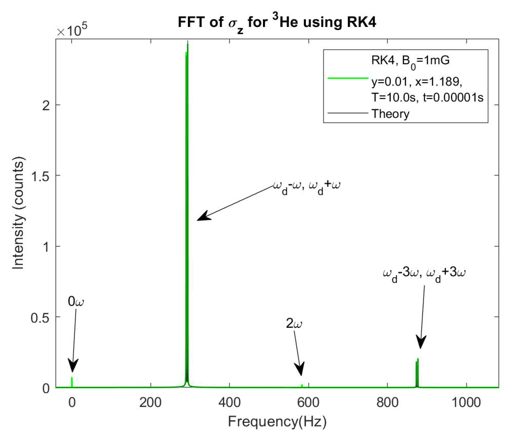
. I then take the fast Fourier transform (FFT) of these time series and to see relevant frequencies. From the theory in the previous section, I expect certain frequencies for each spin component. The plots in
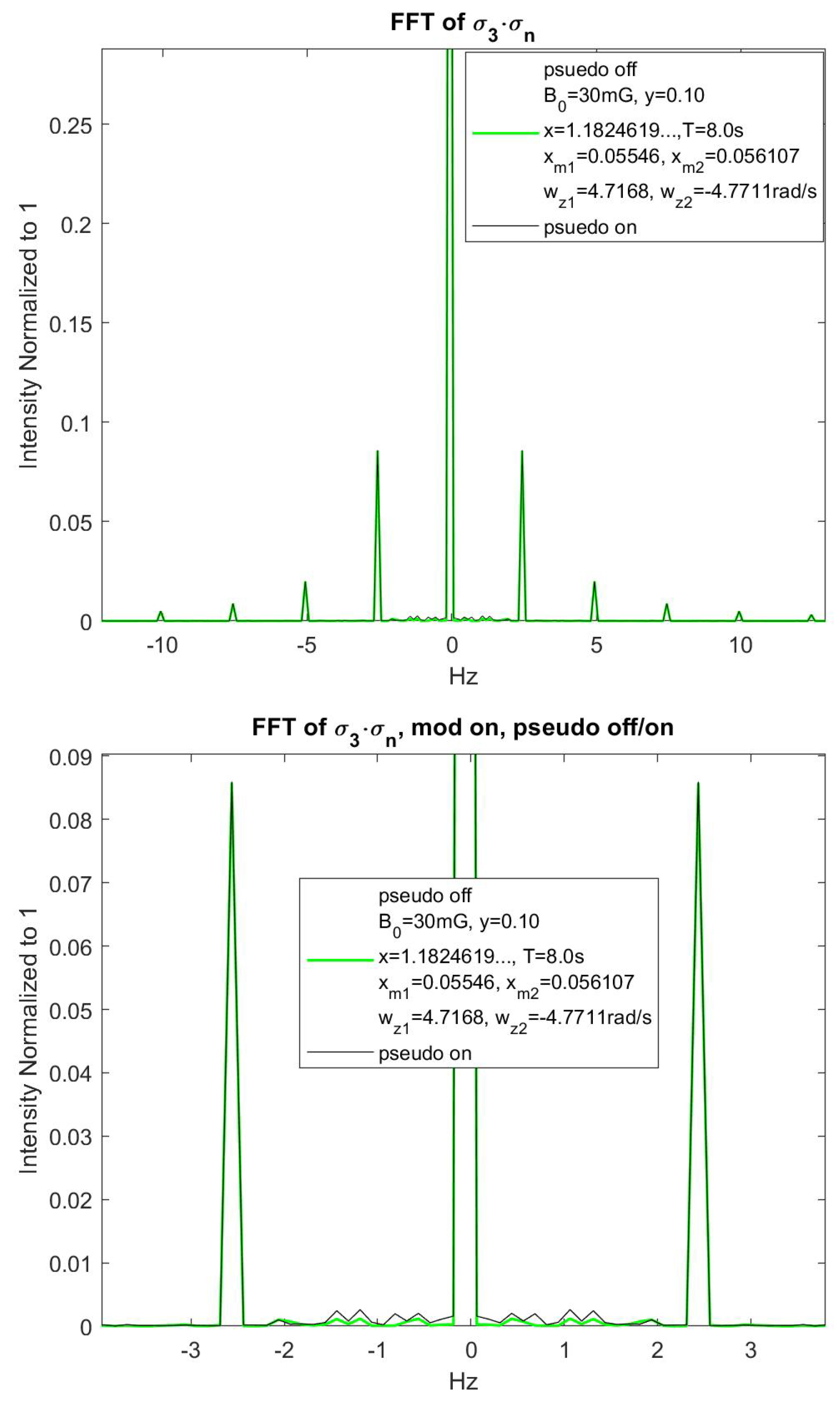
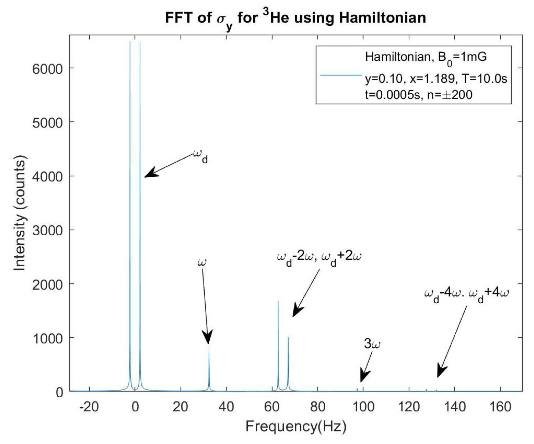
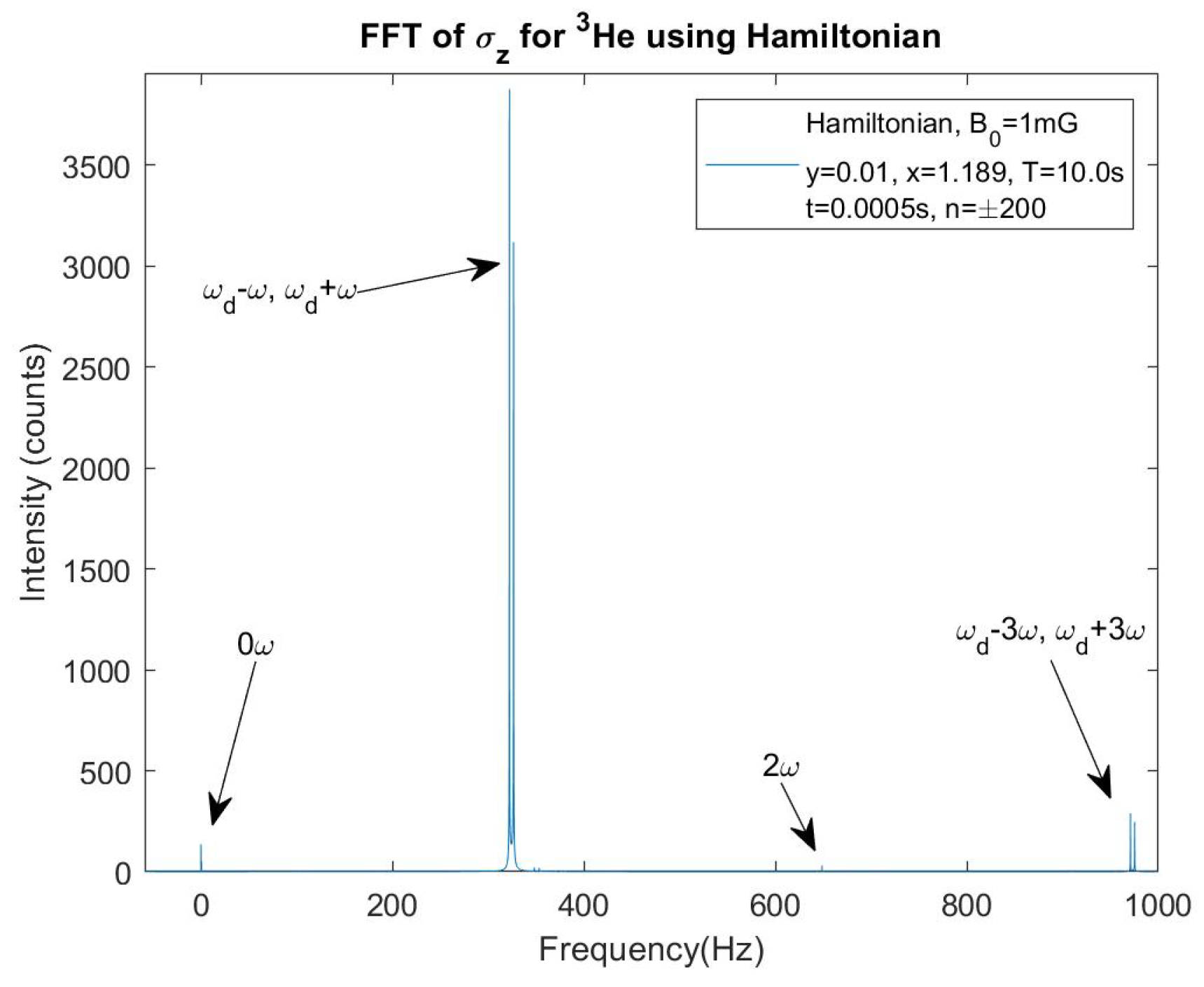
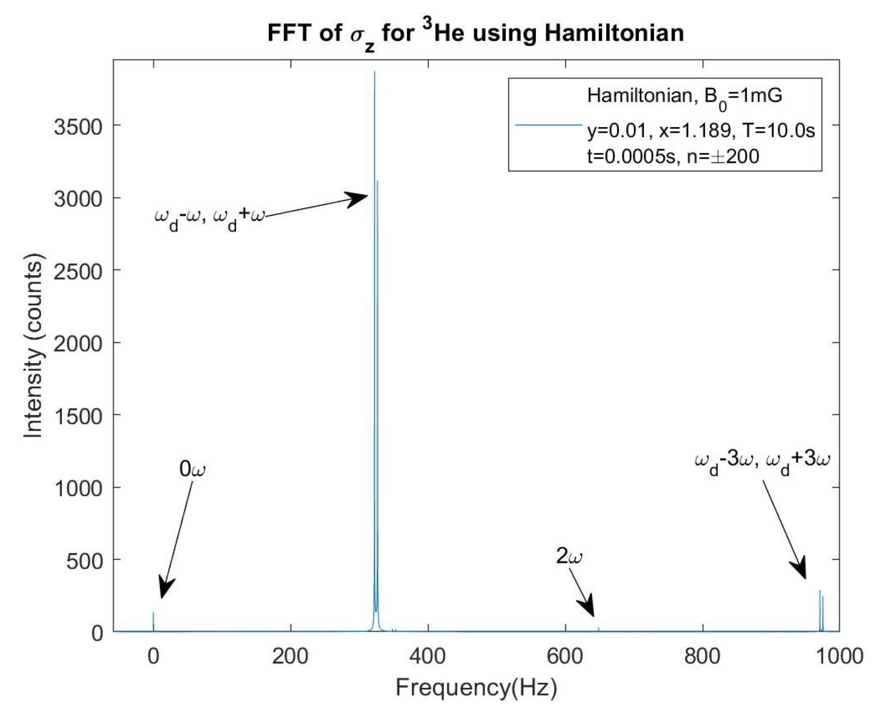
Figure 2 to 4 are the FFTs of the spins for the parameters in Equation 15. In light green is simulation data and in black is theory using the expectation values from last section. The time steps are very small and therefore the frequency range is large so the plots are zoomed in for better inspection of the relevant frequencies.
The theory in
Figure 2-4 are the predicted results from Equations 8, 10 and 12, respectively. As seen, there are frequencies and harmonics consistent with the expectation values in that section. Furthermore, the ratio of the heights of the expected peaks are in-line with ratios of amplitudes of Bessel functions of the first kind of corresponding order. But what is quite interesting are the peaks that the theory doesn’t predict. In
Figure 4 for
, I see these ’unexpected’ frequencies of
and
are almost negligible. But in
Figure 2 showing
, the unexpected peaks at
and
are not negligible. And for
in
Figure 3, the unexpected frequencies of
and
have meaningful intensities as well.
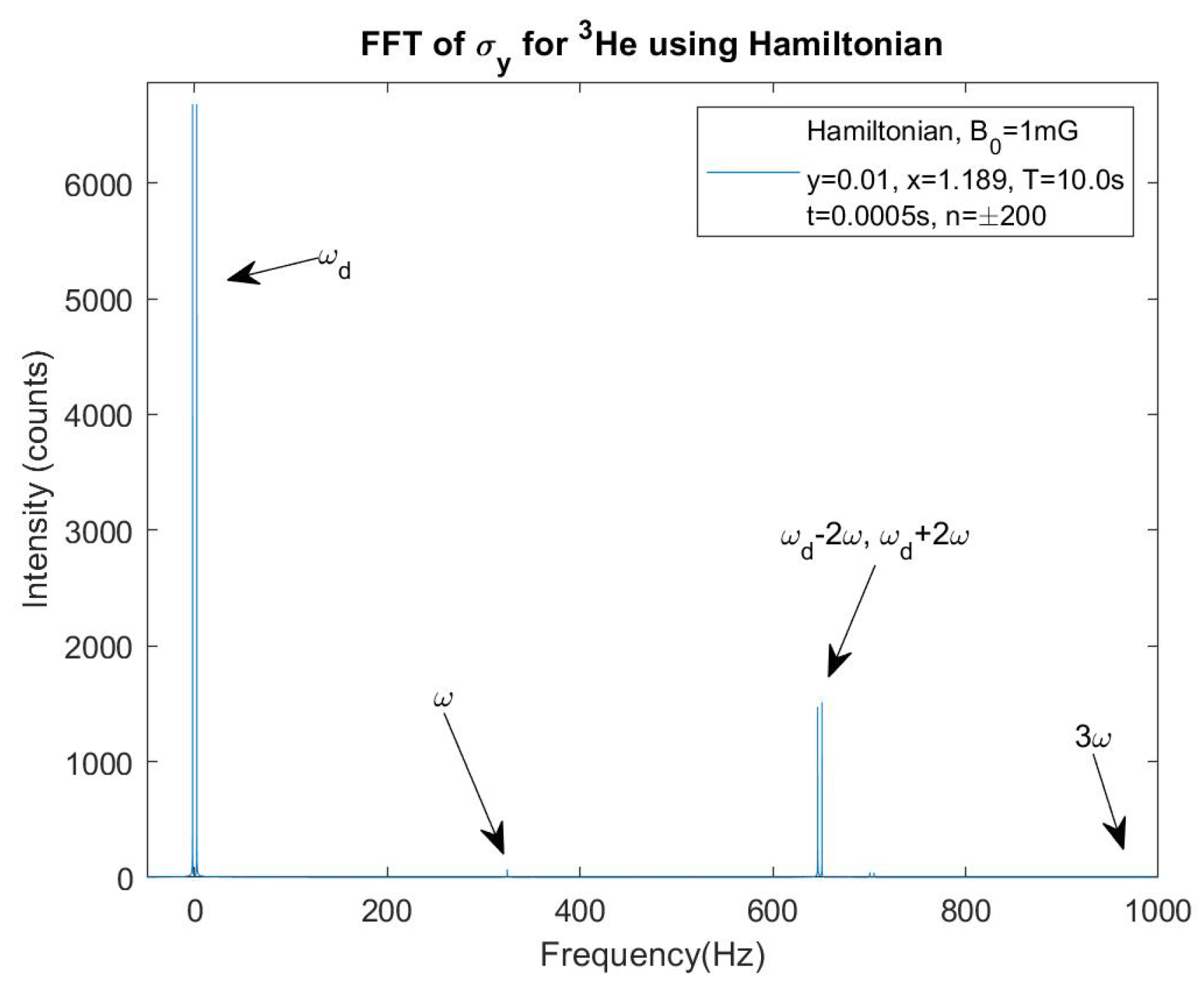
Figure 5 and 6 show what
Figure 3 and 4 showed but for
meaning
is ten times larger.
What’s interesting is that the unexpected frequencies decreased in height substantially between and . Given y is a measure of the perturbing static field relative to the rate of oscillation of the dressing field, intensity dependence on y points to missing higher order perturbation theory terms.
The question then is: are these unexpected frequencies due to the RK4 numerical solver issues in Matlab or is it from higher order perturbation theory terms? The reduction in intensity when
y is smaller would suggest the latter. Some theoretical models use
y anywhere between 0.10 and 0.01 while the experiment will use
.
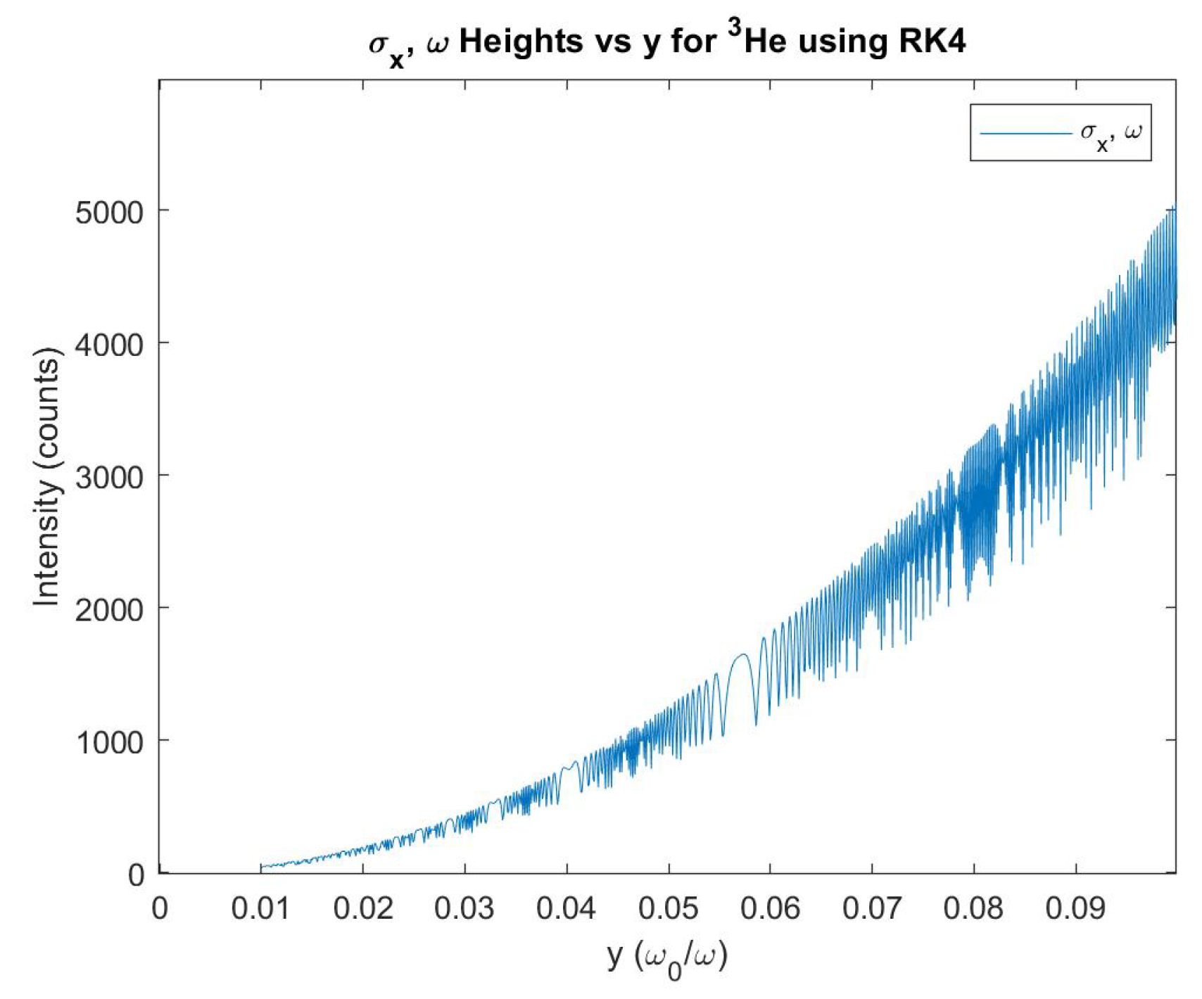
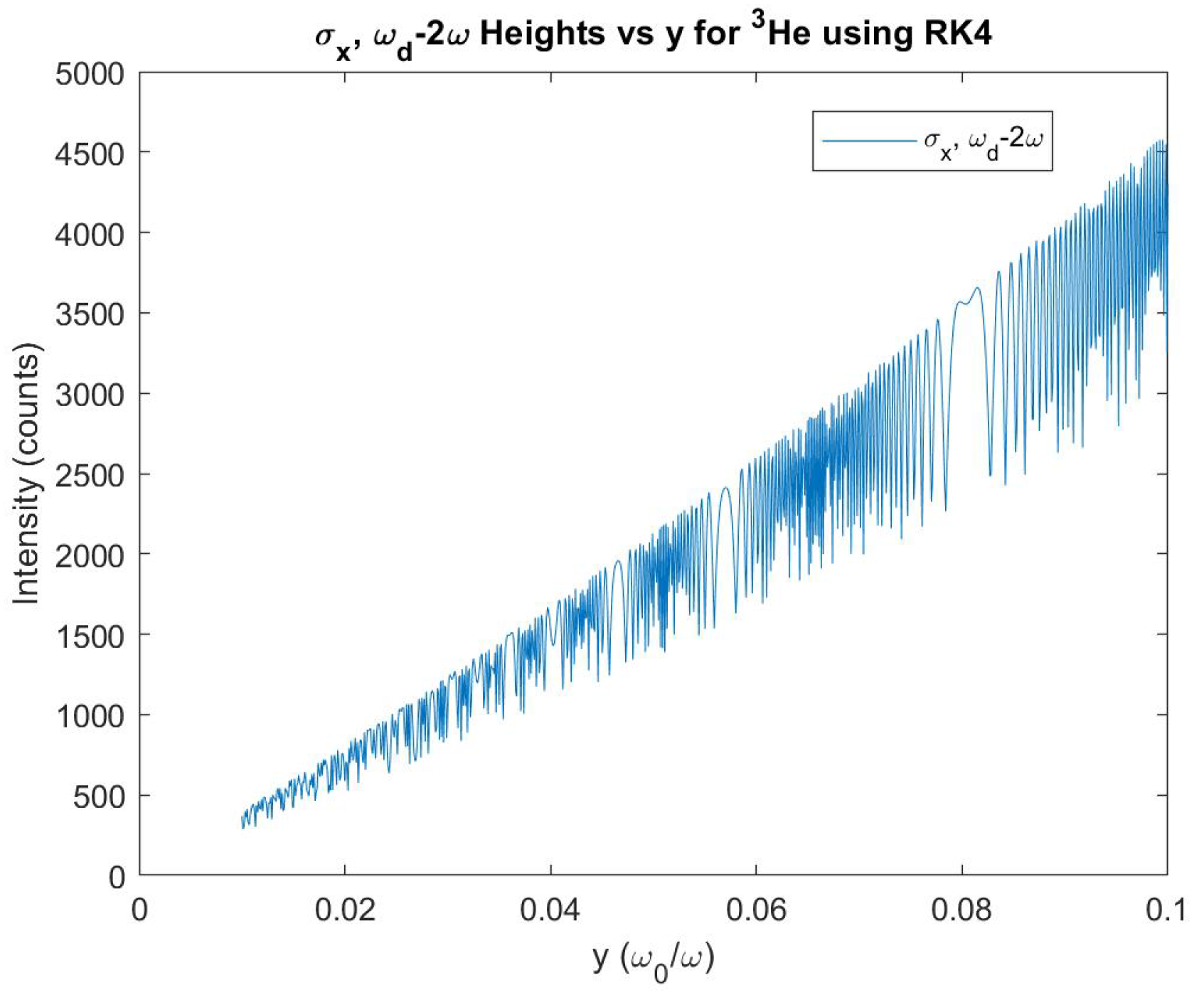
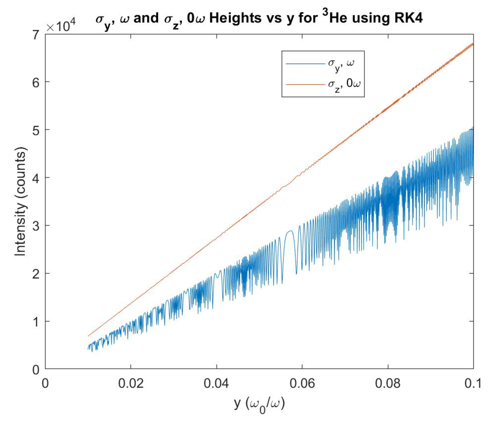
Figure 7 to 9 show how these unexpected frequency peaks change as the perturbation strength changes. I chose two frequencies from
(
and
) and one each from
(
) and
(
). Then stepped y by 0.0001 between 0.01 and 0.10.
The oscillatory behavior in
Figure 7 to 9 most likely comes from numerical issues within the solver. From
Figure 9, the unexpected frequencies I chose from
and
show linear in
y dependence. And from
Figure 7 and 8, unexpected frequencies for
show
and y dependence respectively. Going forward, I will call these unexpected frequencies
.
Given the dependence on y, the anomalies most likely come from perturbation theory. The next section shows a different method for solving for expectation values and frequencies of spin components to provide further evidence that the anomalies are not artifacts. If it can give confluence to the RK4 method, I will use higher order perturbation theory to more accurately represent this system.
4. First Order Perturbation Theory, Corrections to the Eigenstates
In the first section, the degeneracy was lifted by finding first order energy shifts. The eigenvectors were then used for calculating expectation values. Given the evidence laid out in the sections showing results from the RK4 and Hamiltonian methods, it’s clear extensions of perturbation theory are needed to account for the anomalous frequencies. More specifically, corrections to the eigenstates are required rather than corrections to the eigenvalues. This is because the only way for the peak heights to have a dependence on , where n is the order of perturbation theory, is from corrections to the eigenstates. Whereas corrections to the eigenvalues introduce changes to energy levels and therefore frequencies.
An expansion of an eigenstate using higher order corrections is written as

The first term on the right hand side are the
eigenstates whereas the second term is the 1st order correction.

The first order correction is generally written as

and so first order corrections to unprimed and primed states are
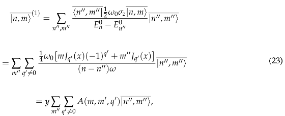
where I define
A as
For the primed states
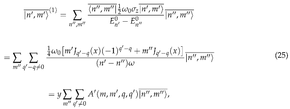
where I define
as
From before,
but now
such that
. States cannot be equal in the formulation of the first order corrections which then requires
and
for certain values of
but also to avoid singularities.
Now a state up to first order is

And similarly, a state
up to first order is
The matrix elements for are
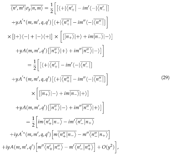
where the first two terms in the brackets are the usual zeroth order, unperturbed terms and
refers to terms proportional to
that I will ignore. Then, the expectation value is
Next I will choose
so that
no longer contributes to any frequency. Then, I examine the four cases when
and
. These calculations are located in the appendix in B. I know from the RK4 and diagonalizing the Hamiltonian that for
, the anomalous peaks are for odd
q. Choosing odd
q, then varying
(which dictates whether
is even or odd), I have
with
and
commuting. Of the four terms in Equation 31, the first and the fourth will be equal but opposite sign for certain
q and
values. Whereas the second and the third will be equal and same sign. I will show two examples of this when
and I choose different values of
based off the sum rules in Appendix C.
Finally, the expectation value for
and odd
q can be written as
The first few terms are
For all the other cases (
with
q odd or even and
with even
q) all terms vanish.
For , the matrix elements are
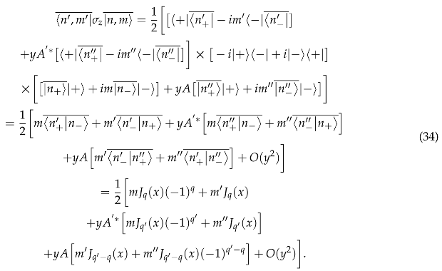
So that the expectation value up to y is
This time, I’ll exclude the zeroth order terms. The calculation for the sum over spins for
is similar to the
calculation. Then the linear in y terms are
For
, I saw the anomalies are for even
q. Then I have
with the first 4 terms being
Regarding
, I saw anomalous frequencies at
and
. The matrix elements for
are
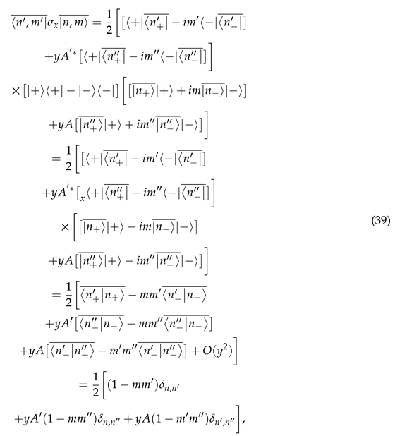
so that the expectation value is
For summing over all
n’s and
m’s in Equation 40, I have the following cases and their constraints (due to
in the formulation for first order perturbation theory)
Of these four cases, the first leads to the zeroth order
term. The second case has
and
which is not allowed. Cases three and four are the ones I care about. Given I’m in a spin 1/2 system, a constraint like
means
and so I can simply replace all
’s by
. Also, the third case has
so that any
can be replaced by
q. And the fourth case has
but given
, there’s no singularity. The calculation for the third case is
And the fourth case
Adding together the results from the third and fourth cases gives the full linear in y dependence of
as
From the results of Equation 44, it can be seen that the
for even
q, anomaly has be resolved. Also just as important is that the
anomaly did not show itself since data in the earlier section suggested it would depend on
. The
terms from the first order corrections that I ignored plus the
terms that would come about in second order corrections should show the frequencies
for odd
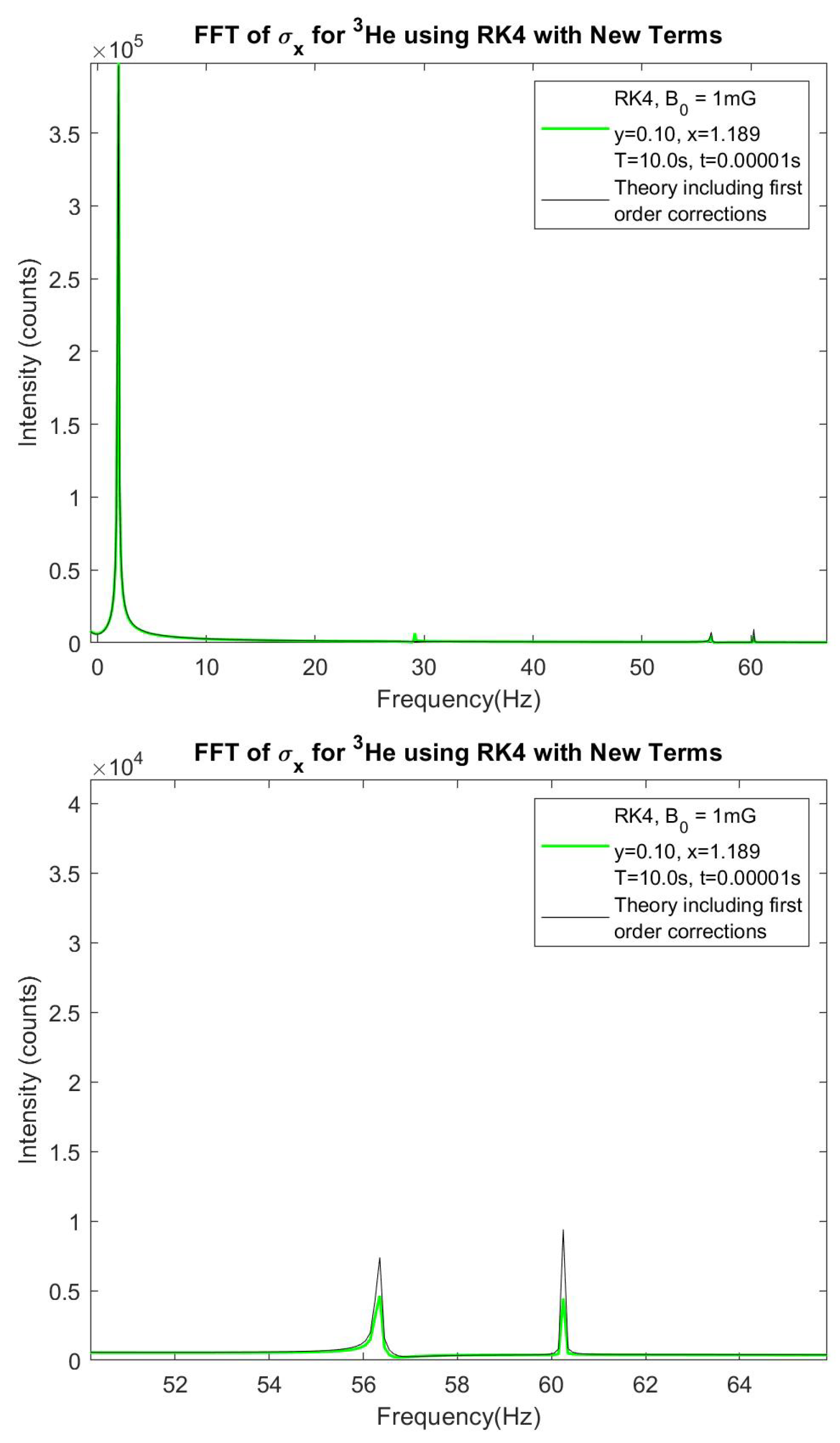
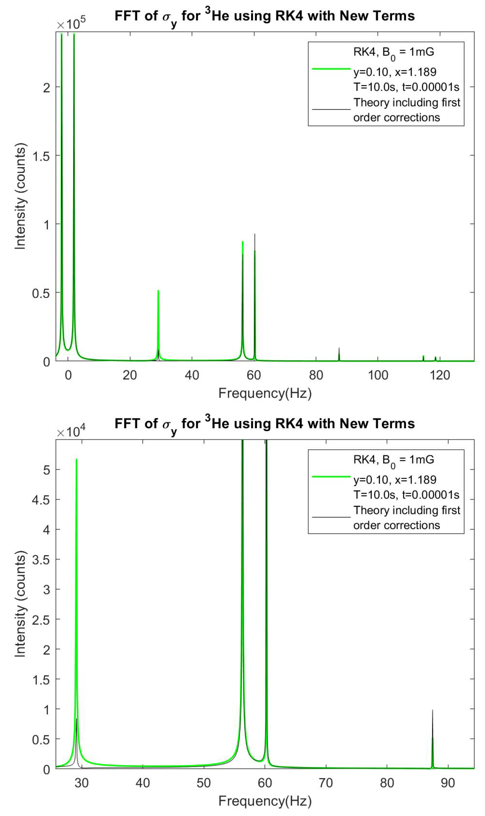
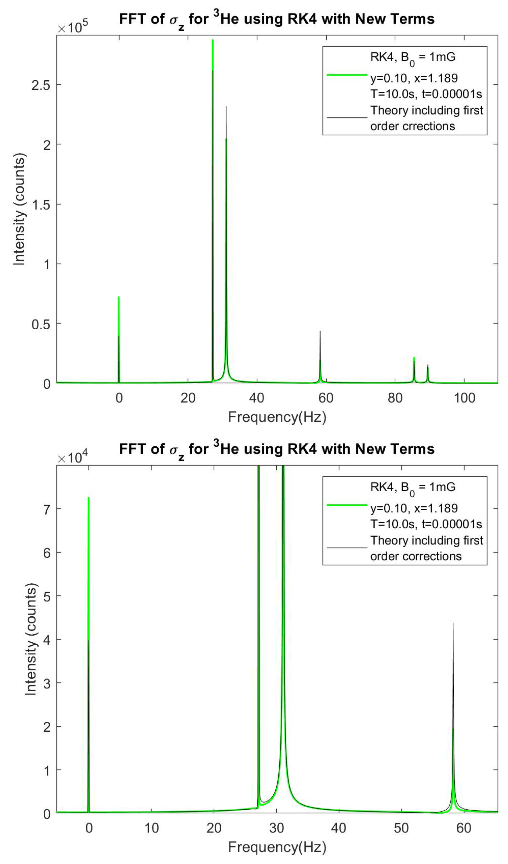
q. The plots with the first order corrections added to the theory, analogous to
Figure 2 to 4 are shown below in
Figure 15 to 17.
In
Figure 15, the
theoretical heights in black from the first order corrections are too large. In
Figure 16, the
theory peak is too small while the
is too large.
Figure 17 has discrepancies between RK4 heights and the new terms added to the theory as well. I also simply used 0.10 as a placeholder for the
oscillatory term. The differences are most likely due to either factors of 2 missing for certain frequency amplitudes, missing Bessel function terms since I stopped the sums after two terms or issues with normalization for Fourier transforms in Matlab.
What has been demonstrated is that the approximation is not valid for considering the non-negligible intensities in the and FFTs. The next section will show that again, when using , perturbation theory needs to be extended for the eigenvalues as well.
5. The Critical Dressing Condition
Critical dressing is defined by when the precession rate about the z-axis is matched between the two particle species. In regards of UCN and
3He, this means matching their effective Larmor frequencies. From earlier, the normal Larmor frequencies
has been shifted by a factor of
. Then the critical dressing condition is:
where
is the critical dressing parameter and has been chosen to satisfy Equation 45 by adjusting the magnitude of the oscillating field
. Thus, the condition is defined using the first order corrections to the eigenvalues. When I mentioned the
approximation last section, this is precisely what the approximation says: the first order corrections to the eigenvalues are sufficient. However, I found in my simulations that the critical dressing parameter was varying drastically from the solution to Equation 45. Not only that but
also had
dependence. Furthermore, the reason I investigated further into the critical dressing condition is because I wanted to perform simulations where a
3He pseudomagnetic field would be modulated via the dressing field and its affect nullified. If the critical dressing parameter changes, the point where the modulation centers on changes. A plot of
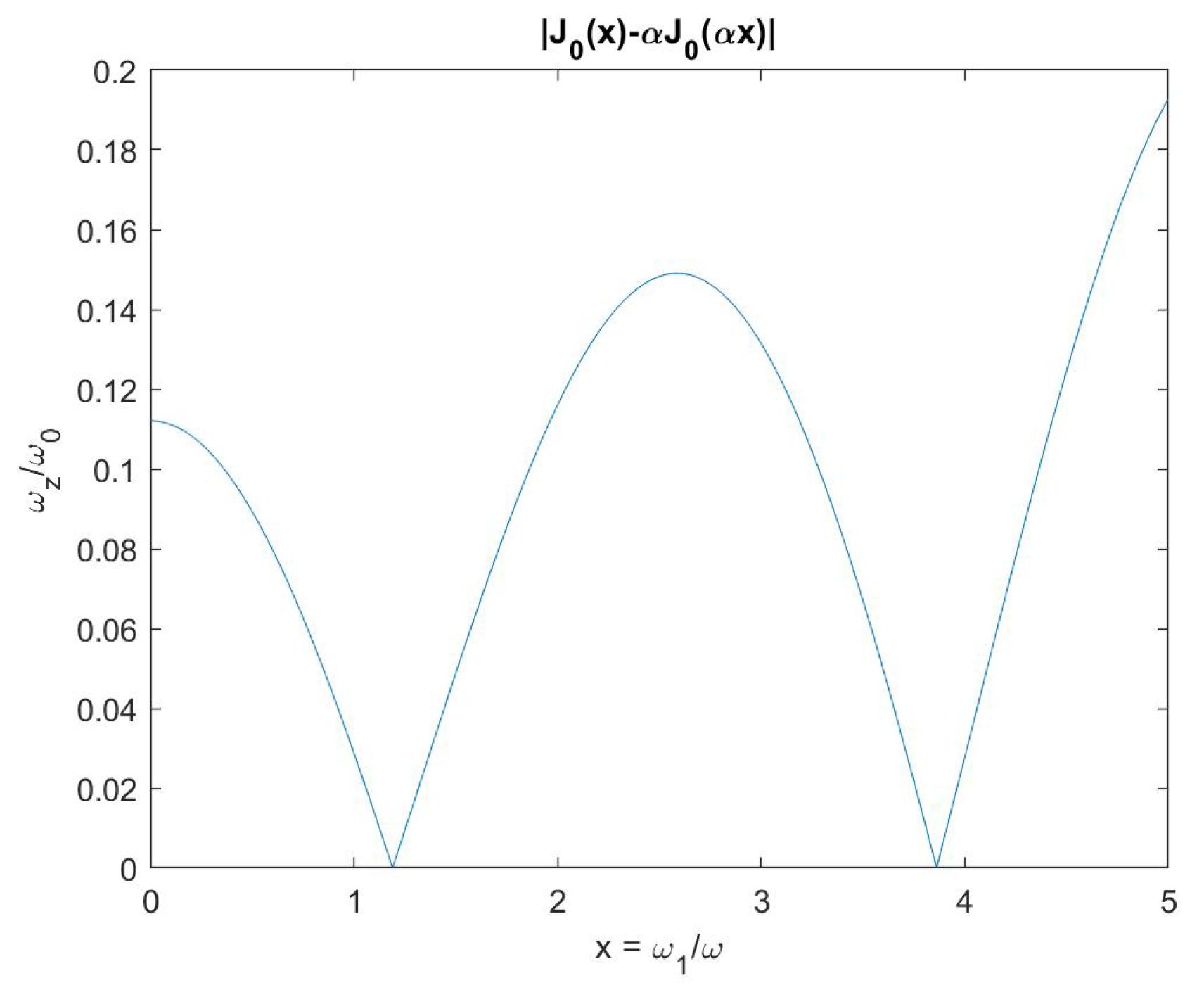
is shown in
Figure 18 and the absolute value of the critical dressing condition is shown in
Figure 19.
The first zero is at the critical dressing point the experiment will use because the nEDM term gets diluted by the Bessel function correction so the largest value of
should be used. This solution in the
approximation is
. When I performed simulations where I solved for
using the same field parameters as the experiment (
mG,
), critical dressing was at
. This 0.55% difference between my simulation value and the analytical
approximation value was the first indication that something was missing. The second indication was when I tried modulating the dressing field. When the dressing field is set for critical dressing, the neutrons and Helium precess about the z-axis at the same rate. Since dressing is controlling the relative rate, a change in
x has the effect, when averaged over, of producing a
about the z-axis between the UCN and
3He. The Bessel function is asymmetric about critical dressing so I will label the
’s as
and
where I will write
as
going forward since there will be two different magnitudes of the dressing field. Intuitively,
being near the magnitude of
should give symmetry about critical dressing. This would make sense since the UCN and
3He need to alternate relative phase shifts in a symmetric manner while
itself is asymmetric as mentioned. The data I looked at for symmetry was the scintillation signal which the experiment relies on. This signal is maximum when there’s a maximum component of anti-parallel spins between the two species (Appendix D talks about the spin dependent scattering length of of neutron-
3He capture which leads to a periodic scintillation rate and a pseudomagnetic field). Therefore, observing the behavior of
with modulation gives evidence as to whether the modulation is doing a good enough job to offset the pseudomagnetic field. But what I first saw was that
was leading to large asymmetries in
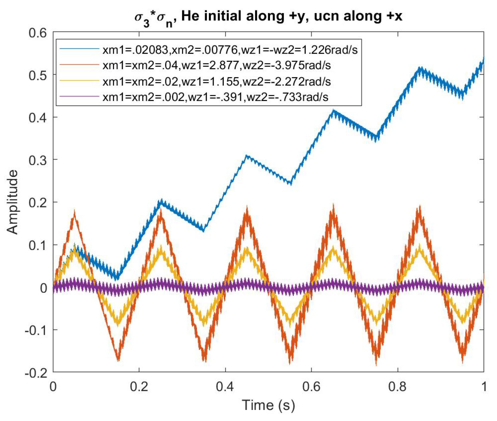
as shown in
Figure 20.
Note, in most of my simulations, the initial conditions have the spin parallel to each other. However
Figure 20 has the spins initially perpendicular so that the symmetry or asymmetry about 0 can be seen easier. As can be seen, the blue curve which had
, was asymmetric about 0 and therefore continuously had phase shifts building. Whereas the three other curves for
are mostly symmetric about 0. What this points to given the definition of
is that the expressions for
are wrong. This can be conceptualized by thinking about why symmetric
is leading to
symmetry. Looking at
Figure 19, symmetric
(
) for
small should lead to
. But as can be seen in the legend of
Figure 20,
and
have large percentage differences. This led me to think back to whether the
approximation is valid for
and the idea of extending the eigenvalues to higher orders.
6. Corrections to the Eigenvalues
The general expression for the second order correction to the eigenvalues is

and using the bar eigenstates of
where

Next are the third order corrections to the eigenvalues which I suspected to be the source. The third order corrections to the eigenvalues have two summation terms and one is easier to calculate than the other. The general expression is

Defining
, the third order correction in this context is

The Physics Reports [
1] made the approximation that the first term, which is more complicated than the second, is equal in magnitude as the second term and therefore did not calculate it. What I found is that the first term is actually larger than the second term and when included in the critical dressing condition, produces much better convergence with simulation values. The calculation for the second term in Equation 50 is

such that for different
q’s,
or
. The terms up to
are
so that the result is
For the calculation of the first term in Equation 50, first I would like to consider the terms that contain
since they will be similar in magnitude to the result in Equation 53. The only way to get a
in the first term is for
which means
(but with
) giving
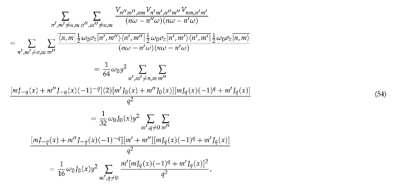
where the sum over
made
or else the whole term vanishes. Continuing the calculation of just the sum
The summation over
is simply a summation of
and
. Then substituting
as before, the final result for the first term in Equation 50 is
The new critical dressing condition is
Now, going back to the other terms that do not include
, they will either vanish when summed over or be quite small. An example is shown in Appendix E.
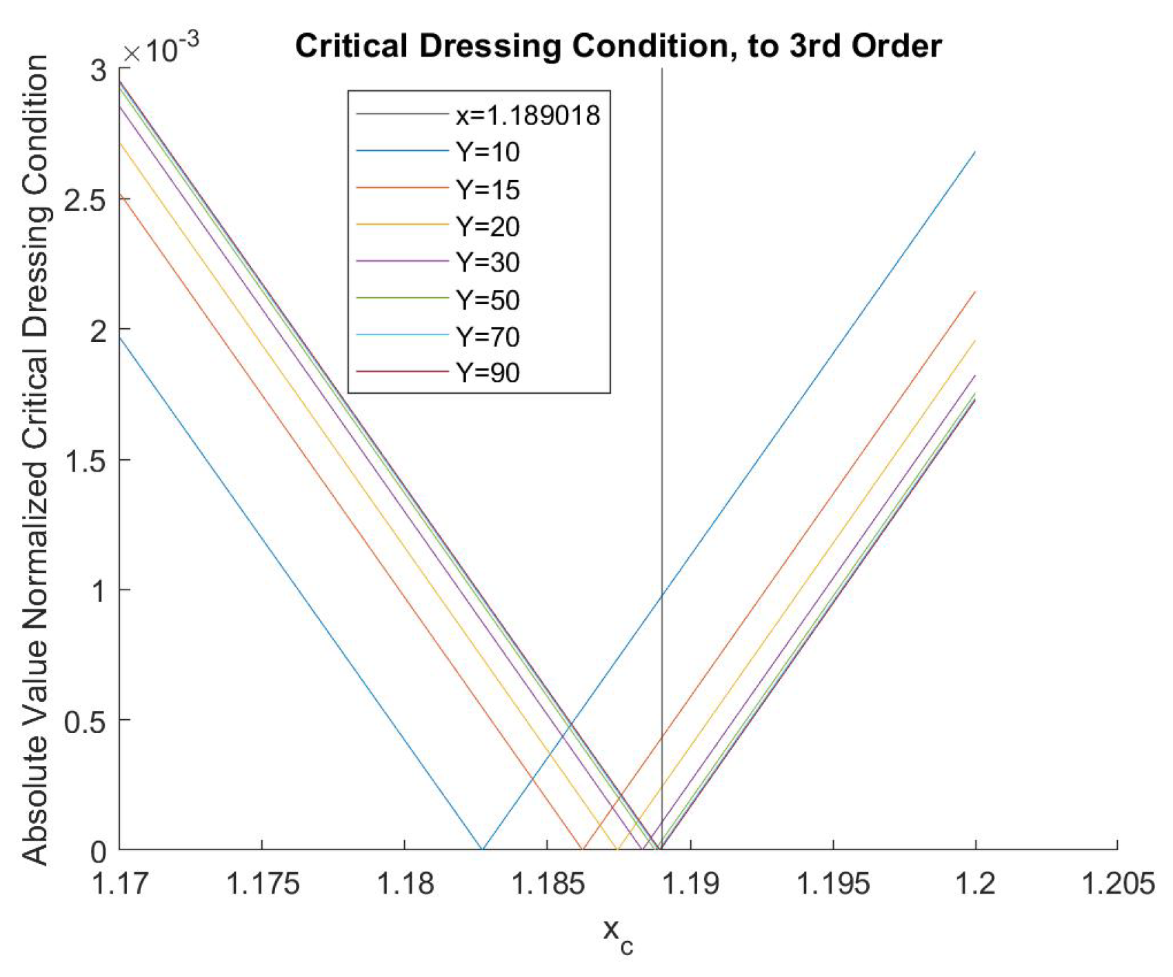
Figure 21 shows the zoomed-in view of the new critical dressing condition and how varies for different values of y. This demonstrates how the nEDM experiments needs to account for this shift in not only for the sake of critical dressing and modulating the dressing field but for an accurate expression for the scintillation rate. This third order correction also dilutes the nEDM signal.
What I now see from my simulations is much better agreement between my simulation
and the analytical expression for
that includes the third order corrections.
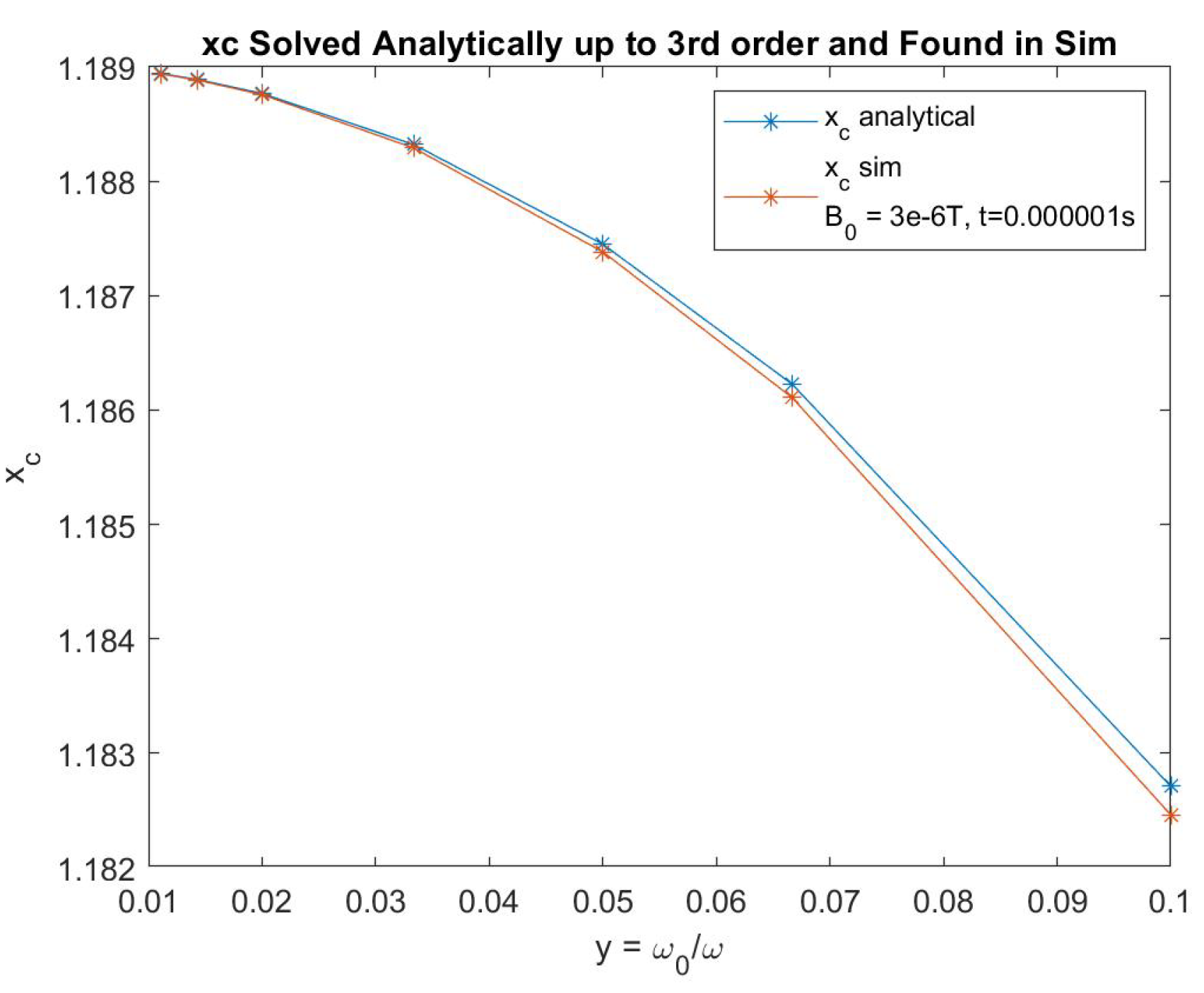
Figure 22 shows the analytical and simulation critical dressing parameters for different values of y. And
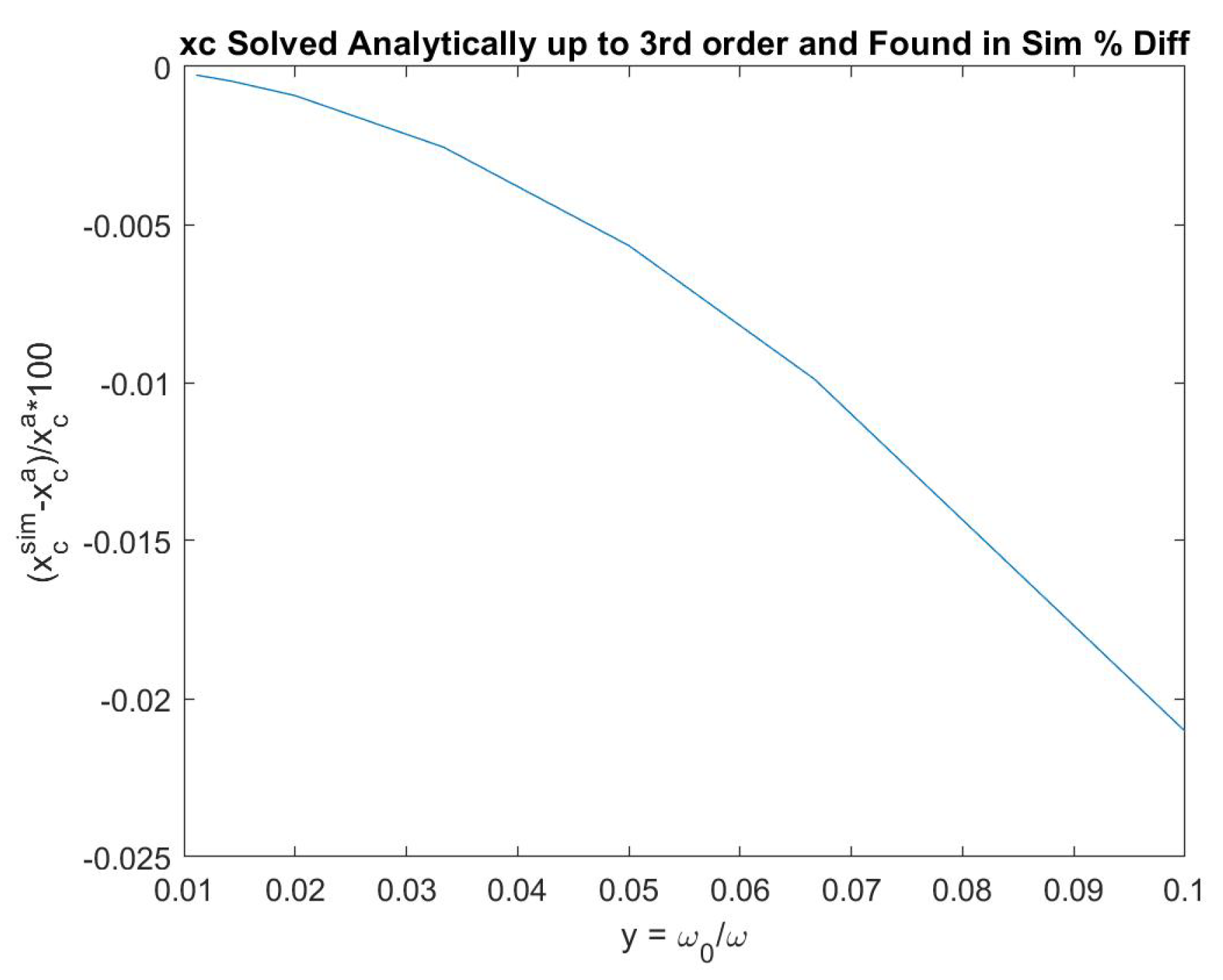
Figure 23 shows the percentage difference of these values at each given value of y. There is still a
dependence in
Figure 23 because the third order correction terms I’ve ignored are of course still proportional to
. Given I now have an accurate expression for the critical dressing condition, I can more accurately modulate around it.
7. Modulation and the Pseudomagnetic Field
With the third order corrections from the last section, I will briefly show what modulation looks like with a pseudomagnetic field on and off.
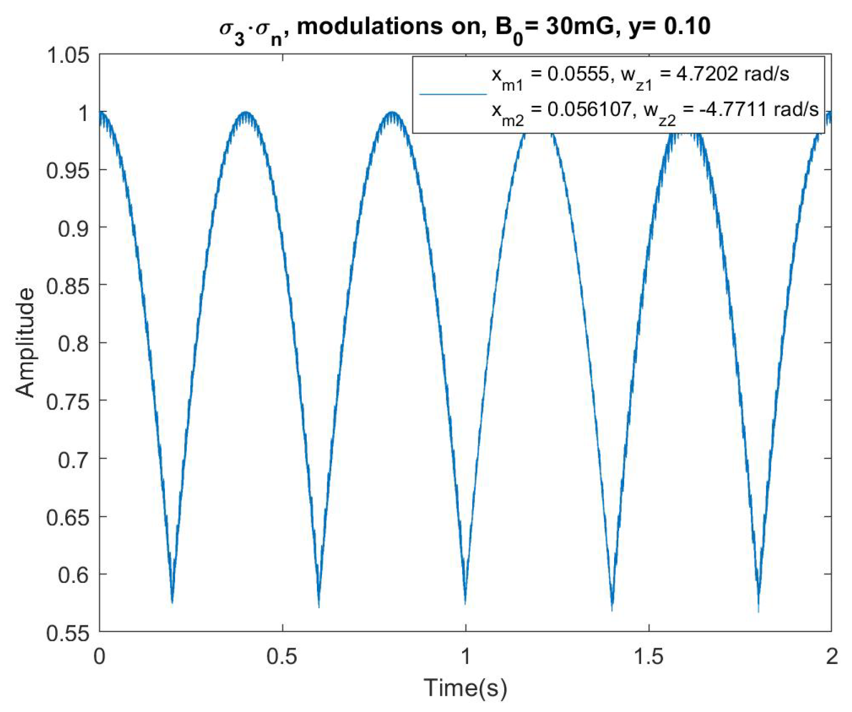
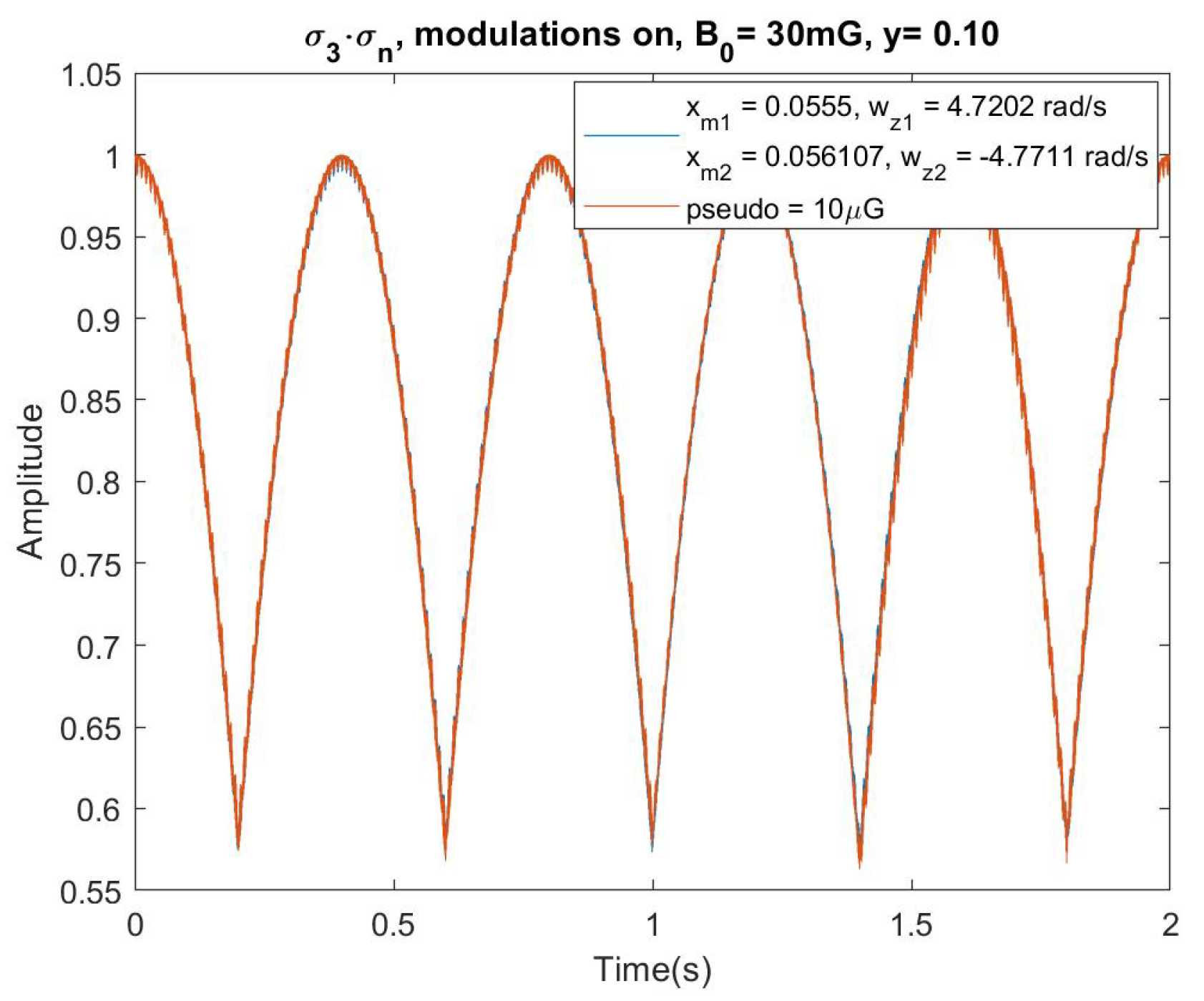
Figure 24 shows a near symmetric scintillation signals with modulation on and an applied pseudomagnetic field off.
As seen in the legend, the corrected do have magnitudes much closer to each other than before.
For the magnitude of
, I wanted to use the value from the paper by Leung et al.[
3] where for
and
such that
G. However, this magnitude is very small compared to the fields already present and the sensitivity of the simulation so instead I looked at
. The relevant plots are shown in
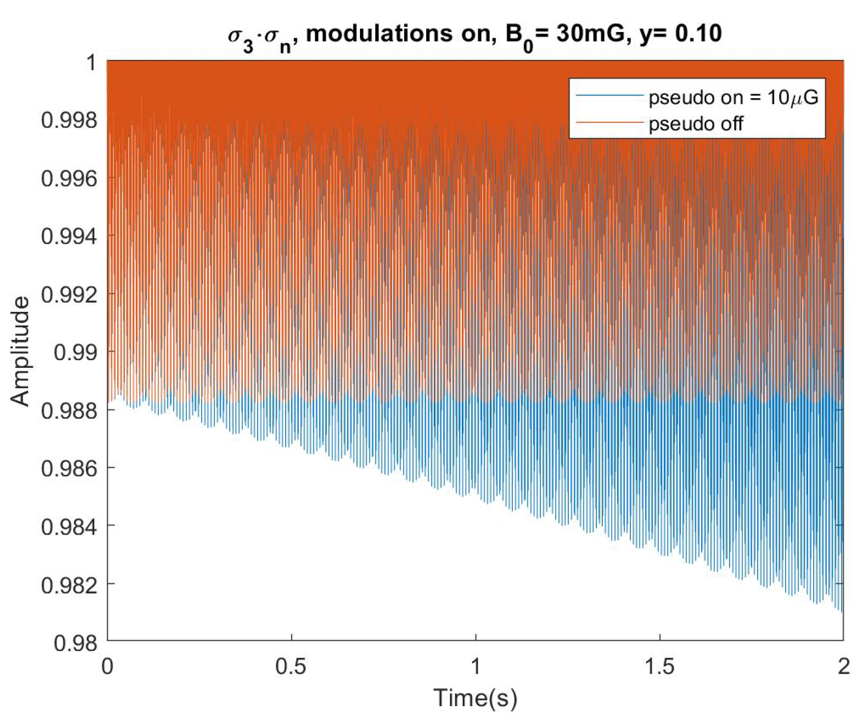
Figure 25 to 27. For a benchmark, I first show the difference in
for the pseudomagnetic field off and on without modulation. Followed by plots where modulation will cancel out the effects from
. Note that in
Figure 25, I chose to use the color blue for the pseudomagnetic field on and orange for it off which differs from other plots. This was solely to give a better contrast to the naked eye.
Figure 25 showed that
was inducing a non-negligible phase shift between the
3He and UCN that grows linear in time (with no modulation). Then
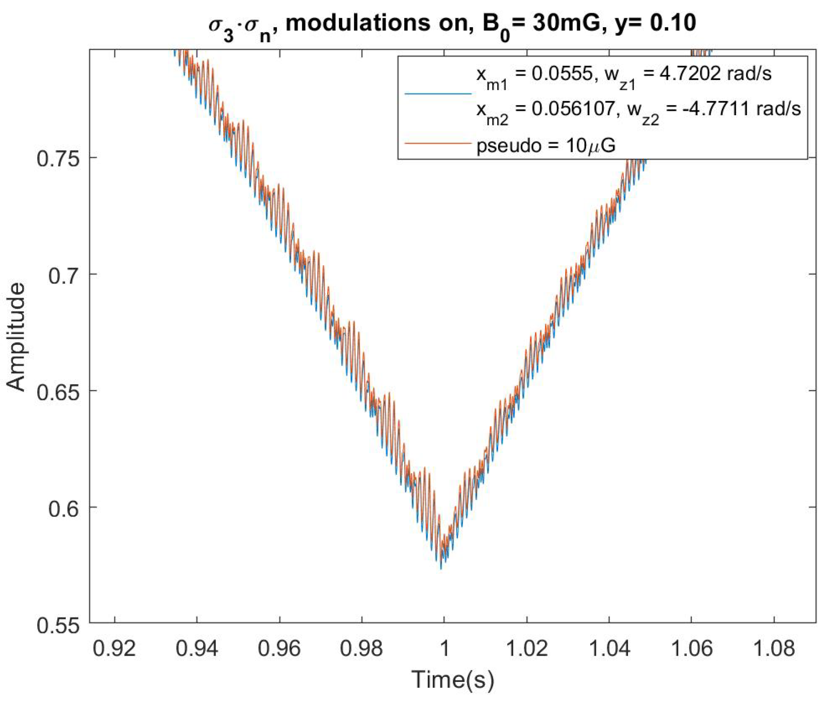
Figure 26 and 27 show the modulation doing a good job at canceling the phase difference that was built in the plots without modulation.
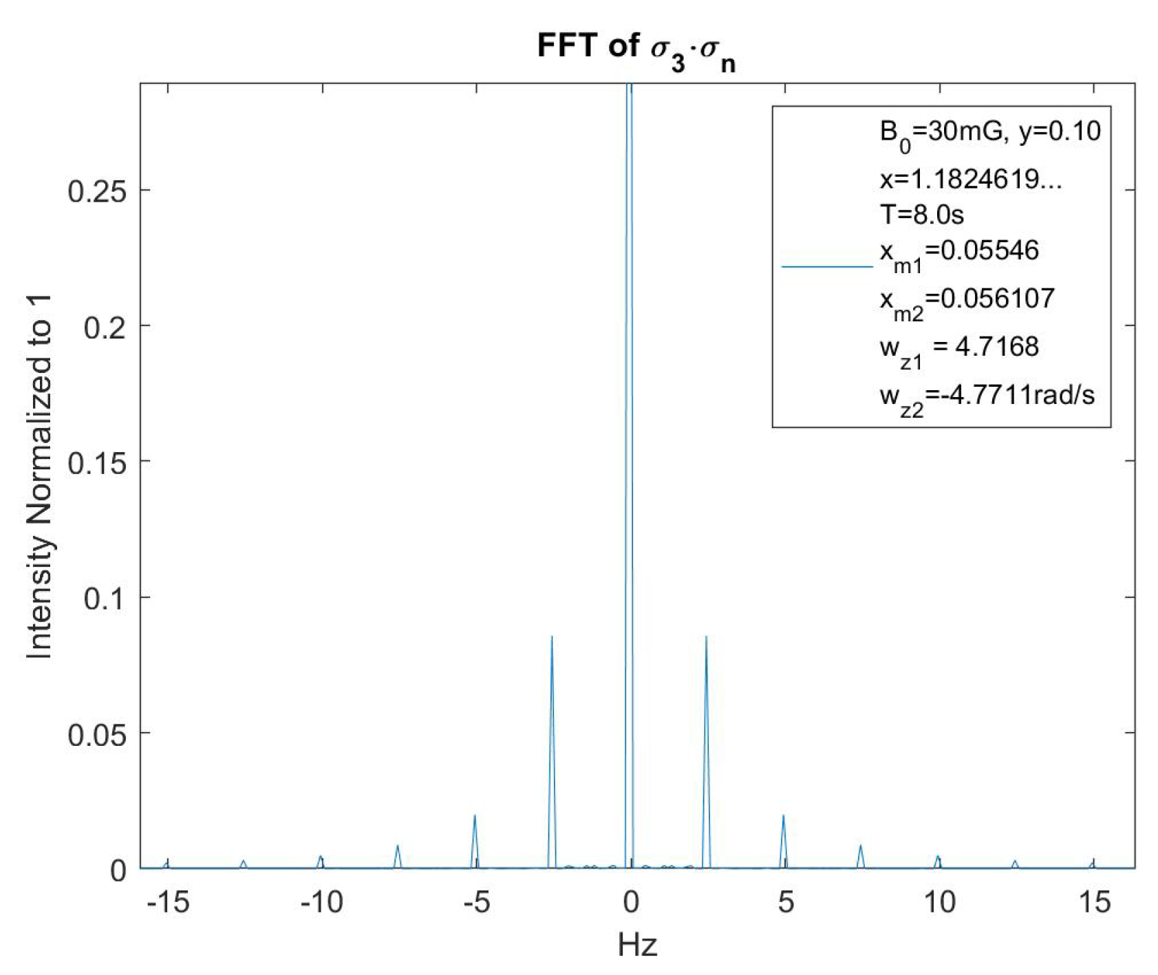
Finally, one way which Robert Golub proposed to quantitatively check how the modulations were performing was to check the relationship between the first and second harmonic signals in Fourier space. The idea is that the first harmonic at 1.25 Hz should be near zero if the modulations are symmetric about
. Whereas the second harmonic will have a much larger height and increase in height as the first harmonic signal decreases. So checking the ratio of the second to the first harmonic with modulation on pseudomagnetic field off and modulation on pseudomagnetic field on, will be a better test of whether the modulations are doing their job. I optimized symmetry by looping through
values that produced the lowest first harmonic signal. The results were
and
, close to the values I’ve been using and I used a simulation time of 8 seconds.
Figure 28 shows the FFT of
with modulations, no pseudomagnetic field and zoomed on the modulation harmonics.
The FFTs are shows in
Figure 29 where I zoomed-in on the harmonics but further zoomed-in on the first (1.25 Hz) and second (2.5 Hz) harmonics. The colors have been changed to better see where the curves differ and overlap.
The black curve for when the pseudomagnetic field is on has a larger value at the first harmonic which is expected. Due to the binning of the frequency axis which comes from the time steps and length of the simulation, there was no value exactly on 1.25 Hz or 2.5 Hz. For the 1.25 Hz, I took the average of the values at 1.1875 Hz and 1.3125 Hz. For the 2.5 Hz, I used the value at 2.4375 Hz. The results were that the ratio of the second harmonic signal to the first with the pseudomagnetic field off was 30.055. The ratio with the pseudomagnetic field on was 13.346. Thus, the pseudomagnetic field being flipped to on changed the relative ratios by about a factor of 2.25. This change is a good benchmark as to how well the modulations are doing going forward and with a field that is not 100x the experiment’s strength.
Figure 1.
3He in red and UCN in blue, the two critically dressed for 0.20s of simulation time.
Figure 1.
3He in red and UCN in blue, the two critically dressed for 0.20s of simulation time.
Figure 2.
for , frequencies solved for using the RK4 method. and are frequencies not currently included in theory.
Figure 2.
for , frequencies solved for using the RK4 method. and are frequencies not currently included in theory.
Figure 3.
for , frequencies solved for using the RK4 method. and are frequencies not currently included in theory.
Figure 3.
for , frequencies solved for using the RK4 method. and are frequencies not currently included in theory.
Figure 4.
for , frequencies solved for using the RK4 method. and are frequencies not currently included in theory.
Figure 4.
for , frequencies solved for using the RK4 method. and are frequencies not currently included in theory.
Figure 5.
for , frequencies solved for using the RK4 method. and are frequencies not currently included in theory.
Figure 5.
for , frequencies solved for using the RK4 method. and are frequencies not currently included in theory.
Figure 6.
for , frequencies solved for using the RK4 method. and are frequencies not currently included in theory.
Figure 6.
for , frequencies solved for using the RK4 method. and are frequencies not currently included in theory.
Figure 7.
heights vs y using the RK4. Intensity ranges from 36 to 4031
Figure 7.
heights vs y using the RK4. Intensity ranges from 36 to 4031
Figure 8.
heights vs y using the RK4. Intensity ranges from 370 to 4304.
Figure 8.
heights vs y using the RK4. Intensity ranges from 370 to 4304.
Figure 9.
and heights vs y using the RK4. Intensity ranges from 4050 to 41863 and 6861 to 68212 respectively.
Figure 9.
and heights vs y using the RK4. Intensity ranges from 4050 to 41863 and 6861 to 68212 respectively.
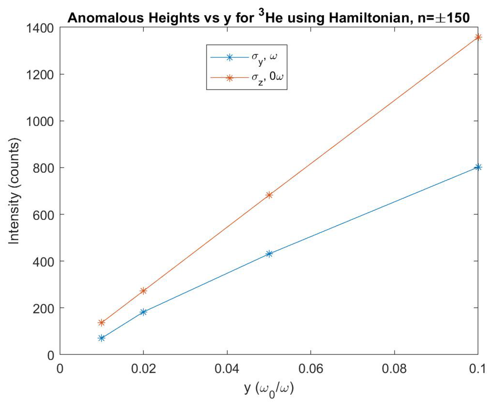
Figure 14.
and y vs. frequency peaks, solved using the Hamiltonian method for .
Figure 14.
and y vs. frequency peaks, solved using the Hamiltonian method for .
Figure 15.
for , frequencies solved for using the RK4 method. The frequencies are now accounted for with the first order corrections to the eigenstates. The bottom plot shows the anomalies with a zoomed-in view.
Figure 15.
for , frequencies solved for using the RK4 method. The frequencies are now accounted for with the first order corrections to the eigenstates. The bottom plot shows the anomalies with a zoomed-in view.
Figure 16.
for , frequencies solved for using the RK4 method. The and frequencies are now accounted for with the first order corrections to the eigenstates. The bottom plot shows the anomalies with a zoomed-in view.
Figure 16.
for , frequencies solved for using the RK4 method. The and frequencies are now accounted for with the first order corrections to the eigenstates. The bottom plot shows the anomalies with a zoomed-in view.
Figure 17.
for , frequencies solved for using the RK4 method. The and frequencies are now accounted for with the first order corrections to the eigenstates. The bottom plot shows the anomalies with a zoomed-in view.
Figure 17.
for , frequencies solved for using the RK4 method. The and frequencies are now accounted for with the first order corrections to the eigenstates. The bottom plot shows the anomalies with a zoomed-in view.
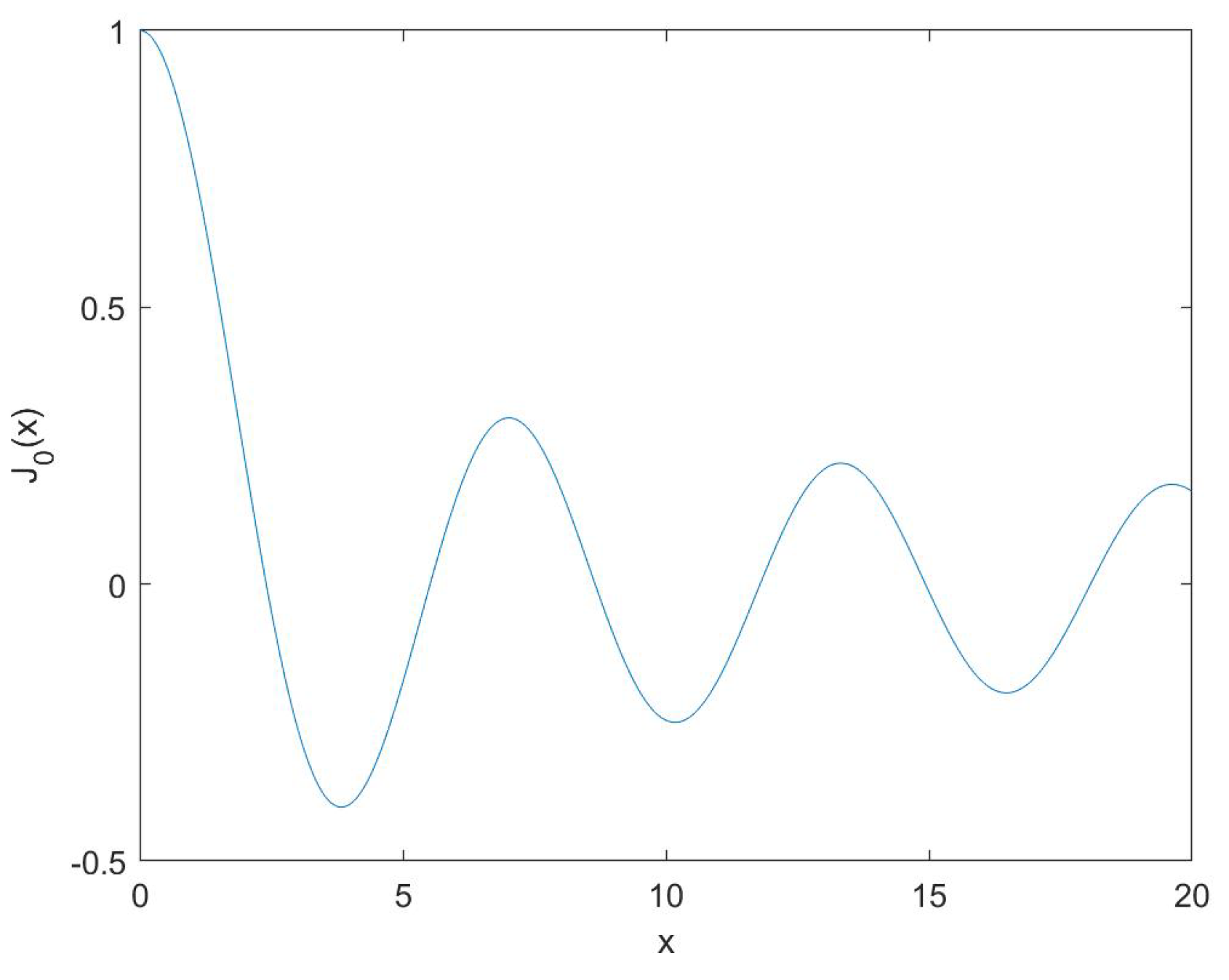
Figure 18.
The zeroth order Bessel function of the first kind.
Figure 18.
The zeroth order Bessel function of the first kind.
Figure 19.
The absolute value of the critical dressing condition where the y-axis is the relative frequency between UCN and 3He, , divided by .
Figure 19.
The absolute value of the critical dressing condition where the y-axis is the relative frequency between UCN and 3He, , divided by .
Figure 20.
vs time with in blue and in orange, yellow and purple. The two cases are mutually exclusive.
Figure 20.
vs time with in blue and in orange, yellow and purple. The two cases are mutually exclusive.
Figure 21.
Solutions for critical dressing parameters for different with the third order corrections as part of the condition. The first line in the legend is just a vertical line for , the solution for critical dressing in the approximation.
Figure 21.
Solutions for critical dressing parameters for different with the third order corrections as part of the condition. The first line in the legend is just a vertical line for , the solution for critical dressing in the approximation.
Figure 22.
Comparing the analytical critical dressing parameters from
Figure 5.12 to those found using the RK4 simulations.
Figure 22.
Comparing the analytical critical dressing parameters from
Figure 5.12 to those found using the RK4 simulations.
Figure 23.
The percentage difference between points in
Figure 5.13 for a given
Y.
Figure 23.
The percentage difference between points in
Figure 5.13 for a given
Y.
Figure 24.
vs time for modulation parameters and . The scintillation signals are more symmetric than any other modulated plot I have shown.
Figure 24.
vs time for modulation parameters and . The scintillation signals are more symmetric than any other modulated plot I have shown.
Figure 25.
vs time for no modulation and the pseudomagnetic field off (orange) and on (blue). The magnitude of is about 100 times larger than in the experiment.
Figure 25.
vs time for no modulation and the pseudomagnetic field off (orange) and on (blue). The magnitude of is about 100 times larger than in the experiment.
Figure 26.
vs time with modulation and the pseudomagnetic field off (blue) and on (orange). The magnitude of is about 100 times larger than in the experiment.
Figure 26.
vs time with modulation and the pseudomagnetic field off (blue) and on (orange). The magnitude of is about 100 times larger than in the experiment.
Figure 27.
A zoomed-in view of
Figure 26 near 1.0 s.
Figure 27.
A zoomed-in view of
Figure 26 near 1.0 s.
Figure 28.
The FFT of with modulation, zoomed-in on the harmonics.
Figure 28.
The FFT of with modulation, zoomed-in on the harmonics.
Figure 29.
The first and second harmonics. Their ratios are an indicator of how well modulation is working.
Figure 29.
The first and second harmonics. Their ratios are an indicator of how well modulation is working.
 where is an eigenstate of with eigenvalue and for a spin 1/2 particle, . Going forward, I will express states at or . |n> is an eigenstate of with eigenvalue n. and its definition starts from the energy density of magnetic field given as such that where .
 where and is an equivalent form of the eigenvectors shown in Appendix A for spin along +z and -z (). Going forward, I will write as m and any spin states with a + or - is a state in the x basis.
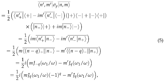 so that the expectation value is
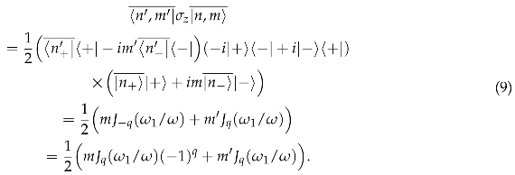 So that the expectation value is
 So that the expectation value is
 where and . Additionally, I can write the Hamiltonian matrix in the x or nbar basis but for my simulations, I used the z basis.
 The first term on the right hand side are the eigenstates whereas the second term is the 1st order correction.
 The first order correction is generally written as
 and so first order corrections to unprimed and primed states are
 where I define A as
 where I define as
 And similarly, a state up to first order is
 where the first two terms in the brackets are the usual zeroth order, unperturbed terms and refers to terms proportional to that I will ignore. Then, the expectation value is
 So that the expectation value up to y is
 so that the expectation value is
 and using the bar eigenstates of where
  Next are the third order corrections to the eigenvalues which I suspected to be the source. The third order corrections to the eigenvalues have two summation terms and one is easier to calculate than the other. The general expression is
 Defining , the third order correction in this context is
 The Physics Reports [1] made the approximation that the first term, which is more complicated than the second, is equal in magnitude as the second term and therefore did not calculate it. What I found is that the first term is actually larger than the second term and when included in the critical dressing condition, produces much better convergence with simulation values. The calculation for the second term in Equation 50 is
 such that for different q’s, or . The terms up to are
 where the sum over made or else the whole term vanishes. Continuing the calculation of just the sum
 where . From applying the creation and annihilation operators, you can see the only non-zero result is when so that . Assume and , then

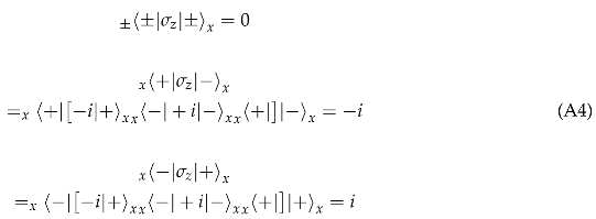

 The two cases above will yield the following terms
