1. Introduction
Linearity: there is a proportionality between input and output in the system. This means that there is an explainable relationship between the rate of change of the input and the rate of change of the output. To explain it mathematically: while the elements in the input set change additively; if the elements in the output set change additively, there is a linear relationship between input and output [
1] The function given in Equation (1) is a linear function. If we look at
Table 1, the total difference between input and output can be easily seen.
Most real-world problems do not have such a linear relationship and cannot be expressed in such systems. The relationships between the inputs and outputs of this type of problems often have a non-linear relationship. For this reason, the change between input and output cannot be expressed as additive or multiplicative (exponential functions).
Especially engineering, astronomy, mathematics, physics, etc. including in areas; In all branches of science, analyzing nonlinear systems is a problem. In this respect, it has created a very serious field of research. It has been accepted to linearize some systems under certain conditions or to try to solve them by considering them linear and to develop algorithms for this. This approach brings much convenience in practice. However, at the point where technology has come, trying to solve dynamic systems by linearizing them or assuming them to be linear does not give correct results in work areas that require high accuracy such as aerospace and defense industry technology, robotics, space research, and bioinformatics [
2] or it results in not achieving any results at all. Sometimes, although nearly accurate results can be obtained, it significantly prolongs the solution time. Depending on the size of the data processed, this time may be much longer than expected.
Since classical optimization techniques are generally inadequate in solving nonlinear systems, researchers have tried to produce different solution techniques [
3]. In this field, artificial intelligence algorithms have begun to be widely used in solving nonlinear systems. Although there is no universally accepted definition of artificial intelligence, according to the OECD, artificial intelligence is defined as the ability of machine systems to acquire knowledge, apply it and display intelligent behavior [
4].
Another definition is: Artificial intelligence: It is a computer discipline that focuses on self-managing (autonomous) algorithms or computer software that has the capacity to think, act and learn independently [
5].
Artificial intelligence natural language processing, problem solving, planning, perception, learning, adaptation, action, etc. It is the field of science and engineering that deals with the theory and practice of developing systems that exhibit the characteristics inherent in human behavior that we associate with intelligence [
6].
1.1. Meta-Heuristic Methods
Most real-world problems are nonlinear in nature, require serious computational costs, and have many complex solution areas. Therefore, optimization techniques, often called mathematical programming approaches or meta-heuristic methods, have been proposed to solve these problems [
7].
Meta-heuristic methods are also methods that enable us to find solutions more quickly in cases where we can find solutions using classical methods, but where the solution time may be very long. More than 500 meta-heuristic methods have been developed to date, and more than 350 of them have emerged in the last decade. Meta-heuristic methods are methods that produce reasonable solutions to optimization problems through trial and error. Intelligence is found in many systems other than humans, such as animals, microorganisms, ants, bees and other living creatures. Meta-heuristic methods have been the inspiration for many meta-heuristic methods, called nature-inspired algorithms [
8]. Evolutionary algorithms, physics-based algorithms, swarm-based algorithms, and human-based algorithms are the four most studied types of meta-heuristic algorithms [
9]. There are many popular meta-heuristic methods such as genetic algorithm, particle swarm optimization algorithm, gray wolf algorithm, whale optimization algorithm.
Table 2 shows examples of new meta-heuristic methods studied in recent years.
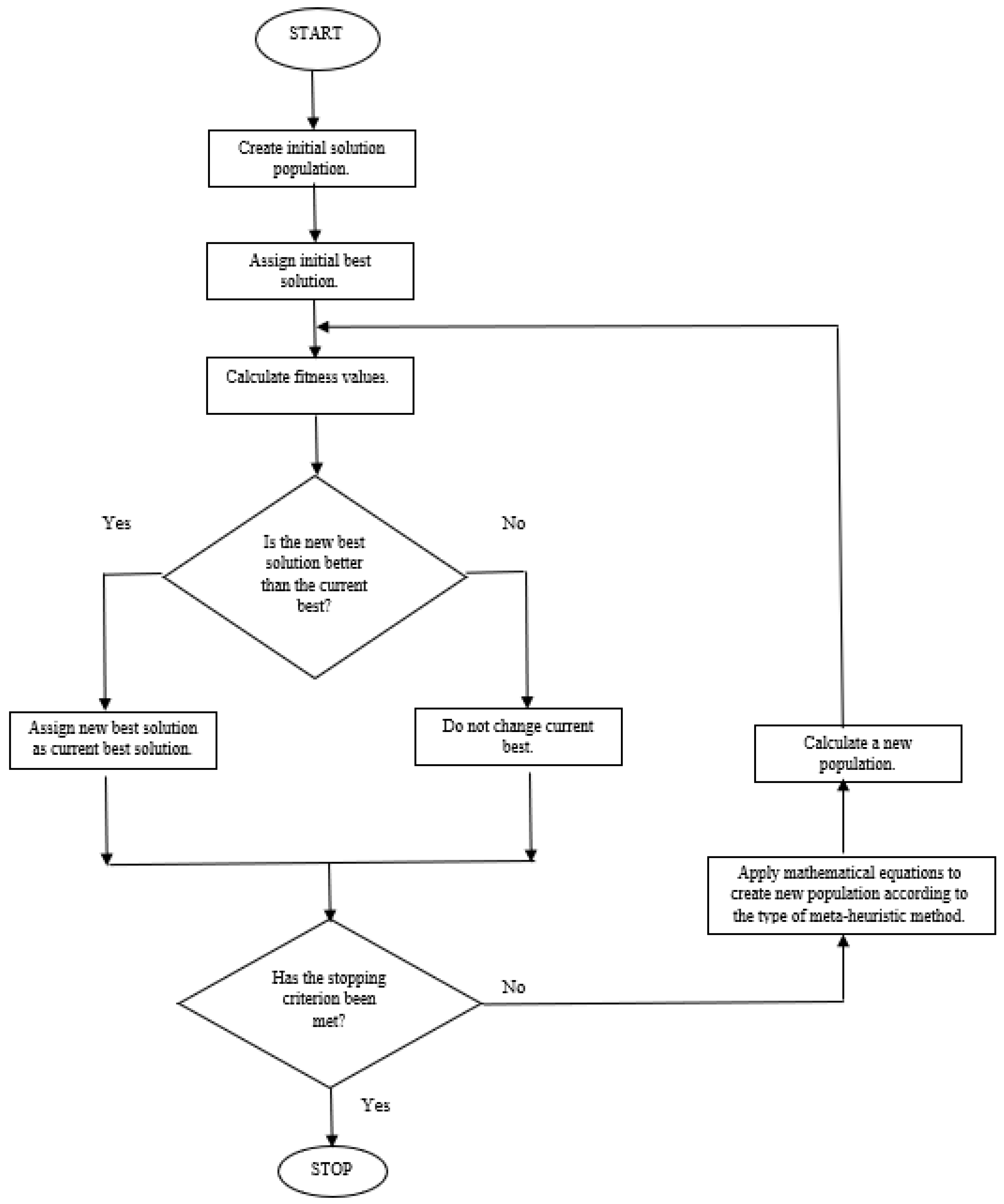
The general working principle of meta-heuristic methods is shown in
Figure 1.
The most effective part of a meta-heuristic method is the mathematical equations it uses when generating a new population. In fact, the most fundamental difference in each meta-heuristic method from the other is this mathematical infrastructure.
A meta-heuristic method initially creates a population of solutions, as shown in
Figure 1. It then calculates the value of each candidate solution based on their suitability for the solution. If the desired solution is reached, the algorithm terminates. Otherwise, it uses the meta-heuristic algorithm's own mathematical equations to generate new solutions. It reproduces the solution population, and the process is repeated.
1.2. Pi Number
Pi (π) is the 16th letter in the Greek alphabet and the first letter of the Greek word meaning "environment (περίμετρον)". Many studies have been done to calculate the current value of the number π. These studies aimed to prove that pi is a rational number. In other words, it is aimed for pi to repeat its previous values after one step and thus to understand that pi is rational [
31].
However, Swiss scientist Lambert proved that pi is an irrational number. In other words, he proved that the circumference and diameter of a circle do not have a common measure. Although its approximate value is expressed as π ≈ 3.1416; to express its real value, an infinite number of steps that do not repeat periodically are needed.
In this study, a pi coefficient calculation was made based on the Monte-Carlo method used to calculate the value of pi number. In the developed metaheuristic method, the pi coefficient calculated by the Monte-Carlo method was used in the algorithm and the pi coefficient value was used in the production of new population solutions.
2. Literature Studies
The application area of heuristic methods is a very wide field of study. It can be used very effectively, especially in nonlinear systems. Since experimental studies on clustering were carried out in this study, studies in the literature that use heuristic clustering methods were investigated. Especially studies carried out in recent years are included. Studies between 2019 and 2024 were mentioned.
Hugo Schnoering et al. [
32], in their study; they carried out a study aiming to extract address groups belonging to the same entity in bitcoin blockchains using heuristic methods. Thus, clustering operations of addresses belonging to blockchains were carried out. With heuristic clustering, the number of entities is reduced. Resources are saved and computational complexity is reduced. The effects of the heuristic methods used were measured by comparing the initial number of entities and the final number of entities. An address reduction of at best 70% could be achieved.
Gao, C. et al. [
33], in their study, they proposed an improved self-adaptive logarithmic spiral path black hole algorithm (SLBHA). SLBHA innovatively introduces logarithmic spiral path and random vector path to Black Hole Algorithm (BHA). The algorithm uses a parameter to control randomness, which increases the local usage capability. Moreover, a self-adapting parameter is introduced to control the switching mechanism and maintain the algorithm's balance between exploration and exploitation. To verify the effectiveness of the algorithm, comparison experiments were conducted on 13 data sets using evaluation criteria including Folkes and Mallows as well as the Jaccard coefficient. The proposed methods are whale optimization algorithm (WOA), compound intensified firefly exploration algorithm (CIEFA), enhanced black hole algorithm (IBH), etc. It was compared with selected algorithms such as. Success rate was measured with different metrics such as Standard deviation, Jaccard coefficient and FM values instead of accuracy. In many of the 13 different data sets, the proposed method achieved better results than others.
Kumar, G., K. et al. [
34], in their study, they proposed an optimized meta-heuristic clustering-based privacy key agreement routing technique to solve Wireless Sensor Network (WSN) security problems. It aims to simultaneously improve network security and connectivity while reducing energy consumption (EC). In the proposed system, a gateway-based network is constructed to design a switch arrangement protocol that ensures confidentiality during communication. The proposed routing strategy involves creating clusters of sensor nodes (Sn) that facilitate efficient selection. The number of cluster heads (CHs) that prioritize nodes with minimal changes. This effectively solves the EC problem. A comprehensive performance evaluation is performed, considering improvements in energy efficiency, packet delivery rate (PDR), throughput, end-to-end delay (E2 delay), and EC. The proposed method also incorporates the butterfly optimization technique to improve security and enable encrypted and decrypted transmissions. Rather than offering an accuracy rate for clustering, the proposed method provided a significant improvement in values such as memory space for key storage, computation time, and packet delivery ratio.
Puri and Gupta [
35], in their study, they proposed Heuristic-mrkmedoids (H-mrk-medoids) clustering to handle linear time clustering of big data. Aggregating the data into pieces and optimizing the centroid is done in the map phase, and clustering is accomplished by optimizing the weighted centroid in the reduce phase. As the main contribution of the paper, mrk-medoids are optimally aligned by the Modified Squirrel Search Algorithm (M-SSA), which provides efficient clustering based on the fitness quality measure. The accuracy rate of the designed method is 99%, and the RMSE rate of the proposed approach is 0.393095%. The result of the proposed approach showed significant improvements in the efficiency of clustering compared to traditional linear time clustering models.
Youseef Alotaibi [
36], in his study; he proposed Tabu Search and K-Means based MHTSASM algorithm for data clustering. MHTSASM starts with a random initial solution. It obtains the neighbors of the current solution, called trial solutions, and updates the memory elements for each iteration. It also uses concentration and diversification strategies guided by memory elements to improve the search process. Therefore, a high-level Tabu Search algorithm with long-term memory elements is presented. The highest success rate of 89.2% was achieved in experimental studies.
Masoud Aghdasifam et al. [
37] in their study; they proposed an approach called top-down hierarchical clustering (TDHC) to modularize the hierarchical clustering system by using local and global search strategies. The algorithm obtains a tree structure as output. In the presented method, the tree created is applied with a fitness function using a branch and bound approach to determine appropriate levels. A hill climbing algorithm was also designed to improve the quality of the resulting modular structure. This local search algorithm is applied to the results of the genetic algorithm for neighbor search. As a result of the experimental studies, the highest success rate of 92% was achieved.
Mehran Memari et al. [
38] in their study; they examined the performance and accuracy of classical and metaheuristic clustering algorithms. In the study, a new probabilistic method using clustering algorithms was developed to deal with the uncertainties of smart grid parts such as the output power of wind turbines and photovoltaics. The proposed method has been applied to two realistic test systems. They achieved the highest success rate of 97.9% for classical clustering methods and 97.93% for heuristic methods.
D.Viswanathan et al. [
39] in their study; they conducted a clustering study to group sensor nodes to save power in wireless sensor networks. Cluster head is important to balance the load in wireless sensor networks. In this study, clustering study was carried out with the help of Soft C-means multi-objective metaheuristic Dragonfly Optimization (SCMMDO). The main goal of the SCMMDO method is to determine the ideal cluster head for effective data transmission in wireless sensor networks. Initially, nodes are randomly distributed. The soft c-means method places sensor nodes into clusters based on three factors. These factors are received signal strength, residual energy, and bandwidth availability. Then the cluster head is selected using multi-objective meta-heuristic dragonfly optimization. The success rate obtained in the experimental studies was 96%.
Gyanaranjan Shial et al. [
40] in their study; they presented a hybrid metaheuristic algorithm using gray wolf optimization (GWO) and JAYA algorithm for data clustering. The algorithm consists of three steps: The first step is the initialization of the population, the second step is the fitness calculation, and the third step is the sequential position update, fitness calculation and selection of good solution candidates for the next steps. Afterwards, the process is repeated until the stopping step. Clustering studies were conducted on 15 datasets obtained from the ICI machine learning data repository. As a result, the best success rate of 97.83% was achieved.
LNC. Prakash K. et al. [
41] in their study; they proposed a swimming-based optimization technique to solve the problem of local convergence of optimal clusters. This work proposes a tale approach for clustering data using the firefly algorithm. It is shown how the K-Means technique can be applied to determine the location of centroids for known initial cluster centers. It was later developed to refine centroids and clusters using firefly optimization. Two metrics stood out in this study. The most used performance metric in the literature is the accuracy value. However, in this study, a metric called puirty was used. As a result of the experimental studies, the best purity value was calculated as 85% and the best F-measure (f-score) was calculated as 82%.
Sambu Anitha et al. [
42] in their study; they presented a detailed performance analysis of different existing cluster-based routing techniques for energy efficiency and network lifetime in wireless sensor networks. The work mainly focused on metaheuristic optimization algorithms for cluster-based routing in wireless sensor networks. As a result of experimental studies conducted with 7 different heuristic optimization methods, the best success rate of 96.63% was achieved.
Muhammad Shakil et al. [
43] in their study; they used whale optimization algorithm which is a metaheuristic method to detect the type of attack known as DDoS attack. In the method they call WOA-DD, attack requests are clustered, and methods detected as attacks are tried to be blocked. The algorithm has been compared with several existing clustering algorithms. The proposed method clusters the samples in the dataset into two clusters based on attributes: attack and normal requests. When a new request arrives, the algorithm predicts whether it is an attack or normal by calculating the distance with the two calculated cluster centroids. In experimental studies, the proposed method could reach a success rate of 82.83%.
Parul Agarwal et al. [
44] in their study; they proposed a new metaheuristic algorithm based on density-based subspace clustering logic for clustering high-dimensional data. To overcome the disadvantages of classical methods, the proposed method S_FAD; It finds subspace clusters of various density using different parameters of the DBSCAN algorithm. A hybrid method is used and optimizes the parameters of the DBCAN algorithm and uses the concept of hashing to discover all sets of non-redundant subspaces. For this purpose, it uses the hash tables it has created. Rand index and F-score metrics were used to measure performance. In the literature, F-score is a more valid metric as a performance measure. In experimental studies, the F-score reached the highest value of 85%.
Guo et al. [
45] in their study; they proposed a new evolutionary state-based multi-objective periodic bacterial foraging optimization algorithm for data clustering (ES-NMPBFO. The proposed algorithm is used in two data clustering cases consisting of nine public benchmark datasets and four credit risk assessment datasets. made a comparison with five different algorithms on six validity indices. The best accuracy value of 95.24% was achieved in 13 different data sets.
Senouci et al. [
46] in their study; they proposed a new heuristic clustering algorithm called Hop-Clustering Algorithm on Road Side Unit (HCAR) for the Internet of Vehicles (IoV). The latter is responsible for performing the cluster formation phase based on a simple heuristic algorithm using graph theory concepts such as node degree and adjacency matrix. Additionally, HCAR uses a new mechanism to solve the problem of cluster head (CH) unavailability by selecting a secondary CH using a weighted mechanism. Additionally, HCAR takes care of the maintenance phase to maintain the stability and structure of the clusters. The study compared values such as cluster CM life time, CH cash number and cluster number with MOSIC and DM-CNF methods. Transmission rates are also presented at different speed values such as 100 m/s, 200m/s and 300m/s.
Khedr, A., M. et al. [
47] in their study; they proposed a clustering algorithm called Advanced Sparrow Search Algorithm for IoV (Internet of Vehicle) (ESSAIoV) which integrates genetic algorithm and Sparrow Search Algorithm. ESSAIoV can work in the IoV high mobility nodes scenario and produces clusters optimized for effective communication. It uses a fitness function that combines the benefits of weight-based and mobility-based clustering approaches. The fitness function used considers mobility measurements across the cluster distance to create the least number of clusters with stable CHs. Vehicle clustering is an effective way to improve communication ability between vehicles. In the study, the number of clusters and lifetime values were measured in trials conducted with 30, 40, 50 and 60 devices in areas of 1 km
2, 2 km
2, 3 km
2 and 4 km
2. The proposed method gave better results than other methods.
3. Material and Method
3.1. Innovative Aspects of This Study
This study has presented an application that has a high potential to bring a new field to the meta-heuristic methods literature. This new developed method proposes a new heuristic method, the pi algorithm, based on the Monte-Carlo method, which is one of the calculation techniques used to obtain the number pi. For this purpose, firstly the Monte-Carlo method and calculations regarding the production of pi number are mentioned. Then, the mathematical model of the newly proposed pi algorithm is presented.
No similar study has been found in the literature that imitates the calculation of the pi number and seeks solutions to problems in this way. There are studies on calculating pi number with the Monte-Carlo method. However, these studies are not studies in which the Monte-Carlo method is used as a heuristic method. No method has been found in the literature where this approach is presented as a meta-heuristic method. In this respect, this study is a first in the heuristic methods literature.
Additionally, many different heuristic methods have been used in experimental studies on data clustering. However, the fact that the pi algorithm is a method that has not been studied in the literature also makes its use for clustering original. Because no study has been found in the literature that combines the pi algorithm and clustering.
Considering all this, this study is a study that can make original contributions to both the heuristic methods literature and the clustering literature.
3.2. Monte-Carlo Method and Generation of Pi Number
Monte-Carlo method; We can define it as a method that uses random numbers and is used to perform statistical simulations [
48]. The Monte-Carlo method was discovered by Nicholas Constantine Metropolis [
49] and popularized by Stanislaw Ulam [
50].
If the inputs of the system are in an indefinite form and their distribution can be calculated with a function, the Monte-Carlo method can be used. It is used in many fields such as numerical analysis, molecular physics, nuclear physics, and simulation [
51]. Similarities between probabilistic calculations are used in problem solving. The Monte-Carlo method is also an important method in solving complex and multi-parameter systems [
52].
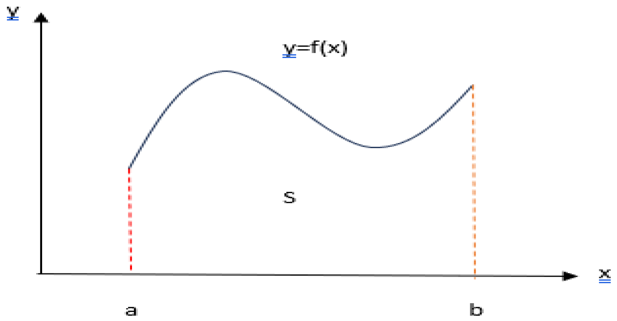
Numerical integration is the process of calculating the area under the curve of a function y=f(x) with certain boundaries.
Figure 2 represents numerical integration.
In Equation (2); The numbers a and b are constants and are the limits of the integral. If the function f(x) is continuous in this interval, the result of the integral is also constant. Its value is equal to the area under the y=f(x) curve and bounded by the lines x=a and x=b.
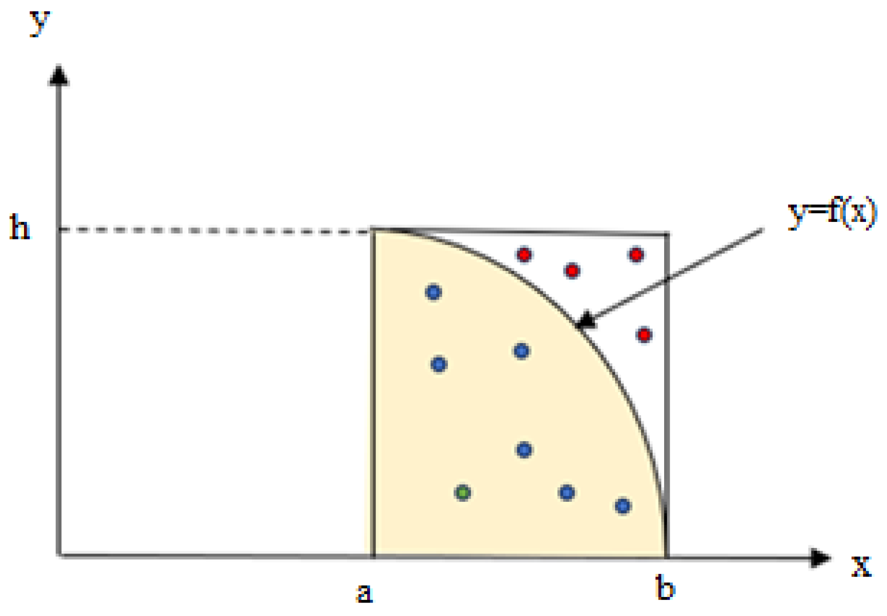
Monte-Carlo integration is a technique that integrates using random numbers. While different methods generally try to calculate the integral on a uniformly distributed grid; The Monte-Carlo method selects points randomly when calculating the integral. In the Monte-Carlo method, arbitrary combinations are generated to calculate the integral [
49]. Let's consider the integral of the function f(x) in the interval [a, b]. The application of the Monte-Carlo method is shown in
Figure 3.
In
Figure 3, there is a rectangle with corner coordinates [a,0] and [b, h]. The f(x) function divides this rectangle into two different regions. The first region is the region under the function who’s integral we want to calculate. The second region is the region at the top of the function. The coordinate pair, which will be randomly generated with a uniform distribution, is placed inside the rectangle. If the x coordinates of the points are chosen to remain in the [a, b] range and the y coordinates to remain in the [0, h] range; in this way, for each coordinate pair, it will be clear whether the point to be selected will be below or above the f(x) curve. The ratio of the number of points under the function (P
x) to the total number of points (P
t) will give an approximate expression of the ratio of the area under this function (A
x) to the area of the rectangle (A
t). Equation (3) shows this relationship.
For the integration calculation, two random numbers need to be generated. The first of these is for x in the range [a, b], and the other is for the y value in the range [0, h]. It is understood whether the number y is in the range [0, h] or not by comparing it with the number obtained from the f(x) function. If the randomly generated number is a number that falls in the shaded region, we use it in integration. If the y-f(x) value is zero or a negative value, it means that the random number falls in the shaded region. With this logic, many random numbers are generated; (x, y) pairs are obtained. In this way, values for integration are obtained. The resulting ratio will approximately give us the value we want to obtain.
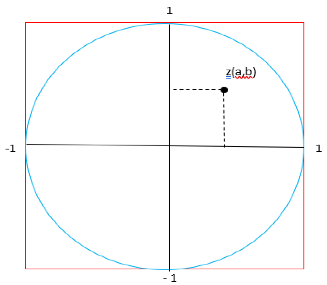
If we adapt the Monte-Carlo integration method to the process of counting the points falling into a circular region from random points with a uniform distribution in a square area, we obtain the relation in Equation (4) [
49].
Here, the value 1 is the radius of the unit circle. If we were to show this on a unit circle, it would look like
Figure 4.
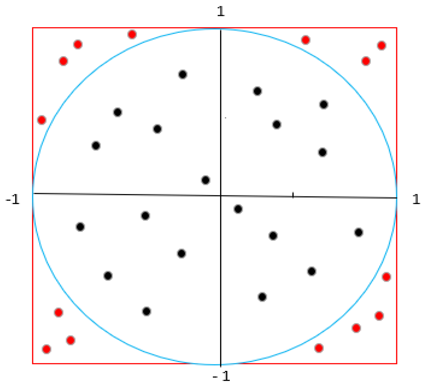
If we create random points inside the square with coordinates z (a, b), some of them will be inside the circle and some will be outside.
Figure 5 represents this.
If we ratio the probability of the shots falling inside the circle to the probability of them falling inside the square and multiplying this value by 4, we obtain the approximate value of the number π. This situation is shown in Equation (5).
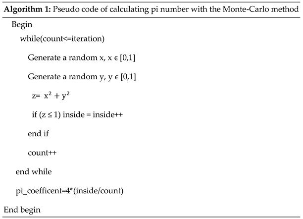
When the resulting value is multiplied by 4, the approximate value of the number π will be obtained. As the number of points is increased, a number closer to the desired value is obtained. The pseudo (rough) code of this method is given in Algorithm 1.

3.3. A New Metaheuristic Method: Pi Algorithm
In this section, the pi algorithm, and its related methods, developed as a new metaphysical method, are presented. In the previous section, it was mentioned how the pi number was generated using the Monte-Carlo method. In this section, a different pi coefficient was calculated for each feature to be produced using the Monte-Carlo method. This calculated pi coefficient was used to produce new solutions in the pi algorithm, which is the new metaheuristic method developed.
First, let's explain the method used to calculate a different pi coefficient for each attribute. The r value, which is the concept of radius in the unit circle mentioned in
Figure 4 and
Figure 5, is accepted as half of the minimum value and maximum value of an attribute in our new algorithm. Equation (6) shows this.
The attributei in the formula represents each measured attribute in the data set.
Just as the radius in a circle is half the diameter value; In our algorithm, half of the difference between the largest value and the smallest value of an attribute is accepted as the radius value of that attribute. A z value will be calculated according to the situation expressed in Equation (4). If this number produced remains less than 1, which is the radius of the unit circle, it will be considered to fall within the circle. Otherwise, it will be included in the area outside the circle. In the Pi algorithm, this formula has been updated as in Equation (7).
Thus, the random number to be generated is considered to remain within the circle if its radius is smaller than the r value. Here, the circle will be the data range that accepts the maximum value and half of the minimum value of the data attribute as a radius.
Euclidean distance measure was used as the distance measure in this study. The distance calculation used is given in Equation (8) [
53].
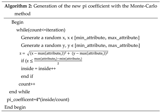
A pi coefficient will be calculated for each attribute. Therefore, the more parameters a data has, the more pi coefficients will be calculated for it. In Algorithm 1, the pseudo code for calculating the pi number with the Monte-Carlo method was given. The value of the new pi coefficient calculated in our newly developed algorithm will be shown in Algorithm 2.

Here, while calculating the value of z, the differences between the x and y values previously calculated in the Monte-Carlo method and the maximum value of the attribute in the data set were taken. Because the distance between the x and y values to be produced and the highest value of the attribute will be the limit values of the circle in both numbers. Therefore, when calculating the radius, both the maximum and minimum values were used; When calculating z, only the maximum value was used.
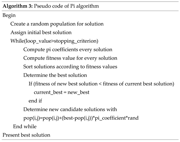
With the method proposed in Algorithm 2, pi coefficients are obtained to be studied in the ranges of each attribute for the data sets studied. In Algorithm 3, the pseudo code of the newly proposed pi algorithm is given.

The population is created by diversifying around the best element until the stopping criterion is met.
In this study, unlike other metaheuristic algorithms in the literature, pi coefficients were used. As new solutions were produced at each step, new pi coefficients for each attribute were calculated and new candidate solutions were created taking these coefficients into account. The part where we produce the new solutions specified in the rough code is given in Equation (9).
The main thing in metaheuristic methods is to produce values around the best solution. For this reason, the distance of the current value of the solution from the best solution is determined and diversified with the pi coefficient. A new solution value is calculated by applying the resulting value to the old solution. In this way, new solutions are obtained. The random value here is used to ensure solution diversity. Operations continue until a certain stopping criterion is met.
4. Data Clustering
Clustering is an analysis technique that tries to group objects according to the similarities of their attributes. This grouping process is done according to predetermined criteria [
54].
Clustering: Since it tries to group the similarity of objects to each other, it needs a measurement method that can determine whether the objects it evaluates are like each other. To determine this, two main types of measures are used, called distance measures and similarity measures [
55]. The distance measure used in this study is the Euclidean distance and is given in equation (8).
Machine learning algorithms are basically divided into three different areas: Supervised learning, unsupervised learning, and reinforcement learning. Supervised learning, a labeled training set is used for output. In this learning method, the data in the training set consists of binary input objects and output values in the form of a vector. Unsupervised learning, unlabeled data is used. Grouping is done based on the distance relationship between the attributes [
56]. In reinforcement learning, by giving penalties or rewards to software agents for the work they will perform; An attempt is made to help the child automatically decide on the behavior that is expected to be ideal. The reinforcement learning agent learns through its actions based on its experiences [
57].
Clustering is learning without a trainer. Because of this feature, it manages to find hidden patterns in the data. Therefore, it has been the subject of important research in many fields such as image processing, pattern recognition, signal processing, bioinformatics, and data mining [
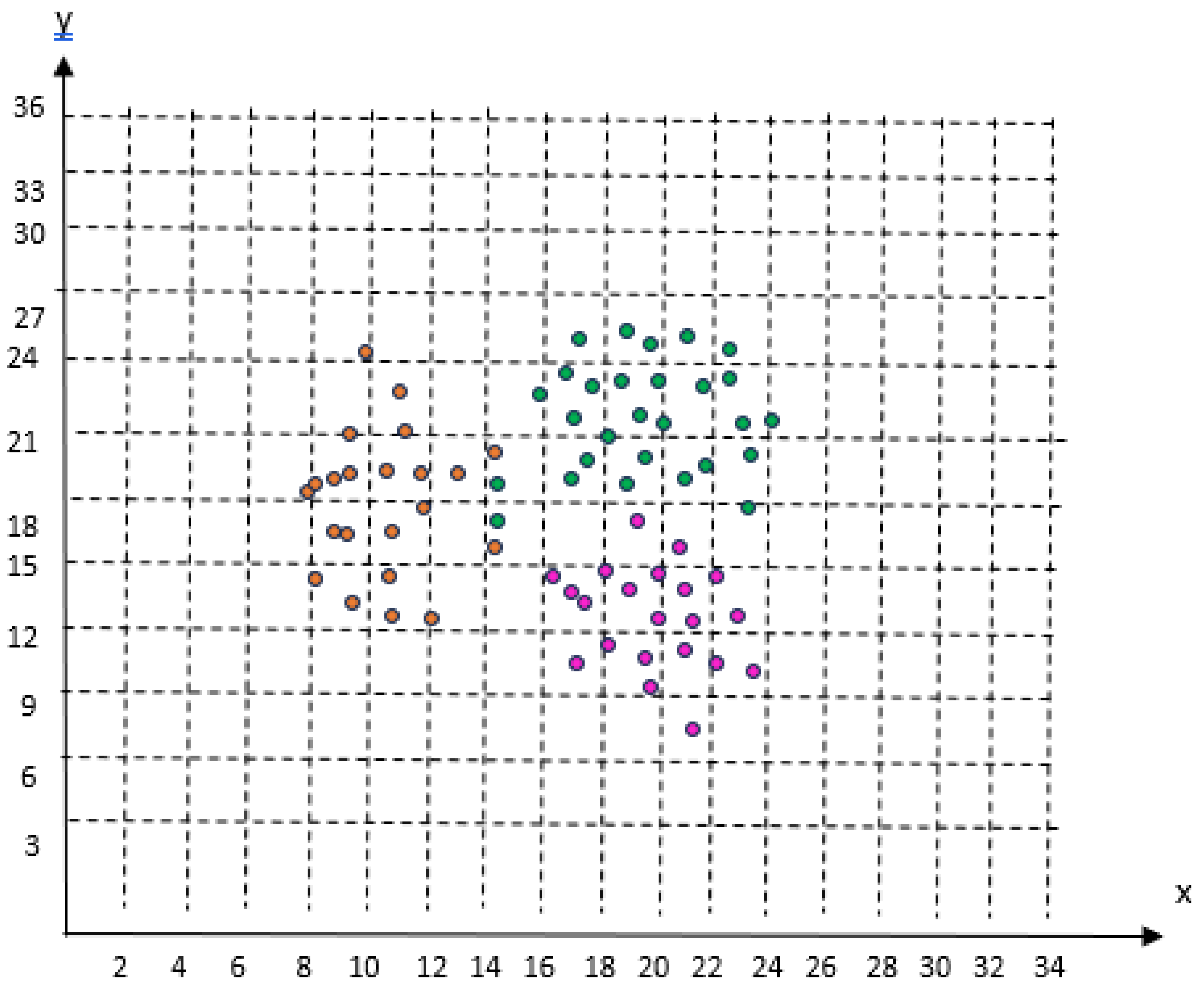
54]. A representative illustration of the clustering process is given in
Figure 6.
As represented in
Figure 6, each color represents a cluster. x represents one attribute and y represents the other attribute. The number of features is the number of parameters of the system and their number will vary depending on the problem to be solved. What is expected in clustering is that the groups are separated from each other as much as possible. In this case, data representing a point will be clearly included in a cluster. However, some data may be in more than one cluster. In this case, if it is not in the set, it should be in, it causes an error in terms of prediction.
4.1. Confusion Matrix and Performance Evaluation in Data Clustering
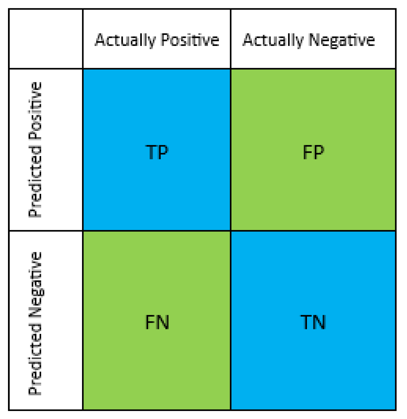
Confusion matrix is a matrix that represents the success of the applied model. Each cell of the matrix represents an evaluation factor. Factors are numerical information about the actual values to be obtained and the expected values to be estimated. The confusion matrix will be a nxn dimensional matrix. N is the number of clusters attempted to be predicted. There are four types of results in the confusion matrix. These:
True Positives (TP): It refers to the number of correctly predicted positive clusters/classes. It is also referred to as true positive.
True Negatives (TN): It refers to the number of correctly predicted negative clusters/classes. It is also expressed as true negative.
False Positives (FP): It refers to the number of incorrectly predicted positive clusters/classes. It is also referred to as false positive.
False Negatives (FN): It refers to the number of incorrectly predicted negative clusters/classes. It is also referred to as false negative [
58].
Based on these values, the confusion matrix is calculated. The confusion matrix for the two clusters is represented in
Figure 7.
The concepts of accuracy, precision, sensitivity (recall) and F1 score are used in the performance evaluation of the clustering process. Equations (10), (11), (12) and (13) show their formulas, respectively [
59].
Accuracy is the value resulting from the ratio of correctly predicted values to the total data set.
Precision is the ratio of values determined as true positives to the total positives.
Recall is the ratio of those detected as true positives to the sum of true positives and false negatives.
F1 score is the harmonic mean value of sensitivity and precision.
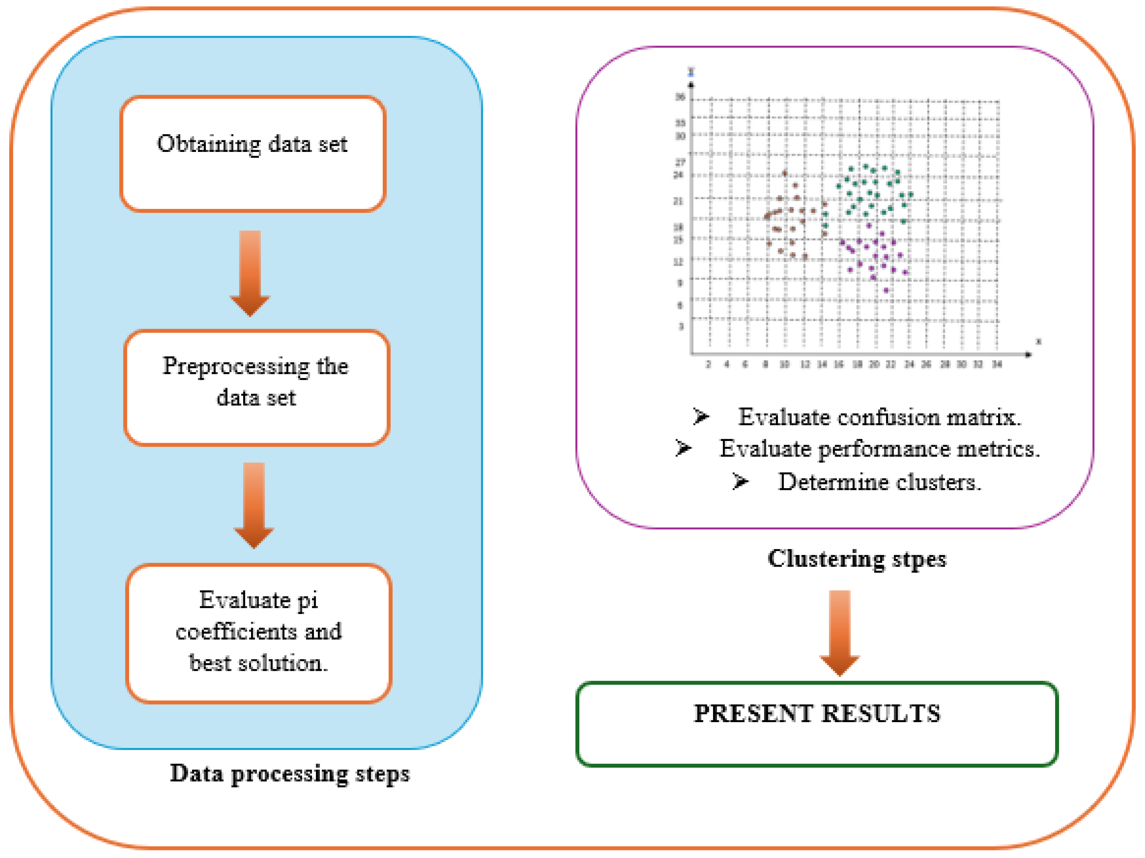
The general working principle of this study is given in
Figure 8.
5. Experimental Results
In this study, results were made on 5 different data sets. These are Iris, Occupancy Detection, Wisconsin Breast Cancer Original, Water Quality and Banknote Authentication datasets. In this section, the clustering results of the data sets with the pi algorithm proposed in this study are presented. Confusion matrixes for each data set were calculated. Accuracy, precision, sensitivity (recall) and F1 score performance values were calculated with the values obtained from the confusion matrix.
5.1. Iris Dataset Results
The Iris dataset [
60], obtained from the UCI Machine Learning Repository, is one of the most widely used datasets in clustering/classification methods in the literature. The dataset contains 3 classes of 50 samples each. Each class corresponds to one type of iris plant. 30 examples for each class were used to train the algorithm. For testing, 20 samples from each class, 60 in total, were allocated. Each instance consists of 4 attributes.
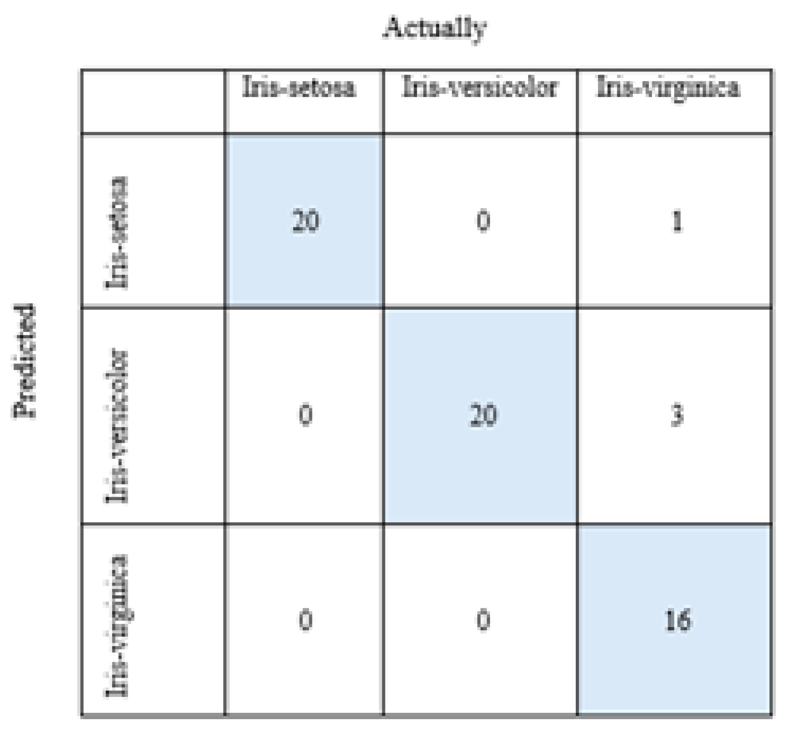
Figure 9 shows the confusion matrix obtained after the pi algorithm of the iris-plant data set.
One best matrix will be obtained from the Pi algorithm. This will be the optimum value that will perform the clustering process best. In this data set, 4 pi coefficients will be obtained. The values of the best matrix and pi coefficient matrix obtained are as in
Table 3.
Figure 9 shows the confusion matrix obtained after the pi algorithm of the Iris data set.
For the iris-setosa group TP=20, TN=20+0+3+16=39, FP=0+1=1, FN=0+0=0,
For the iris-versicolor group TP=20, TN=20+1+0+16=37, FP=0+3=3, FN=0+0=0,
For the iris-versicolor group TP=16, TN=20+0+0+20=40, FP=0+0=0, FN=3+1=4.
In this case, the results given in
Table 4 are obtained for the Iris-plant data set.
Accuracy is the most heuristic of performance measures. If the accuracy of the model we developed is high, it can be considered that the best performance criterion is accuracy. However, if the numbers of false positive and false negative values are significantly different, it is necessary to look at other parameters to measure the performance of the model [
61].
F1 score consists of the harmonic mean of precision and sensitivity. It considers both false positives and false negatives. Especially when the data has an uneven class distribution, looking at the F1 score is more useful than looking at the accuracy value [
61].
Looking at
Table 4, the accuracy value is higher between accuracy and F1 score. This shows that it would be more appropriate to choose the accuracy value as a performance criterion.
5.2. Occupancy Detection (OD) Dataset Results
The OD [
62] data set obtained from the UCI Machine Learning Repository is an application data set for energy saving. The energy used for heating, ventilation, and air conditioning; It is thought to save money by automatically adjusting it according to demand. For this reason, 5 different attributes are measured from the environment. The output data is 2 groups. There are 3 different files in the data set. It is divided into 1 training and 2 test sets. In fact, the attributes of input and output data are the same in all 3 files. In this study, from the training file containing 8143 samples, 100 samples were reserved for the first group and 100 samples were reserved for the second group.
The values of our best matrix and pi coefficient matrix obtained are as in
Table 5.
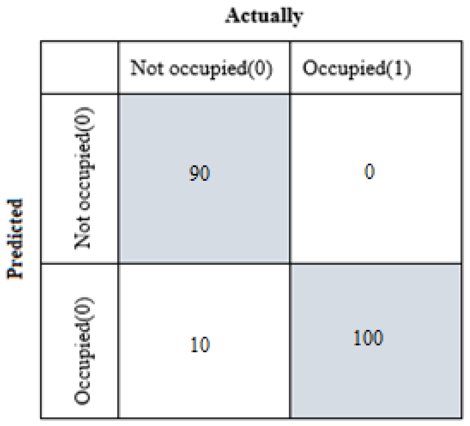
Figure 10 shows the confusion matrix obtained after the pi algorithm of the OD data set.
For the Not occupied group TP=90, TN=100, FP=0, FN=10,
For the Occupied group TP=100, TN=90, FP=10, FN=0.
In this case, the performance results in
Table 6 are obtained for the OD data set.
5.3. Wisconsin Breast Cancer Original (WBCO) Dataset Results
The WBCO [
63] dataset obtained from the UCI Machine Learning Repository is a dataset related to breast cancer. Grouping was made as benign or malignant. It consists of 699 samples in total. However, there are missing attributes in the data. After these are removed, 684 samples remain. 50 of these are benign and 50 are from the malignant group for testing. Each instance has 9 attributes. The values of the best matrix and pi coefficient matrix obtained are as in
Table 7.
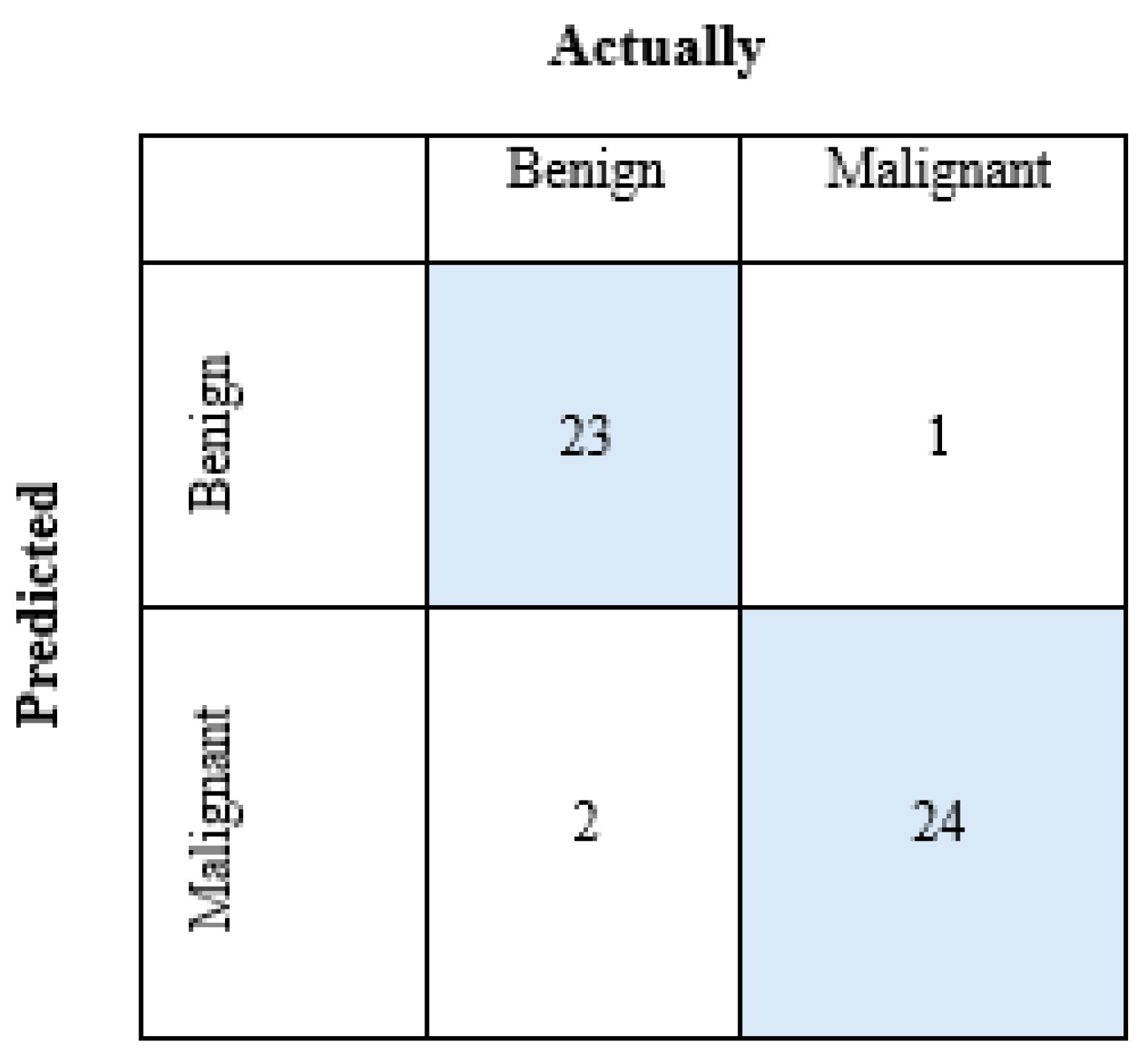
Figure 11 shows the confusion matrix obtained after the pi algorithm of the WBCO dataset.
For the benign group; TP=23, TN=24, FP=1, FN=2,
For the malignant group; TP=24, TN=23, FP=2, FN=1.
In this case, the performance results in
Table 8 are obtained for the WBCO data set.
5.4. Water Quality (WQ) Dataset Results
The dataset obtained from Kaggle [
64] is a dataset created from synthetic data on water quality in the urban environment. Of the data set consisting of a total of 7996 data, 100 samples from the safe group and 100 samples from the unsafe group were reserved for testing. There are 20 attributes for each instance. The values of the best matrix and pi coefficient matrix obtained are as in
Table 9.
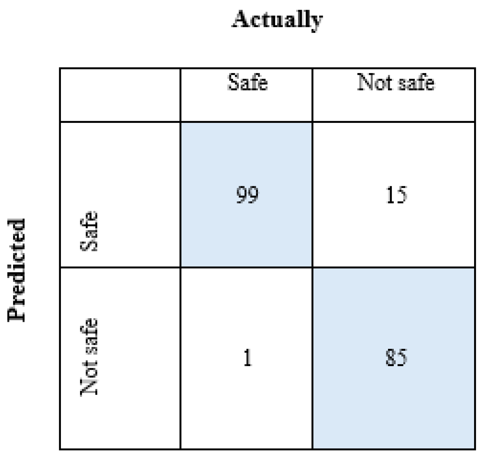
Figure 12 shows the confusion matrix obtained after the pi algorithm of the WQ data set.
For the Safe group; TP=99, TN=85, FP=15, FN=1,
For the not safe group; TP=85, TN=99, FP=1, FN=15.
In this case, the performance results in
Table 10 are obtained for the WBCO data set.
5.5. Banknote Authentication (BA) Dataset Results
The BA [
65] dataset obtained from the UCI Machine Learning Repository worked on images taken from genuine and forged banknote samples. Values were obtained using the wavelet transform method on the digitalized images of banknotes. The training data, consisting of a total of 1273 data, consists of 4 attributes. 50 samples were allocated for testing from each of 2 groups of data. The values of the best matrix and pi coefficient matrix obtained are as in
Table 11.
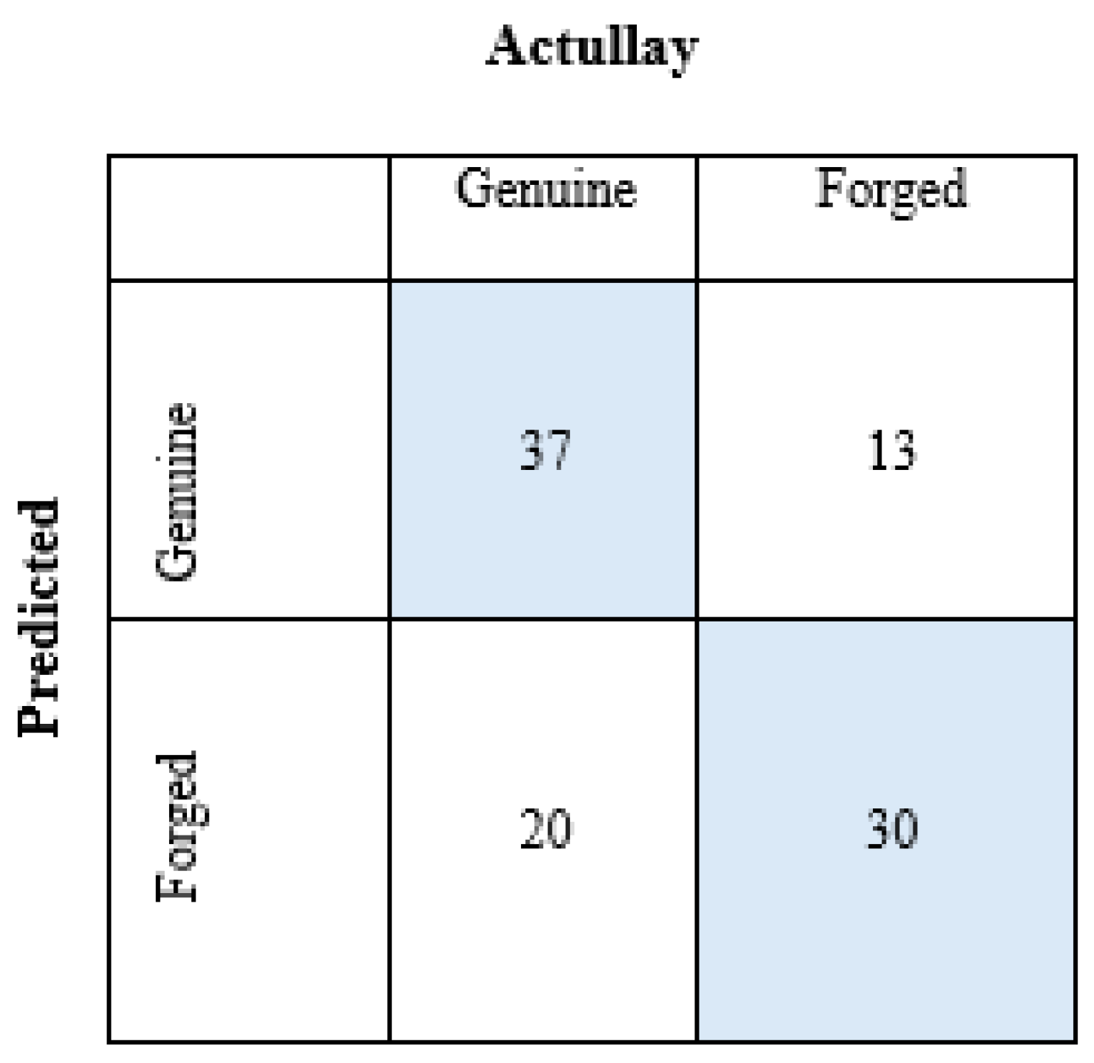
Figure 13 shows the confusion matrix obtained after the pi algorithm of the BA data set.
For the Genuine group; TP=37, TN=30, FP=13, FN=20,
For the Forged group; TP=30, TN=37, FP=20, FN=13.
In this case, the performance results in
Table 12 are obtained for the BA data set.
5.6. Comparison of Experimental Results
In this section, the experimental results of 5 different data sets used in the study are presented in
Table 13.
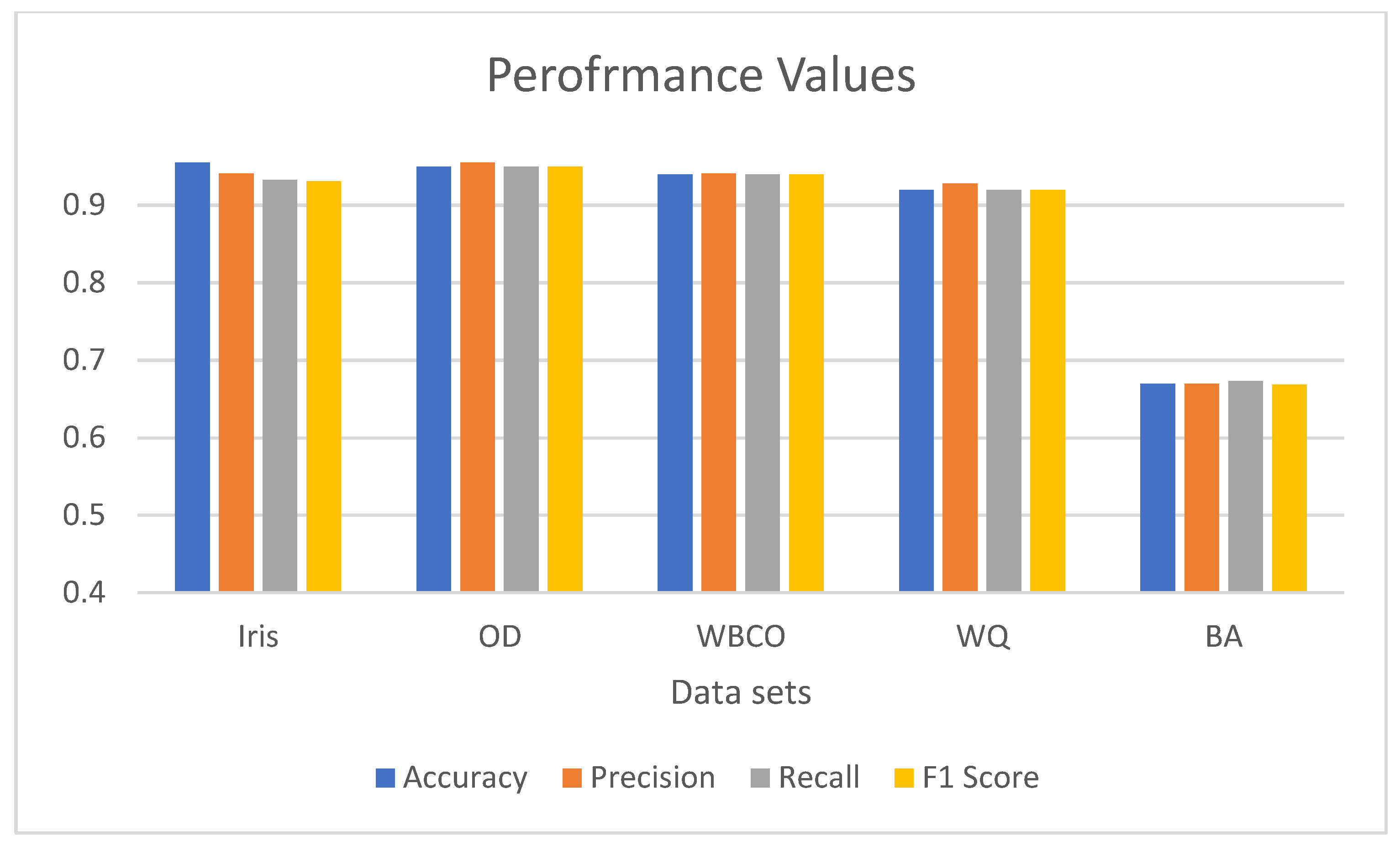
Table 13 shows the averages of accuracy, precision, recall and F1 score values for each 5 data sets.
In
Table 14, a comparison of the data sets on which experimental studies were conducted in this study, studies in the literature and the newly proposed pi algorithm are given. Since experimental studies were conducted on clustering, which is a learning method without an unsupervised, in this study, the success levels of clustering studies in the literature were taken as an example. There are many studies on these data sets in the literature. But most of these are studies on classification.
Table 14 presents a comparison of the data sets on which we conducted experimental studies with clustering studies.
When
Table 14 is examined; Although our proposed method is a new study and open to improvement, it is better than some of the success rates in the literature. Even where it is not the best, it is very close to other methods that are better than it. If we examine the study of Huang and Gel in
Table 14; rand index value was given as a criterion of success. Rand Index (Rand Coefficient) value already has the same formula as accuracy value.
6. Discussion
In this study, experimental studies were conducted on 5 different data sets. When the accuracy rates of the data sets are examined, the accuracy rates of the first 4 data sets are quite good; The results of the recently studied Banknote Authentication data set are lower than others.
The distribution of the attributes of the data set is very important in terms of accuracy. In cases where the means and variances of the features are significantly different from each other, the feature with large arithmetic means and variances are more effective on the others and significantly suppress the effects of other features [
78].
For this reason, some normalization applications are made to perform clustering analysis on the data more accurately. In the Z-score method, which is one of these and widely used in statistics, data is transformed into new values with an arithmetic mean of zero and a variance of one [
79]. In the Z-score method, normally distributed data with a certain range and measured on a proportional scale are standardized. The data is processed as shown in Equation (14) [
80].
Here is the attribute data,
is the average of the features,
shows the standard deviation of that attribute.
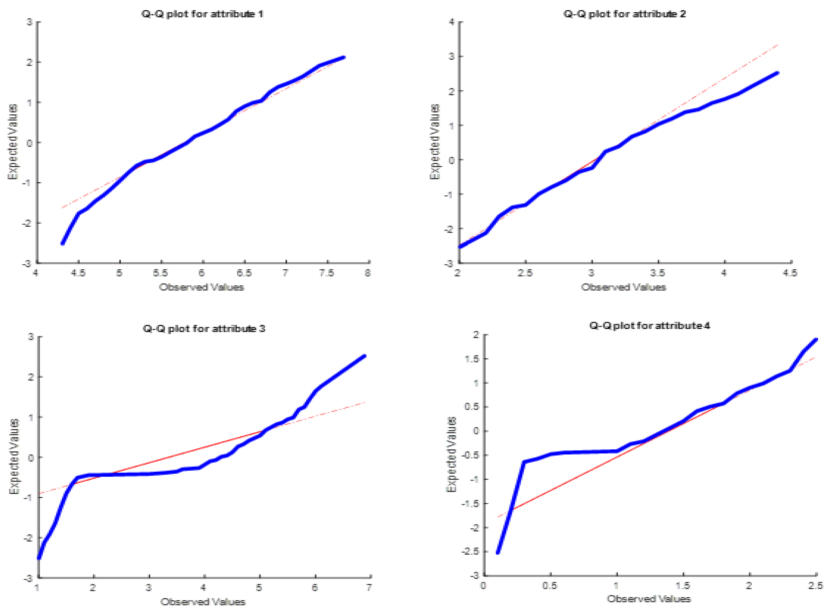
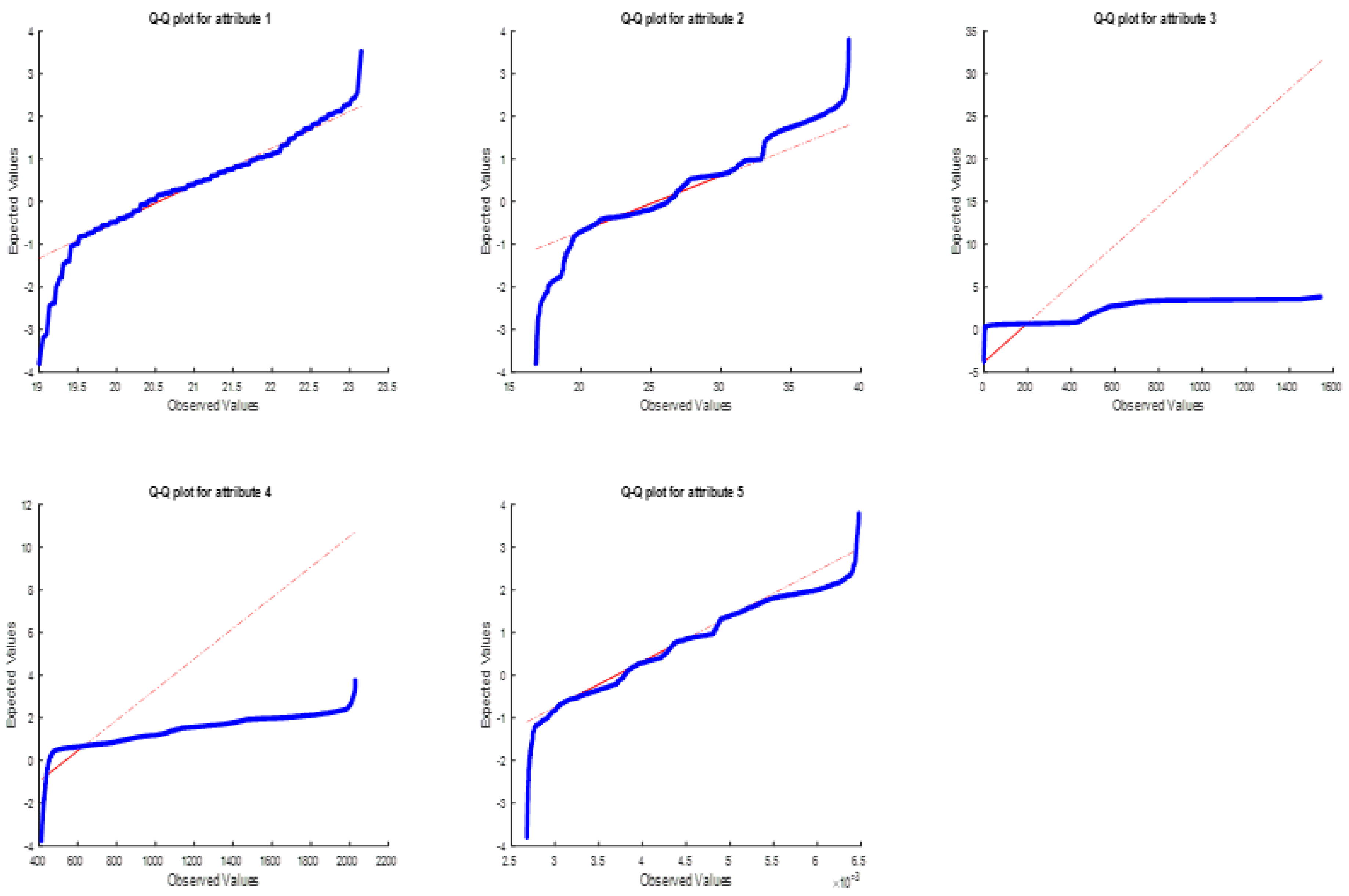
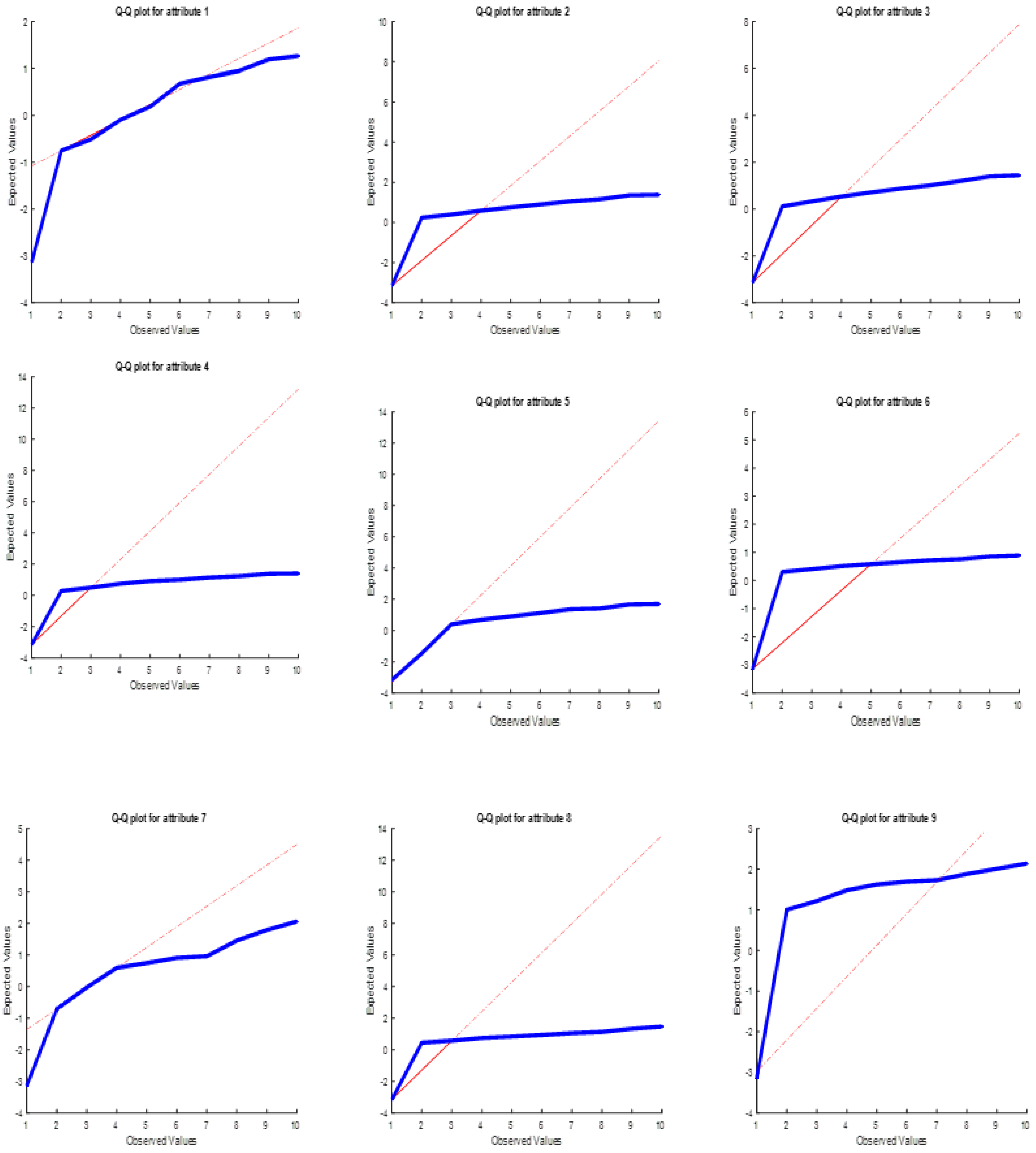
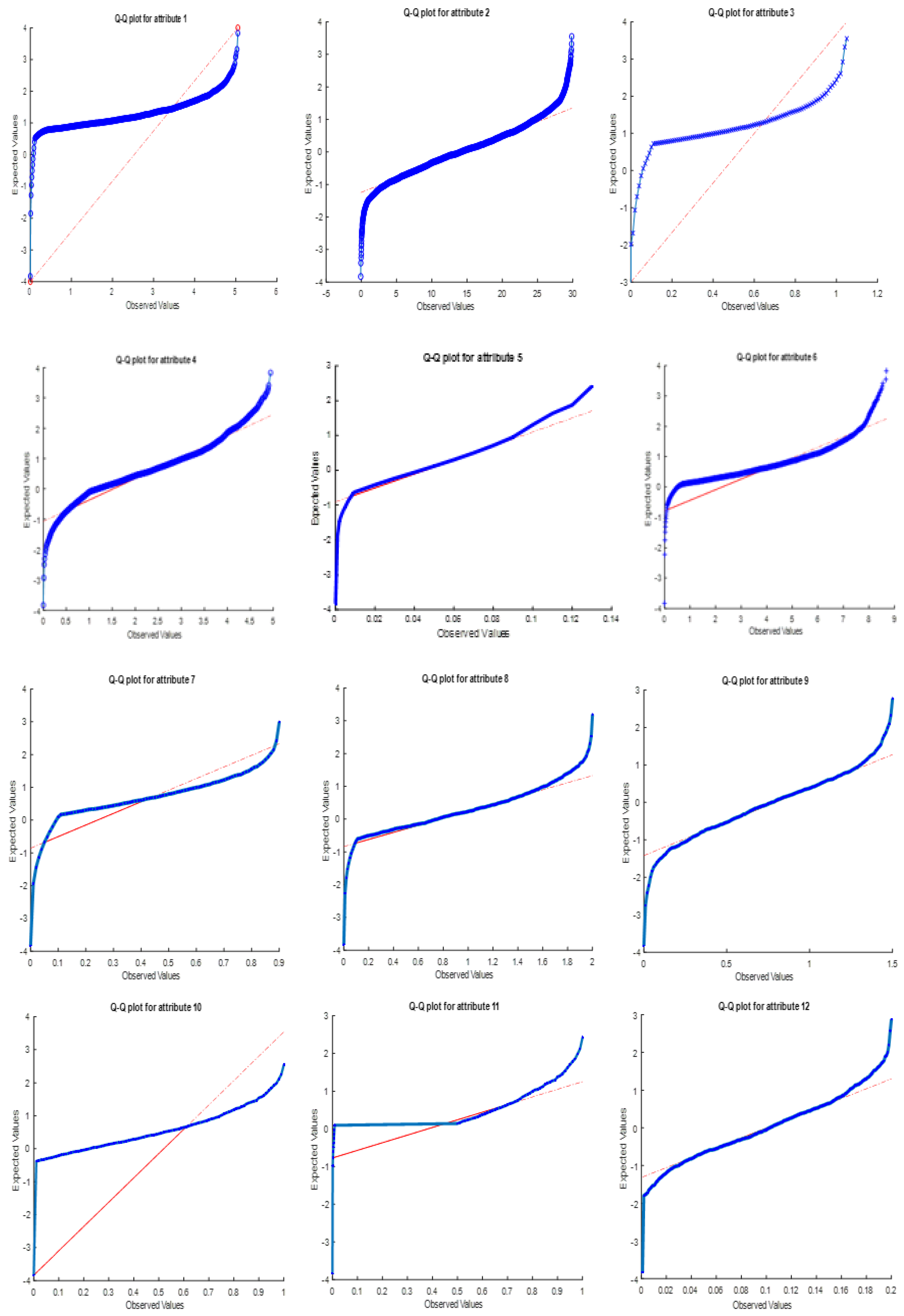
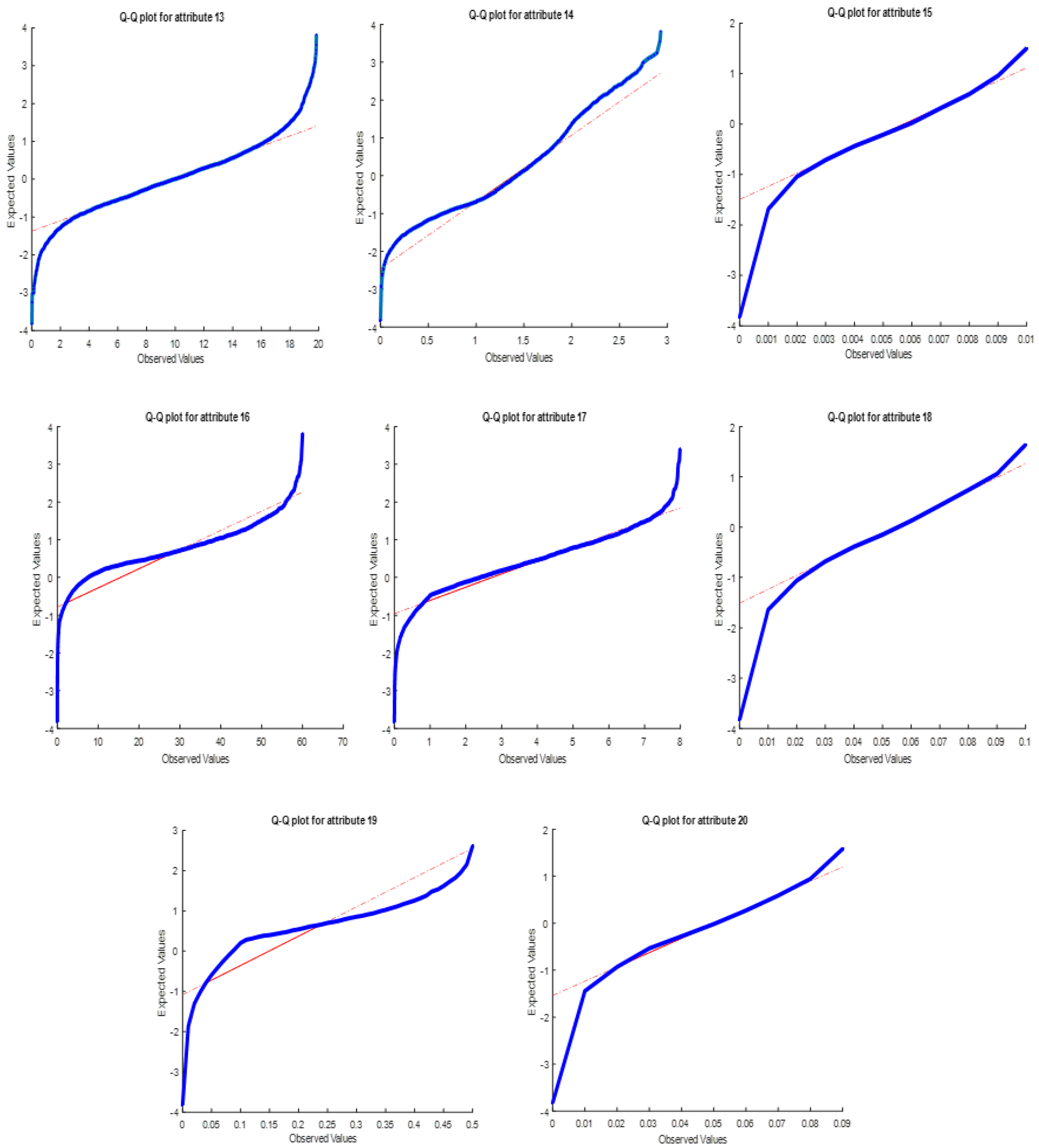
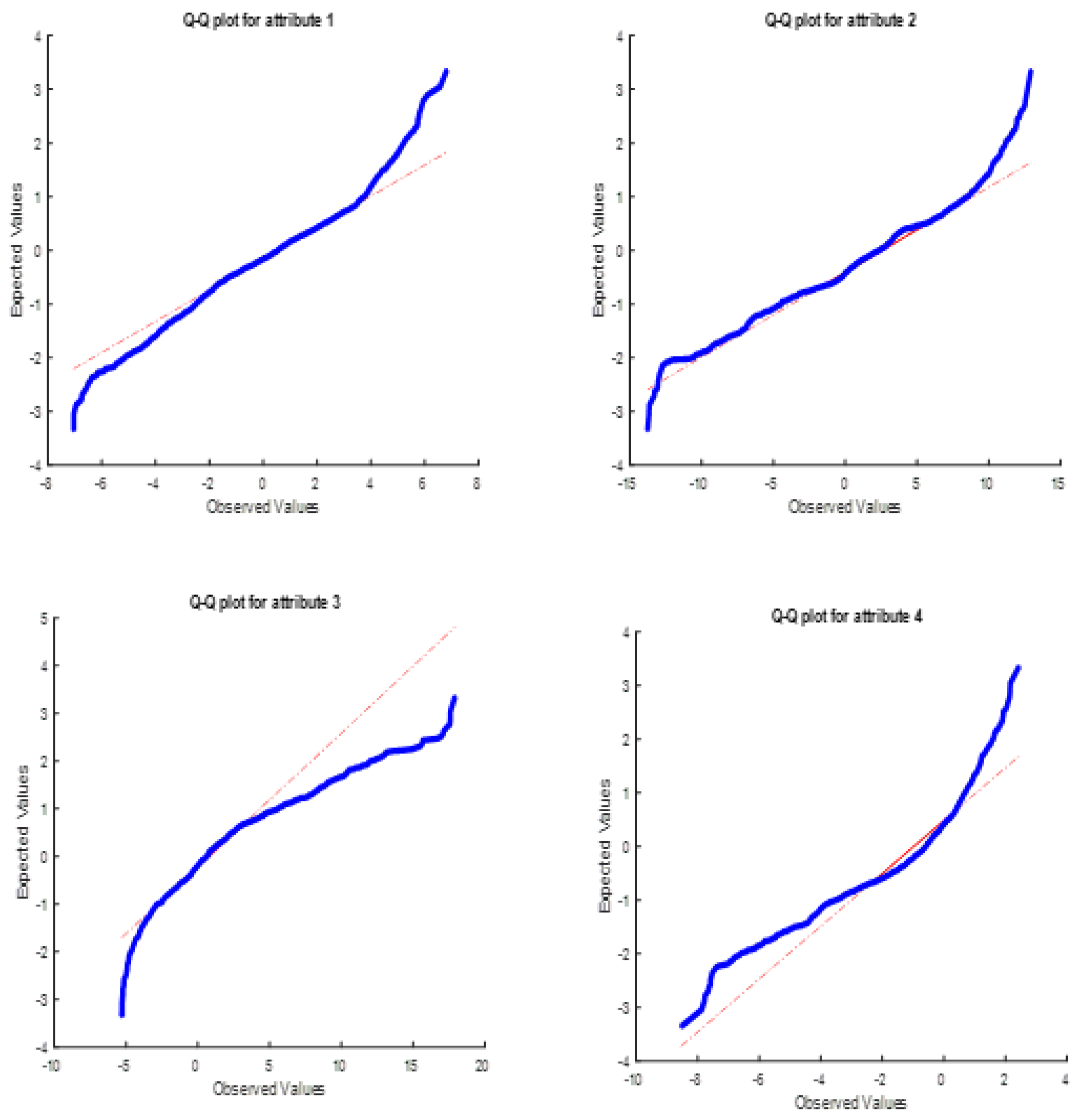
The Q-Q plot graph, which will be drawn using the Z-score values of an attribute in a data set, shows the relationship between the expected distribution values and the actual values. When the relationship between expected and actual values overlaps, a line at a 45-degree angle appears on the graph. Actual values are shown with dots, and the dots are expected to be on or very close to this 45-degree line [
81].
In this part of the study, Q-Q plot graphs of the data sets on which experimental studies were carried out were drawn. In the graphs, it is seen that the clustering accuracies of data sets containing attributes that are distributed outside the normal distribution expected from the attributes are higher. The mathematical meaning of this is this: In distance measure-based clustering approaches, it is the value of the sum of the distances separating the clusters from each other. The more a feature has a distribution different from normal; The effect of the difference value it will create in total will be more significant.
If the data used consists of features close to normal distribution; The effect of all attributes on the total distance will be approximately the same. This will cause the success of clustering to be lower. Q-Q plot graphics of 5 data sets are given in
Figure 15,
Figure 16,
Figure 17,
Figure 18 and
Figure 19.
As can be seen in
Figure 15, the distributions of features 3 and 4 have moved away from the expected 45-degree line in some places. Since the variation in the distribution of these features has a distinctive effect on changing the total distance measure, the success rate in the Iris data set could reach a high value of 95.5%.
As can be seen from
Figure 16, in some parts for attribute 2, but mostly for attributes 3 and 4, the distributions are clearly away from the expected 45-degree line. Since the variation in the distribution of these features has a distinctive effect on changing the total distance measure, the success rate in the OD data set could reach a high value of 95%.
As seen in
Figure 17, since all the features of the WBCO data set have a distribution in regions far from the 45-degree line, this data set was able to reach a success rate of 94%.
As seen in
Figure 18, the WBCO data set has a success rate of 92%, as features 1, 3, 10, 11 are clearly distributed, and features 7, 19 and 20 are distributed in some places far from the 45-degree line. reached its value.
As seen in
Figure 19, all features of the BA data set have a distribution in regions close to the 45-degree slope line. This shows that the distributions of the features are close to the normal distribution. For this reason, it was concluded that the features did not make a sharp distinction in separating the clusters. This data set also had a success rate of 67%.
Clustering methods are divided into two general classes: hierarchical and non-hierarchical. Hierarchical class, agglomerative and divisive; The non-hierarchical class is divided into four subclasses: partitioning, density-based, grid-based, and other approaches [
82]. These methods can greatly affect the success of clustering. In this study, distance measure was used when performing cluster analysis. To increase the success of the data set, the type of cluster analysis can be determined from the beginning. For this reason, the type of cluster analysis can be chosen differently in data sets such as BA, where the Accuracy value is low.
The correlation coefficient between attributes is a criterion that reveals the direction and degree of the relationship between the actual value and the value to be estimated. This coefficient can take values between -1 and 1. If the value is positive, it means that as one of the attributes increases, the other tends to increase as well. When the correlation coefficient is negative, it is understood that while one of the attributes increases, the other tends to decrease. If the correlation coefficient is greater than 0.8, it is a strong correlation between the attributes, and if it is less than 0.5, it is a weak correlation. [
83].
Table 15,
Table 16,
Table 17,
Table 18 and
Table 19 show the correlation matrices showing the correlations of the attributes of the 5 data sets on which experimental studies were conducted. When these tables are evaluated together with
Figure 15,
Figure 16,
Figure 17,
Figure 18 and
Figure 19; It is seen that the correlation values and the Q-Q plot graphics overlap. Therefore, the method in cluster analysis can be determined by considering the status of the data sets. For example, a density-based or grid-based approach can be chosen instead of a distance measure.
Table 15. When examined, it is seen that there is a strong correlation between the attributes of the Iris data set. Only attribute number 2 has a weak negative correlation with the others. This correlation relationship can be seen when looking at the characteristics of the Q-Q plot graphs. The characteristic of the graph and the values of the change intervals are like the characteristic of the other attribute with a strong correlation relationship. Looking at
Figure 15 from this perspective, the strong correlations in
Table 15 manifest themselves in
Figure 15.
When
Figure 16 is examined carefully, it will be seen that the graphic characteristics and change ranges of attributes 2 and 5, which are the strongest correlations in
Table 16, are similar. All attributes of the OD dataset have a positive correlation relationship with another attribute.
As can be seen in
Table 17, there is a strong correlation between the attributes of the WBCO data set. If
Figure 17 is examined carefully, it will be seen that the graphic characteristics and change ranges of features 2 and 3, which are the features with the strongest correlation, are similar
When
Table 18 is examined, it is seen that the graphic characteristics and change intervals of the attributes with the highest correlation are the most similar in
Figure 18.
When
Table 19 is examined, it will be seen that there is no strong positive correlation between the attributes of the BA data set. The clustering success of this data set was lower than the others. If
Figure 19 is examined, the attributes of this data set are close to the 45-degree slope line in the Q-Q plot graph. This shows that the attributes of the data set are insufficient to distinguish the clusters.
7. Conclusions
Meta-heuristic methods are especially preferred in systems that cannot be solved by known classical methods, are difficult to solve, and have many parameters. They have become popular methods widely used in optimization. The fact that there are no restrictions in the field of use makes meta-heuristic methods even more popular.
A new heuristic method is proposed in this study. The Pi Algorithm, inspired by the number Pi, has been successfully applied to clustering. The results are also sufficient in terms of accuracy. Only the success level is low in the BA data set. When looking at the BA data set, it is seen that the correlation between the attributes of the data set is low, and its distribution is far from normal. In future studies, experimental studies of the Pi algorithm can be carried out with different density-based or grid-based methods.
In distance measurements, variables can be greatly affected by the units of measurement. For example, when two solutions are furthest from each other in one unit of measurement; they can become closer to each other when the unit of measurement changes. Therefore, it may be more useful to standardize the features when measuring distance. Feature standardization will also be among the studies that can be done in future experimental studies on the Pi algorithm.
Figure 1.
General meta-heuristic method working principle.
Figure 1.
General meta-heuristic method working principle.
Figure 2.
Representation of numerical integration.
Figure 2.
Representation of numerical integration.
Figure 3.
Application of Monte-Carlo integration.
Figure 3.
Application of Monte-Carlo integration.
Figure 4.
Unit circle application of the Monte-carlo method.
Figure 4.
Unit circle application of the Monte-carlo method.
Figure 5.
Creating random points on the unit circle in the Monte-Carlo method.
Figure 5.
Creating random points on the unit circle in the Monte-Carlo method.
Figure 6.
Graphical representation of clustering.
Figure 6.
Graphical representation of clustering.
Figure 7.
Confusion matrix representation.
Figure 7.
Confusion matrix representation.
Figure 8.
General working principle of the proposed method.
Figure 8.
General working principle of the proposed method.
Figure 9.
Iris dataset confusion matrix results.
Figure 9.
Iris dataset confusion matrix results.
Figure 10.
Confusion matrix results for OD data set.
Figure 10.
Confusion matrix results for OD data set.
Figure 11.
Confusion matrix results for WBCO dataset.
Figure 11.
Confusion matrix results for WBCO dataset.
Figure 12.
Confusion matrix results for WQ dataset.
Figure 12.
Confusion matrix results for WQ dataset.
Figure 13.
Confusion matrix results for the BA dataset.
Figure 13.
Confusion matrix results for the BA dataset.
Figure 14.
Performance result graphs of all data sets.
Figure 14.
Performance result graphs of all data sets.
Figure 15.
Iris data set Q-Q plot.
Figure 15.
Iris data set Q-Q plot.
Figure 16.
OD data set Q-Q plot.
Figure 16.
OD data set Q-Q plot.
Figure 17.
WBCO data set Q-Q plot.
Figure 17.
WBCO data set Q-Q plot.
Figure 18.
WQ data set Q-Q plot.
Figure 18.
WQ data set Q-Q plot.
Figure 19.
BA data set Q-Q plot.
Figure 19.
BA data set Q-Q plot.
Table 1.
An example of a linear relationship.
Table 1.
An example of a linear relationship.
Table 2.
Examples of meta-heuristic methods studied in recent years.
Table 2.
Examples of meta-heuristic methods studied in recent years.
| Algorithm |
Year |
| Pufferfish Optimization Algorithm (POA) [10] |
2024 |
| Elite Opposition-Based Bare Bones Mayfly Algorithm (EOBBMA) [11] |
2024 |
| Literature Research Optimizer (LRO) [12] |
2024 |
| Hippopotamus Optimization Algorithm [13] |
2024 |
| Black-winged kite algorithm (BWKA) [14] |
2024 |
| Drawer Algorithm (DA) [15] |
2023 |
| Special Forces Algorithm (SFA) [16] |
2023 |
| Walrus Optimization Algorithm (WaOA) [17] |
2023 |
| Child Drawing Development Optimization Algorithm (CDDO) [18] |
2022 |
| Equilibrium Slime Mould Algorithm (ESMA) [19] |
2022 |
| Leader Slime Mould Algorithm (LSMA) [20] |
2022 |
| Tuna Swarm Optimization (TSO) [21] |
2021 |
| Dingo Optimization Algorithm (DOA) [22] |
2021 |
| Leader Harris hawks optimization (LHHO) [23] |
2021 |
| Adaptive Opposition Slime Mould Algorithm (AOSMA) [24] |
2021 |
| Hybrid Augmented Grey Wolf Optimizer & Cuckoo Search (AGWOCS) [25] |
2021 |
| Mexican Axolotl Optimization (MAO) [26] |
2021 |
| Golden Eagle Optimizer (GEO) [27] |
2021 |
| Tunicate Swarm Algorithm (TSA) [28] |
2020 |
| Bald eagle search Optimization algorithm (BES) [29] |
2020 |
| Lévy Flight Distribution (LFD) [30] |
2020 |
Table 3.
Pi algorithm best matrix and pi coefficient values for the Iris data set.
Table 3.
Pi algorithm best matrix and pi coefficient values for the Iris data set.
| best |
5.6502 |
3 |
4.2250 |
1.1918 |
| pi |
0.78 |
0.7640 |
0.7880 |
0.8 |
Table 4.
Iris dataset performance results.
Table 4.
Iris dataset performance results.
| |
Accuracy |
Precision |
Recall |
F1 |
| Iris-Setosa |
0,983 |
0,952 |
1 |
0,975 |
| Iris-Versicolor |
0,95 |
0,870 |
1 |
0,93 |
| Iris-Virginica |
0,933 |
1 |
8 |
0,888 |
| Average |
0,955 |
0,941 |
0,933 |
0,931 |
Table 5.
Pi algorithm best matrix and pi coefficient values for OD.
Table 5.
Pi algorithm best matrix and pi coefficient values for OD.
| best |
22.7944 |
34.7413 |
80.0402 |
453.5413 |
0.0056 |
| pi |
0.7920 |
0.7800 |
0.7680 |
0.7240 |
0.8080 |
Table 6.
Performance results for the OD dataset.
Table 6.
Performance results for the OD dataset.
| |
Accuracy |
Precision |
Recall |
F1 |
| Not-occupied |
0,95 |
1 |
0,90 |
0,947 |
| Occupied |
0,95 |
0,909 |
1 |
0,952 |
| Average |
0,95 |
0,955 |
0,95 |
0,950 |
Table 7.
Pi algorithm best matrix and pi coefficient values for WBCO data set.
Table 7.
Pi algorithm best matrix and pi coefficient values for WBCO data set.
| best |
1.9801 |
3.4003 |
1.9869 |
2.8711 |
1.9530 |
| |
3.6583 |
2.5123 |
1.1837 |
3.6278 |
|
| pi |
0.7560 |
0.8280 |
0.7680 |
0.8280 |
0.9080 |
| |
0.8080 |
0.7240 |
0.6880 |
0.7480 |
|
Table 8.
WBCO dataset performance results.
Table 8.
WBCO dataset performance results.
| |
Accuracy |
Precision |
Recall |
F1 |
| Benign |
0,94 |
0,958 |
0,92 |
0,939 |
| Malignant |
0,94 |
0,923 |
0,96 |
0,941 |
| Average |
0,94 |
0,941 |
0,94 |
0,94 |
Table 9.
Pi algorithm best matrix and pi coefficient values for WQ data set.
Table 9.
Pi algorithm best matrix and pi coefficient values for WQ data set.
| |
1.0810 13.3534 0.5427 1.1871 0.0873 2.7346 0.3375 0.6903 0.8522 0.1256 |
| best |
0.4316 0.1424 8.8613 1.4745 0.0066 10.6695 2.7919 0.0316 0.3181 0.0312 |
| Pi |
0.7520 0.7840 0.7320 0.7400 0.8040 0.8200 0.8040 0.7600 0.8400 0.7800 0.8160 0.7400 0.7720 0.7120 0.8000 0.7440 0.8120 0.8160 0.7280 0.8400 |
Table 10.
WBCO dataset performance results.
Table 10.
WBCO dataset performance results.
| |
Accuracy |
Precision |
Recall |
F1 |
| Safe |
0,92 |
0,868 |
0,99 |
0,925 |
| Not safe |
0,92 |
0,988 |
0,85 |
0,914 |
| Average |
0,92 |
0,928 |
0,92 |
0,92 |
Table 11.
Pi algorithm best matrix and pi coefficient values for BA data set.
Table 11.
Pi algorithm best matrix and pi coefficient values for BA data set.
| best |
0.4944 |
2.3023 |
0.6230 |
-0.5922 |
| pi |
0.8360 |
0.7720 |
0.8160 |
0.7200 |
Table 12.
BA dataset performance results.
Table 12.
BA dataset performance results.
| |
Accuracy |
Precision |
Recall |
F1 |
| Genuine |
0,67 |
0,74 |
0,6491 |
0,6916 |
| Forged |
0,67 |
0,6 |
0,6977 |
0,6452 |
| Average |
0,67 |
0,67 |
0,6734 |
0,6684 |
Table 13.
Total performance results for data sets.
Table 13.
Total performance results for data sets.
| |
Accuracy |
Precision |
Recall |
F1 |
| Iris |
0,955 |
0,941 |
0,933 |
0,931 |
| OD |
0,95 |
0,955 |
0,95 |
0,95 |
| WBCO |
0,94 |
0,941 |
0,94 |
0,94 |
| WQ |
0,92 |
0,928 |
0,92 |
0,92 |
| BA |
0,67 |
0,67 |
0,6734 |
0,6684 |
Table 14.
Comparison of the Pi algorithm and some methods in the literature.
Table 14.
Comparison of the Pi algorithm and some methods in the literature.
| Iris Dataset |
|---|
| Author(s) |
Accuracy |
Precision |
Recall |
F1 |
| This study |
0,955 |
0,941 |
0,933 |
0,931 |
| Leela et al. [66] |
0,85 |
- |
- |
- |
| Huang and Gel [67] |
0,78 |
- |
- |
- |
| Gyanaranjan Shial et al. [40] |
0,969 |
- |
- |
0,969 |
| LNC. Prakash K. et al. [41] |
- |
- |
- |
0,82 |
| Occupancy Detection Dataset |
| This study |
0,95 |
0,955 |
0,95 |
0,950 |
| Prabhakaran et al. [68] |
- |
0,783 |
0,621 |
0,845 |
| Fährmann et al. [69] |
0,9590 |
- |
- |
- |
| Huang and Gel [67] |
0,77 |
- |
- |
- |
| Wisconsin Breast Cancer Original Dataset |
| This study |
0,94 |
0,941 |
0,94 |
0,94 |
| Pantazi et al. [70] |
0,953 |
- |
- |
- |
| Dubey et al. [71] |
0,92 |
- |
- |
- |
| Ayoob [72] |
0,965 |
- |
- |
- |
| Lin and Ji [73] |
- |
0,921 |
0,983 |
0,95 |
| Water Quality Dataset |
| This study |
0,92 |
0,928 |
0,92 |
0,92 |
| Eliška Bláhová [74] |
0,855 |
0,791 |
0,973 |
0,873 |
| Banknote Authentication |
| This study |
0,67 |
0,67 |
0,6734 |
0,6684 |
| Guo et al. [45] |
0,8599 |
- |
- |
- |
| Khan M. and Alam M. [75] |
0,87 |
- |
- |
- |
| Alguliyev et al. [76] |
- |
- |
- |
0,6219 |
| Huang and Gel [67] |
0,86 |
- |
- |
- |
| Jadhav and Gomathi [77] |
62,64 |
- |
- |
91,25 |
Table 15.
Iris dataset correlation matrix.
Table 15.
Iris dataset correlation matrix.
| |
1 |
2 |
3 |
4 |
| 1 |
1 |
-0,126 |
0,851 |
0,803 |
| 2 |
-0,126 |
1 |
-0,447 |
-0,357 |
| 3 |
0,851 |
-0,447 |
1 |
0,963 |
| 4 |
0,803 |
-0,357 |
0,963 |
1 |
Table 16.
OD data set correlation matrix.
Table 16.
OD data set correlation matrix.
| |
1 |
2 |
3 |
4 |
5 |
| 1 |
1 |
-0,155 |
0,661 |
0,563 |
0,139 |
| 2 |
-0,155 |
1 |
0,016 |
0,435 |
0,955 |
| 3 |
0,661 |
0,016 |
1 |
0,668 |
0,213 |
| 4 |
0,563 |
0,435 |
0,668 |
1 |
0,627 |
| 5 |
0,139 |
0,955 |
0,213 |
0,627 |
1 |
Table 17.
WBCO data set correlation matrix.
Table 17.
WBCO data set correlation matrix.
| |
1 |
2 |
3 |
4 |
5 |
6 |
7 |
8 |
9 |
| 1 |
1 |
0,656 |
0,667 |
0,510 |
0,537 |
0,633 |
0,584 |
0,556 |
0,361 |
| 2 |
0,656 |
1 |
0,900 |
0,731 |
0,761 |
0,724 |
0,761 |
0,719 |
0,479 |
| 3 |
0,667 |
0,900 |
1 |
0,699 |
0,720 |
0,742 |
0,744 |
0,717 |
0,454 |
| 4 |
0,510 |
0,731 |
0,699 |
1 |
0,615 |
0,687 |
0,664 |
0,607 |
0,448 |
| 5 |
0,537 |
0,761 |
0,720 |
0,615 |
1 |
0,600 |
0,636 |
0,636 |
0,481 |
| 6 |
0,633 |
0,724 |
0,742 |
0,687 |
0,600 |
1 |
0,712 |
0,619 |
0,338 |
| 7 |
0,584 |
0,761 |
0,744 |
0,664 |
0,636 |
0,712 |
1 |
0,674 |
0,381 |
| 8 |
0,556 |
0,719 |
0,717 |
0,607 |
0,636 |
0,619 |
0,674 |
1 |
0,415 |
| 9 |
0,361 |
0,479 |
0,454 |
0,448 |
0,481 |
0,338 |
0,381 |
0,415 |
1 |
Table 18.
WQ data set correlation matrix.
Table 18.
WQ data set correlation matrix.
| |
1 |
2 |
3 |
4 |
5 |
6 |
7 |
8 |
9 |
10 |
11 |
12 |
13 |
14 |
15 |
16 |
17 |
18 |
19 |
20 |
| 1 |
1 |
0,062 |
0,247 |
0,293 |
-0,075 |
0,363 |
0,347 |
0,163 |
-0,010 |
-0,100 |
-0,082 |
0,017 |
-0,007 |
0,235 |
-0,008 |
0,347 |
0,238 |
0,000 |
0,329 |
0,014 |
| 2 |
0,062 |
1 |
0,050 |
0,070 |
-0,001 |
0,105 |
0,122 |
0,015 |
-0,027 |
0,060 |
0,105 |
-0,036 |
0,008 |
-0,067 |
0,021 |
0,086 |
0,049 |
0,030 |
0,075 |
0,015 |
| 3 |
0,247 |
0,050 |
1 |
0,371 |
0,329 |
0,368 |
0,324 |
-0,035 |
0,004 |
0,040 |
0,011 |
-0,089 |
0,028 |
0,308 |
-0,016 |
0,352 |
0,226 |
-0,009 |
0,319 |
0,001 |
| 4 |
0,293 |
0,070 |
0,371 |
1 |
-0,030 |
0,451 |
0,420 |
0,062 |
-0,018 |
0,095 |
-0,008 |
-0,047 |
-0,015 |
0,311 |
0,001 |
0,464 |
0,288 |
0,033 |
0,434 |
-0,004 |
| 5 |
-0,075 |
-0,001 |
0,329 |
-0,030 |
1 |
-0,133 |
-0,147 |
-0,104 |
0,004 |
-0,083 |
0,026 |
-0,035 |
0,025 |
-0,010 |
-0,016 |
-0,129 |
-0,090 |
0,010 |
-0,145 |
-0,005 |
| 6 |
0,363 |
0,105 |
0,368 |
0,451 |
-0,133 |
1 |
0,559 |
0,113 |
0,006 |
0,146 |
-0,003 |
-0,034 |
-0,008 |
0,378 |
-0,023 |
0,591 |
0,389 |
0,013 |
0,525 |
-0,006 |
| 7 |
0,347 |
0,122 |
0,324 |
0,420 |
-0,147 |
0,559 |
1 |
0,108 |
-0,002 |
0,133 |
-0,005 |
-0,053 |
-0,017 |
0,336 |
-0,023 |
0,527 |
0,318 |
0,033 |
0,514 |
-0,007 |
| 8 |
0,163 |
0,015 |
-0,035 |
0,062 |
-0,104 |
0,113 |
0,108 |
1 |
0,012 |
0,147 |
0,003 |
0,121 |
-0,001 |
0,159 |
0,014 |
0,097 |
0,023 |
-0,007 |
0,083 |
0,006 |
| 9 |
-0,010 |
-0,027 |
0,004 |
-0,018 |
0,004 |
0,006 |
-0,002 |
0,012 |
1 |
0,016 |
0,020 |
0,014 |
-0,009 |
-0,015 |
-0,005 |
-0,017 |
0,009 |
0,023 |
0,014 |
0,015 |
| 10 |
-0,100 |
0,060 |
0,040 |
0,095 |
-0,083 |
0,146 |
0,133 |
0,147 |
0,016 |
1 |
0,612 |
-0,031 |
-0,040 |
0,240 |
-0,006 |
0,135 |
0,092 |
-0,006 |
0,139 |
0,042 |
| 11 |
-0,082 |
0,105 |
0,011 |
-0,008 |
0,026 |
-0,003 |
-0,005 |
0,003 |
0,020 |
0,612 |
1 |
0,015 |
-0,049 |
-0,103 |
0,012 |
-0,005 |
-0,026 |
-0,036 |
0,004 |
0,055 |
| 12 |
0,017 |
-0,036 |
-0,089 |
-0,047 |
-0,035 |
-0,034 |
-0,053 |
0,121 |
0,014 |
-0,031 |
0,015 |
1 |
0,033 |
-0,058 |
-0,007 |
-0,031 |
-0,053 |
0,031 |
-0,063 |
-0,011 |
| 13 |
-0,007 |
0,008 |
0,028 |
-0,015 |
0,025 |
-0,008 |
-0,017 |
-0,001 |
-0,009 |
-0,040 |
-0,049 |
0,033 |
1 |
0,011 |
-0,021 |
-0,022 |
-0,025 |
0,041 |
0,001 |
-0,001 |
| 14 |
0,235 |
-0,067 |
0,308 |
0,311 |
-0,010 |
0,378 |
0,336 |
0,159 |
-0,015 |
0,240 |
-0,103 |
-0,058 |
0,011 |
1 |
-0,020 |
0,344 |
0,271 |
0,010 |
0,331 |
-0,012 |
| 15 |
-0,008 |
0,021 |
-0,016 |
0,001 |
-0,016 |
-0,023 |
-0,023 |
0,014 |
-0,005 |
-0,006 |
0,012 |
-0,007 |
-0,021 |
-0,020 |
1 |
0,003 |
0,031 |
0,034 |
0,004 |
0,033 |
| 16 |
0,347 |
0,086 |
0,352 |
0,464 |
-0,129 |
0,591 |
0,527 |
0,097 |
-0,017 |
0,135 |
-0,005 |
-0,031 |
-0,022 |
0,344 |
0,003 |
1 |
0,370 |
0,014 |
0,503 |
-0,001 |
| 17 |
0,238 |
0,049 |
0,226 |
0,288 |
-0,090 |
0,389 |
0,318 |
0,023 |
0,009 |
0,092 |
-0,026 |
-0,053 |
-0,025 |
0,271 |
0,031 |
0,370 |
1 |
0,030 |
0,352 |
0,019 |
| 18 |
0,000 |
0,030 |
-0,009 |
0,033 |
0,010 |
0,013 |
0,033 |
-0,007 |
0,023 |
-0,006 |
-0,036 |
0,031 |
0,041 |
0,010 |
0,034 |
0,014 |
0,030 |
1 |
-0,020 |
-0,025 |
| 19 |
0,329 |
0,075 |
0,319 |
0,434 |
-0,145 |
0,525 |
0,514 |
0,083 |
0,014 |
0,139 |
0,004 |
-0,063 |
0,001 |
0,331 |
0,004 |
0,503 |
0,352 |
-0,020 |
1 |
0,008 |
| 20 |
0,014 |
0,015 |
0,001 |
-0,004 |
-0,005 |
-0,006 |
-0,007 |
0,006 |
0,015 |
0,042 |
0,055 |
-0,011 |
-0,001 |
-0,012 |
0,033 |
-0,001 |
0,019 |
-0,025 |
0,008 |
1 |
Table 19.
BA data set correlation matrix.
Table 19.
BA data set correlation matrix.
| |
1 |
2 |
3 |
4 |
| 1 |
1,000 |
0,265 |
-0,377 |
0,275 |
| 2 |
0,265 |
1,000 |
-0,789 |
-0,524 |
| 3 |
-0,377 |
-0,789 |
1,000 |
0,322 |
| 4 |
0,275 |
-0,524 |
0,322 |
1,000 |
