Preprint
Article

Dynamics of SEPAIVRD model for COVID-19 in Bangladesh

Altmetrics

Downloads

71

Views

41

Comments

0

This version is not peer-reviewed

Submitted:

05 September 2024

Posted:

06 September 2024

You are already at the latest version

Alerts
Abstract
Background: Since 2020, when the Covid-19 outbreak began, researchers worldwide have been investigating its biological processes, transmission patterns, and the mathematical expression of this infectious disease. Multiple mathematical models have been presented thus far, with the simplest being the SIR model. The question now is whether the SIR model can provide a comprehensive representation of Covid-19 or if a more intricate model is necessary. With this in mind, the SEPAIVRD model has been developed. Objective: This study focuses on understanding the third wave of Covid-19 that began in mid-May 2021 in Bangladesh. To achieve this, we introduced three essential compartments in our model: Presymptomatic (P), Asymptomatic (A), and Vaccinated (V) classes. The Asymptomatic class will help us determine how close the population is to achieving herd immunity. The Presymptomatic class will provide insight into whether we can effectively control Covid-19 by identifying infected individuals over an extended period. Lastly, the Vaccinated class will allow us to explore how the Presymptomatic class affects those who have received the vaccine. The results of this study aim to address these questions. Findings: According to the study findings, an increase in vaccination rates could result in a decrease in the number of people getting infected every day, lessening the strain on healthcare resources and lowering the risk of transmission to others. Moreover, the research highlights the significance of using highly effective vaccines to combat COVID-19 cases and fatalities, particularly in areas with low vaccination rates. Additionally, implementing social distancing measures can be an effective approach to contain the spread of the virus by reducing the effective contact rate. Conclusion: The model presented in this study provides a comprehensive overview of Covid-19 transmission in Bangladesh. Furthermore, this model can be applied to other countries in South Asia and is therefore a valuable mathematical model for understanding Covid-19.
Keywords: 
Subject: Computer Science and Mathematics  -   Mathematical and Computational Biology

1. Introduction

The Covid-19 pandemic, caused by the novel coronavirus SARS-CoV-2, has brought significant changes to the world in the past few years. The virus first emerged in Wuhan, China, in late 2019 and has since spread rapidly worldwide, resulting in numerous deaths and overwhelming healthcare systems. Covid-19 is primarily transmitted through respiratory droplets, and its symptoms can range from mild flu-like symptoms to severe respiratory illness, leading to hospitalization and death. Governments worldwide have implemented various measures to curb the spread of Covid-19, including social distancing, face mask mandates, and vaccination campaigns. Despite these efforts, Covid-19 remains a significant global health challenge, with new variants emerging and the virus continuing to spread. Understanding the virus's transmission dynamics and developing effective prevention and treatment strategies are critical in managing the ongoing Covid-19 pandemic.
According to Barlow & Weinstein's [1] research, they employed asymptotic approximations to develop a closed-form analytical solution of the SIR model and utilized this solution to describe the characteristics of COVID-19. By comparing the SIR model approximations with real-time COVID-19 data from Japan, they established a strong correlation between the two. Tomchin & Fradkov [2] focused on predicting the behavior of COVID-19 in Russia using discrete-time SIR and SEIR models. Initially, they utilized a discrete-time SIR model that excluded the asymptomatic class. However, they later improved their model by incorporating asymptomatic individuals in the exposed class and presented a discrete-time SEIR model. Through the application of the inverse method, Marinov & Marinova [3] investigated the dynamics of the SIR model across 12 different countries by comparing and analyzing real-time data. While acknowledging the constraints of the epidemic model, they made short-term predictions regarding the progression of the disease. Neves & Guerrero [4] focused on forecasting the potential outcomes of COVID-19 endemics in Lombardy, Italy, and Sao Paulo, Brazil. To achieve this, they employed the SAIR model, which includes an asymptomatic class.
The work of Alenezi et al. [5] involved the development of SIR and SEIR models to approximate the COVID-19 outbreak in Kuwait. They discovered that the basic reproduction number varied from 3 to 4, indicating that the failure to implement effective measures to curb the spread of COVID-19 would result in exponential growth of cases. Din & Algehyne [6] presented a novel version of the SIR model and evaluated its performance by comparing it with real COVID-19 data from Pakistan. In contrast, Malavika et al. [7] utilized the SIR model with a logistic growth curve to make short-term predictions regarding COVID-19 behavior in India. According to their study, lockdown measures may not have a significant impact on reducing the infection rate. Kozyreff [8] expanded on the SIR model by including individuals infected with COVID-19 who require hospitalization. They evaluated their findings by comparing them to real-world data from various countries, and concluded that models with curved fitting achieved higher accuracy. Conversely, Campos et al. [9] developed a discrete-time SIR model to predict the age-based vaccination strategy for COVID-19 in Brazil. Their research indicated that vaccinating different age groups could significantly reduce the number of deaths caused by the virus. Kudryashov et al. [10] utilized an analytical approach to explore the potential application of the SIR model in predicting the behavior of COVID-19. They suggested that while the SIR model may be useful for short-term predictions and small populations, modifications are required to make accurate long-term forecasts. Nonetheless, the model's simplicity has contributed to its widespread use in research for several decades. Researchers such as Cooper et al. [11], Nesteruk [12,13], Turkyilmazoglu [14], Anand et al. [15], and Lounis and Bagal [16] have also used the SIR model in various studies related to COVID-19.
Ramos et al. [17] developed the θ-SEIHQRD model to better understand the COVID-19 outbreak in Italy. In their model, they extended the classical Susceptible-Infectious-Recovered (SIR) model to include additional compartments such as Exposed (E), Hospitals (H), Quarantine (Q), and Deaths (D). By incorporating these compartments, they were able to obtain a more accurate representation of the real situation of COVID-19 in Italy. Their findings showed good agreement with the real-world data, and they also provided insights on potential future observations. Shahrear et al. [18] developed a mathematical model called the SEQIRP model to forecast the spread of COVID-19 in Bangladesh. They solved the system of first-order nonlinear ordinary differential equations with the given initial conditions using the Runge-Kutta method of order four. Their numerical investigation showed that temperature plays a significant role in the transmission of COVID-19, and that other countries have also faced similar issues. Uddin et al. [19] suggested that the winter season may not be favorable for people in Bangladesh as low temperatures could contribute to the rapid spread of COVID-19. However, Ahmed et al. [20] recently discussed that temperature and humidity have very little impact on the fast transmission of COVID-19. They argued that high population density, poor air quality, and inadequate COVID-19 testing have a more significant effect on the increase of COVID-19 cases.
The COVID-19 situation in Malaysia and Pakistan was studied by Alrabaiah et al. [21] using the fractional-order SEIQRDC model, which included a compartment for the protected population class called C. They attributed the rapid spread of COVID-19 in Pakistan to factors such as high population density, poor economic conditions, and inadequate safety measures. This finding is consistent with the research outcomes of Ahmed et al. [20]. A modified SEIR model was presented by López & Rodó [22] to forecast the spread of COVID-19 in Italy and Spain. Their model included a confined susceptible class, quarantine class, and dead population class. The modified model displayed stable behavior and was able to forecast future outcomes. Meanwhile, Hussain et al. [23] utilized the SEIQR model to conduct an analytical study and predict the future situation of COVID-19 in Pakistan. A SEIAR model was proposed by Li et al. [24] to highlight the importance of human awareness and social distancing in mitigating the spread of COVID-19. On the other hand, Youssef et al. [25] examined the spread of COVID-19 in Saudi Arabia using the SEIQR model. They conducted an analysis of reproduction numbers, equilibrium points, and stability, and utilized the Lyapunov stability theorem to demonstrate global stability. Their model was validated using actual COVID-19 data, and they found it to be in good agreement. Yu et al. [26] proposed a delay-SEIRS model to analyze the COVID-19 pandemic. They argued that social distancing, quarantine, and lockdown measures may not significantly reduce the transmission of COVID-19, but could have a substantial negative impact on the global economy. In addition to their work, Adhikary & Pal [27], Akindeinde et al. [28], Basnarkov [29], Khedher et al. [30], Pekpe et al. [31], Zhu & Shen [32], Chen et al. [33], Contreras et al. [34], and León et al. [35] have also studied modified and extended SIR models to investigate COVID-19.
To accurately portray the COVID-19 situation in Bangladesh through our research, we must construct a fresh model and ensure that it adheres to certain guidelines:
Step 1: Our research requires us to validate the compartments and ensure that each class holds significant implications for presenting accurate scenarios. For instance, the presymptomatic class holds immense significance since a large number of individuals in Bangladesh fail to comply with COVID-19 guidelines until they test positive. This is a key reason why the presymptomatic class tends to infect densely populated areas more easily. Additionally, lockdown measures are not very effective in Bangladesh since individuals with low income need to venture outside in search of work to sustain themselves. Due to a disregard for health regulations, a large number of individuals in the vulnerable class frequently venture outdoors. It is presumed that many of these individuals have obtained herd immunity against COVID-19, and consequently, do not undergo testing since they exhibit no symptoms. A recent study conducted by icddr,b, and Bangladesh Health Watch revealed that approximately 72% of low-income residents in Dhaka and Chattogram have developed antibodies. Some of these individuals experienced mild symptoms, while the majority remained asymptomatic. Hence, this particular segment of the population is categorized as the asymptomatic class. It should also be noted that the vaccinated class has emerged recently, following the Bangladesh government's decision to provide free vaccines to the public from February 7, 2021, onwards. Despite being vaccinated, individuals within this group remain susceptible to contracting COVID-19.
Step 2: The time has come to deliberate on the model's parameters. To proceed with caution, we will adopt a three-pronged approach. Firstly, we will gather data from various sources. Secondly, we will derive some parameter values from real-world data. Thirdly, we will make certain assumptions. Once we have estimated the parameter values, we can conduct simulations and compare the results with actual data. Furthermore, we will verify the precision of the present code by cross-checking it against other researchers' findings.
Step 3: Our objective is to forecast the future outcomes of the COVID-19 situation in Bangladesh and also illustrate the potential future scenarios of other South Asian countries.

2. Mathematical Modelling

Let us define each compartment of the model:
S: The susceptible class comprises individuals who have either never been infected by COVID-19 or have fully recovered from the virus.
E: The exposed class consists of individuals who are at risk of being infected by COVID-19.
P: The presymptomatic class includes individuals who have been infected with COVID-19 but have yet to display any symptoms. These individuals will eventually develop symptoms and can transmit the virus to others during this asymptomatic period. They may wait for symptoms to appear before getting tested and, in the interim, unwittingly spread COVID-19 within their local communities. Once they receive a positive COVID-19 test result, they are moved to the infected class.
A: The asymptomatic class comprises individuals who have been infected with COVID-19 but do not display any symptoms. Despite being asymptomatic, they can still transmit the virus to others. At times, the asymptomatic class is also referred to as the mild-symptomatic class, where individuals exhibit symptoms similar to seasonal flu and recover naturally without requiring any treatment. As a result, they may not opt for COVID-19 testing and remain within the asymptomatic class. This class can offer insights into the development of herd immunity against COVID-19. It's worth noting that individuals in the asymptomatic class are not considered part of the infected class.
I: The infected class consists of individuals who have been infected with COVID-19 and received a positive test result. These individuals may receive treatment either in hospitals or at home.
V: The vaccinated class refers to individuals who have received one or two doses of COVID-19 vaccines and have either fully recovered from COVID-19 or have never been infected before. While they have some protection against COVID-19, there is still a possibility of getting infected between doses or even after completing the vaccination regimen, depending on the COVID-19 variants. Therefore, individuals in this class should strictly adhere to all health protocols and precautions as they still have a chance of contracting the virus.
R: The Recovered class comprises people who have fully recovered from COVID-19 and moved to the susceptible class. These individuals have successfully gone through the infected and quarantine stages, overcome the severity of COVID-19, and received post-treatment care, resulting in their recovery from the virus and the development of immunity. After being exposed to COVID-19, this class of people generates antibodies within a few days or weeks.
D: The Death class refers to the group of people who have passed away solely due to COVID-19 infection.
In this paper, we have considered a deterministic system of non-linear differential equations to formulate the model. The total human population, Nh (t), is divided into the following eight compartments: susceptible individuals (S), vaccinated individuals (V), individuals exposed with COVID-19 (E), pre-symptomatic individuals (P), asymptomatic individuals (A), COVID-19 infected individuals (I), recovered individuals (R).
λ = β I + τ P
Assuming a constant recruitment rate (Λ) during the model formulation, the rate of susceptible individuals getting infected with COVID-19 is denoted by λ . Another assumption is that individuals who have recovered from COVID-19 may become susceptible again. Based on these assumptions, we can derive the following set of differential equations.
d S d t = Λ β I + τ P S + σ R K 1 S
d V d t = ρ S 1 ε β I + τ P V K 2 V
d E d t = β I + τ P S + 1 ε β I + τ P V K 3 E
d P d t = ω E K 4 P
d A d t = ω E K 5 A
d I d t = ω E + κ 1 P K 6 I
d R d t = κ 2 I K 7 R
d D d t = γ I
where
K 1 = ρ + μ ,   K 2 = μ ,   K 3 = 3 ω + μ ,   K 4 = κ 1 I + μ ,   K 5 = μ ,   K 6 = γ I + κ 2 + μ ,   K 7 = σ + μ .
Here β is the rate of contact for COVID-19 infection. The modification parameters τ < 1 indicate low infectiousness of the individuals in the P class compared to the individuals in the I class. ρ is the vaccination rate provided to susceptible individuals. Susceptible populations move to the exposed class at a rate λ upon contact with infected individuals. Due to immunity, among the susceptible individuals those who are vaccinated moved to the exposed class at a lower rate ( 1 ε )   λ . Individuals exposed to COVID-19 progress to the P, A and I classes at a rate ω . Individuals in the pre-symptomatic class (P) move to the infected class (I) at a rate κ 1 . κ 2 represents the recovery rate of infected individuals. γ is the disease-induced death rate for infected individuals in I class. µ corresponds to the natural death rate. Recovered individuals move to the susceptible class at a rate σ .
Initial Conditions:
S 0 = S 0 ,   E 0 = E 0   P 0 = P 0 ,   A 0 = A 0 ,   I 0 = I 0 , V 0 = V 0 ,   R 0 = R 0 ,   D 0 = D 0

3. Mathematical analysis of the COVID-19 model

3.1. Positivity and Boundedness of the Solution of the Model

We have the following theorem.
Theorem 1: If S ( 0 ) 0 ,   V ( 0 ) 0 ,   E ( 0 ) 0 ,   P ( 0 ) 0 ,   A ( 0 ) 0 ,   I ( 0 ) 0   a n d   R ( 0 ) 0 and all the parameters are positive then solutions S ,   V ,   E c ,   I c ,   H   a n d   R of the system (2) will remain positive and bounded for all time t > 0 .
Proof. From the first equation of model (2) we
d d t S t exp   0 t λ r d r + K 1 t Λ exp   0 t λ r d r + K 1 t
Solving the differential equation (3), the following expression can be obtained
S t exp   0 t λ r d r + K 1 t S 0 0 t Λ exp   0 x λ r d r + K 1 t d x
which can also be written as,
S t S 0 exp   0 t λ r d r + K 1 t + exp   0 t λ r d r + K 1 t 0 t Λ exp   0 x λ r d r + K 1 t d x > 0
Similar expressions can be found for other variables and hence, we have
V 0 ,   E 0 ,   P 0 ,   A 0 ,   I 0 ,   a n d   R 0 for all t 0 .
Now adding all the equations of model (2), we can obtain
d N d t = Λ μ N γ I
Again, we can write
Λ μ + γ N h d N d t Λ μ N
Hence,
Λ μ + δ 1 lim t   inf   N lim t   sup   N Λ μ
which implies
lim t   sup   N Λ μ
Again equations (4) and (5) implies
d N d t Λ μ N
N t N 0 e μ t + Λ μ 1 e μ t
When
t = 0 ,   N t Λ μ   i f   N 0 Λ μ
implying the region = ( S ,   V ,   E ,   P ,   A ,   I ,   R )   ϵ R + 7 :   N Λ μ is positively invariant [39]. Hence all the solutions of model (2) remains in for all time t > 0 .

1.2. Local Asymptotic Stability of the DFE

From the COVID-19 model (2), the disease-free equilibrium (DFE), D , is obtained as
D = S * ,   V * ,   E * ,   P * ,   A * ,   I * ,   R * = ( Λ ρ + μ ,   Λ ρ μ ρ + μ ,   0 ,   0 ,   0 ,   0 ,   0 )
The local asymptotic stability of the DFE can be established using the next-generation operator method [36,37] on the system (2). For system (2), we have
F = 0 τ F 0 F 0 0 0 0 0 0 0 0 0 0 0 0 ,   V = K 3 0 0 0 ω K 4 0 0 ω ω 0 κ 1 K 5 0 0 K 6
where, F associates with new infection terms and V represents the remaining transfer terms and
F = β S + 1 ε V .
Following the approach described in Chavez et al. [38] and Hethcote [39], it can be shown that the control reproduction number, denoted by R c , is given by
R c = τ F ω K 3 K 4 + F ω K 4 μ K 3 K 5
Using Theorem 2 of Van den Driessche and Watmough [37] the following result can be established.
Lemma 1. The DFE of the COVID-19 model (2), is locally-asymptotically stable (LAS) if R c < 1 and unstable if R c > 1 .

3.3. Endemic Equilibrium Point (EEP)

Let E c = S * , V * , E * , P * , A * , I * , R * be any arbitrary equilibrium of the model (2) and let
λ * = β I * + τ P *
be the force of infection at steady-state. Now, setting the left-hand side of each equation of the model (2), the following expressions can be obtained:
S * = Λ + σ R * λ * + K 1 ,   V * = ρ S * 1 ε λ * + K 2 ,   E * = λ * a 1 λ * + a 2 a 3 λ * 2 + a 4 λ * + a 5 , P * = a p   E * ,   A * = a a   E * ,   I * = a i   E * ,   R * = a r   E *
where
a 1 = Λ 1 ε ,   a 2 = Λ 1 ε ρ + K 2 ,   a 3 = 1 ε K 3 ,   a 4 = K 3 K 2 + 1 ε K 1 a 5 = K 1 K 2 K 3 ,   a P = 2 ω K 4 K 1 ,   a a = ω K 5 ,   a i = ω + κ 1 a P K 6 ,   a r = κ 2 K 7 a i
Substituting (10) into (9) gives
λ * = β a i   + τ a p λ * a 1 λ * + a 2 a 3 λ * 2 + a 4 λ * + a 5
After some algebraic calculation the following polynomial equation can be obtained in terms of λ * :
λ * P 2 λ * 2 + P 1 λ * + P 0 = 0
where
P 2 = a 3
P 1 = a 4 β a i + τ a p a 1
P 0 = a 5 β a i + τ a p a 2
Out of the three roots, the root λ * = 0 , of Eq. (12), corresponds to the DFE ( D ) . Equation (12) says that the non-zero equilibria of the model satisfy
f λ * = P 2 λ * 2 + P 1 λ * + P 0 = 0
We have the following result.
Theorem 2. The COVID-19 only model (2) has
(a) A unique endemic equilibrium if P 0 < 0 (i.e.  R c > 1 ),
(b) A unique endemic equilibrium if P 1 < 0   a n d   P 0 = 0   o r   P 1 2 4 P 2 P 0 = 0 ,
(c) Two endemic equilibria if P 1 < 0   a n d   P 0 > 0 i . e . R c < 1   a n d   P 1 2 4 P 2 P 0 > 0
(d) No endemic equilibrium otherwise.

3.4. Backward Bifurcation Analysis of the COVID-19 Model
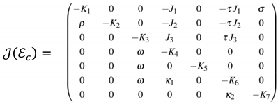
From condition-(c) of Theorem 2, we have the possibility of having two endemic equilibrium whenever R c < 1 and hence there may exist backward bifurcation phenomenon. Now we will apply center manifold theory [37,40] to examine the existence of backward bifurcation. For this let us consider the changes of variable as S = x 1   ,   V = x 2 ,   E = x 3 ,   P = x 4 ,   A = x 5 ,   I = x 6 ,   a n d   R = x 7 , so that in vector form the model (2) can be written as
d X d t = f 1 , f 2 , f 3 , f 4 , f 5 , f 6 , f 7 T
where X = ( x 1 , x 2 , x 3 , x 4 , x 5 , x 6 , x 7 ) T and then we have
d x 1 d t = f 1 = Λ β x 6 + τ x 4 x 1 + σ x 7 K 1 x 1
d x 2 d t = f 2 = ρ x 1 1 ε β x 6 + τ x 4 x 2 K 2 x 2
d x 3 d t = f 3 = β x 6 + τ x 4 x 1 + 1 ε β x 6 + τ x 4 x 2 K 3 x 3
d x 4 d t = f 4 = ω x 3 K 4 x 4
d x 5 d t = f 5 = ω x 3 K 5 x 5
d x 6 d t = f 6 = ω x 3 + κ 1 x 4 K 6 x 6
d x 7 d t = f 7 = κ 2 x 6 K 7 x 7
The Jacobian of the system (14) is given by:
Preprints 117386 i001
where
J 1 = β Λ ρ + μ ,   J 2 = 1 ε ρ β Λ μ ρ + μ ,   J 3 = β 1 ε ρ + μ Λ μ ρ + μ
Now consider, R c = 1   a n d   β = β * is a bifurcation parameter. Thus we get,
β = β * = μ   K 3 K 4 K 5 τ ω μ K 5 + ω K 4 2 S * + 1 ε V *
The Jacobian J E c of (14) with β = β * , denoted by J β * , has a simple zero eigenvalue (with all other eigenvalues having negative real part). Hence, the center manifold theory can be used to analyze the dynamics of the model (2).
Eigenvector of J β * = J E c β = β * :
When R c = 1 , the Jacobian ( J β * ) of (14) has a right eigenvector given by W = ( w 1 , w 2 , w 3 ,   w 4 , w 5 ,   w 6 , w 7 ) T where,
w 1 = J 1 w 4 + τ J 1 w 6 σ w 7 K 1 ,   w 2 = ρ w 1 J 2 w 4 + τ J 2 w 6 K 2 ,   w 3 = w 3 ,
w 4 = ω   w 3 K 4 ,   w 5 = ω   w 3 K 5 ,   w 6 = ω   w 3 + κ 1 w 4 K 6 ,   w 7 = κ 2 w 6 K 7
Further, J β * has a left eigenvector v = [ v 1 , v 2 , v 3 , v 4 , v 5 , v 6 , v 7 ] , where,
v 1 = v 2 = 0 ,   v 3 = ω v 4 + v 6 K 3 , v 4 = v 4 ,   v 5 = 0 ,   v 6 = v 6 ,   v 7 = 0
Computation of a and b [40,41]:
After some tedious manipulations it can be shown that
a = 2   v 3   β τ w 6 + w 4 w 1 + w 2 1 ε
b = Λ v 3 τ w 6 + w 4 μ + ρ 1 ε μ μ + ρ
Thus, it follows from Theorem 4.1 of Castillo-Chavez & Song [41] that the COVID-19 model (2) undergoes backward bifurcation at R c = 1 whenever a > 0   a n d   b > 0 .

3.4.1. Local asymptotic stability of Endemic Equilibrium Point (EEP) for the COVID-19 model

Theorem 3. The EEP of the COVID-19 model (2) given by E c , is locally asymptotically stable (LAS) whenever R c > 1 .

3.5. Global Stability of DFE When There Is No Re-Infection

Theorem 4. The DFE of the COVID-19 model (2) with no re-infection, given by D , is globally asymptotically stable (GAS) whenever R c 1 .
Proof. We consider the following linear Lyapunov function:
L = l v 1 E + l v 2 E + l v 3 I ,
where,
l v 1 = τ ω K 3 K 4 + ω K 3 K 5 + ω κ 1 K 3 K 4 K 5 ,   l v 2 = τ K 4 + κ 1 K 4 K 5 ,   l v 3 = 1 K 5
Differentiating the above Lyapunov function and substituting the expression of E ˙ , P ˙ ,   a n d   I ˙ , we have the following
L ˙ τ P R c 1
Also L ˙ = 0 if and only if R c = 1 . Hence L ˙ 0 . Therefore, L is a Lyapunov function on D and thus it follows by the LaSalle’s invariance principle [42] that, the DFE of the model (2) is globally asymptotic stable whenever R c 1 .

3.6. R c Sensitivity Analysis

In order to manage the disease, it is necessary to ensure that R c is less than 1. This can be achieved by regulating the model parameters that influence the value of R c . If the differentiation of R c with respect to a specific parameter yields a positive sign, it means that increasing (decreasing) the parameter value will cause R c to increase (decrease). Conversely, if the differentiation of R c with respect to a parameter yields a negative sign, it implies that decreasing (increasing) the parameter value will lead to an increase (decrease) in R c . It can be easily verified that
R c τ = β   Λ μ + ρ ε ρ ω μ μ + ρ μ + 3 ω μ + κ 1 > 0 R c ω = β   Λ μ + ρ ε ρ μ τ γ + 2 μ κ 1 + κ 1 2 + μ μ + μ τ + τ κ 2 μ μ + ρ μ + 3 ω 2 μ + κ 1 μ + γ + κ 2 > 0 R c ρ = β   Λ ω ε μ τ γ + 2 μ κ 1 + κ 1 2 + μ μ + μ τ + τ κ 2 μ μ + ρ 2 μ + 3 ω 2 μ + κ 1 μ + γ + κ 2 < 0 R c γ = β   Λ μ + ρ ε ρ μ + κ 1 μ 2 μ + ρ μ + 3 ω μ + γ + κ 2 2 < 0 R c κ 2 = β   Λ μ + ρ ε ρ μ + κ 1 μ 2 μ + ρ μ + 3 ω μ + γ + κ 2 2 < 0 R c β = ω   Λ μ + ρ ε ρ μ τ γ + 2 μ κ 1 + κ 1 2 + μ μ + μ τ + τ κ 2 μ 2 μ + ρ μ + κ 1 μ + 3 ω μ + γ + κ 2 2 > 0
Table 1. Estimated parameters for model (2).
Parameter Baseline values Units References
Λ 10,000 Day-1 Assumed
β 0.0005 Day-1 [43]
ω 0.05 - [44]
ρ 0.80 Day-1 [45]
ε 0.85 - Assumed
τ 0.8 - Assumed
σ 0.0001 Day-1 [43]
γ 0.0095 Day-1 [44]
κ 1 ,   κ 2 0.15, 0.2 Day-1 [43]
μ 0.0001 Day-1 [44]

4. Numerical Simulations

In this section, numerical simulations of the model (2) are performed in this section using the parameter values as given in table 1.

4.1. Numerical Method and Validations

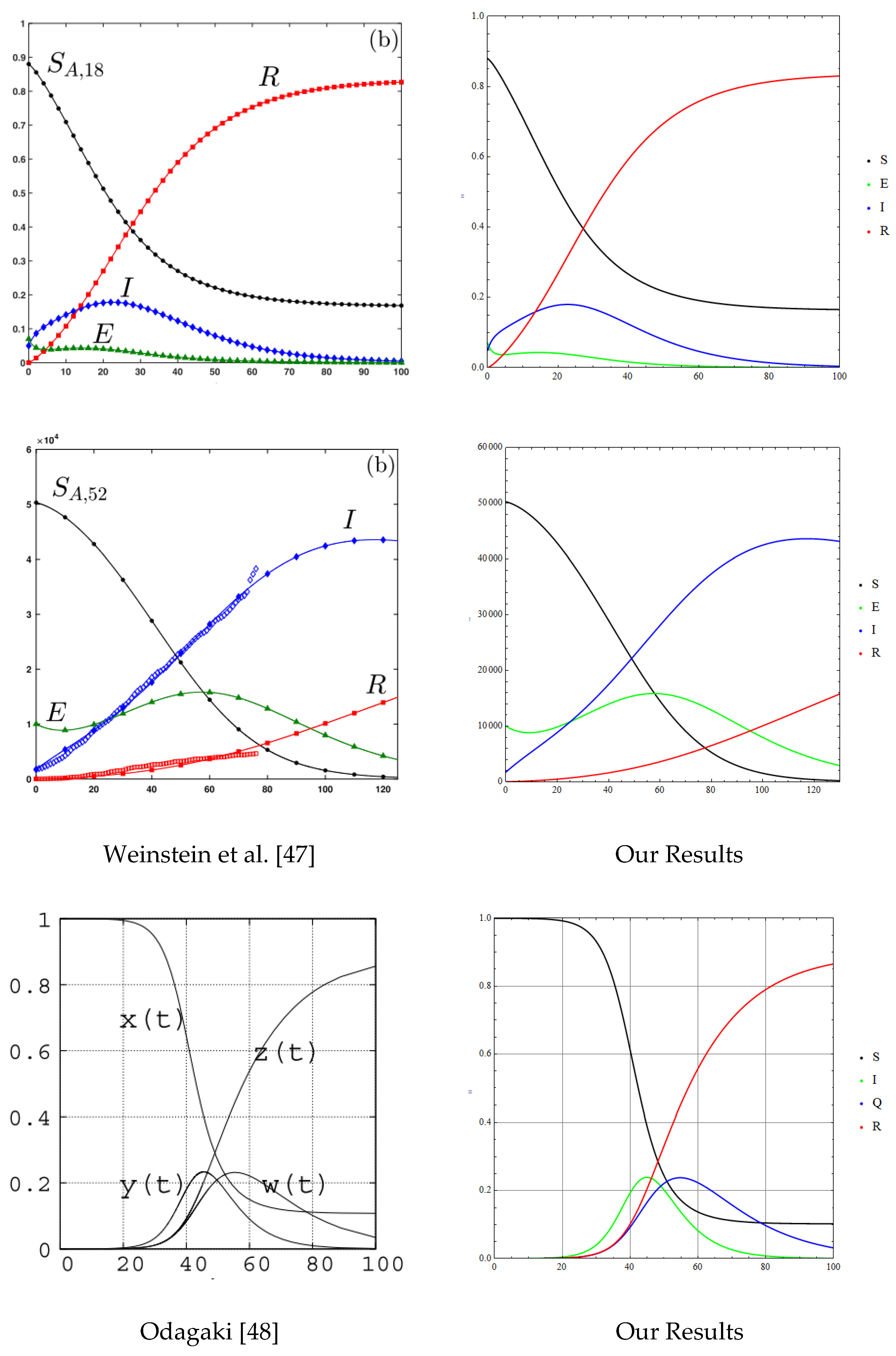
The well-known Euler method was utilized in this research to solve system (2) along with the initial conditions. The numerical method's specifics are described in Burden et al. [46]. To validate the numerical code, multiple validation steps were undertaken. Initially, three COVID-19 models, namely SIR, SEIR, and SIQR, were examined, which were presented by Turkyilmazoglu [14], Weinstein et al. [47], and Odagaki [48], respectively. The outcomes are illustrated in Figure 1(a, b, c), and they demonstrate that our results are in excellent agreement with those of Turkyilmazoglu [14], Weinstein et al. [47], and Odagaki [48]. Our findings suggest that we can continue the research with our proposed model, as there is good agreement.

4.2. Effect of Vaccines

4.2.1. Effect of COVID-19 Vaccine Coverage

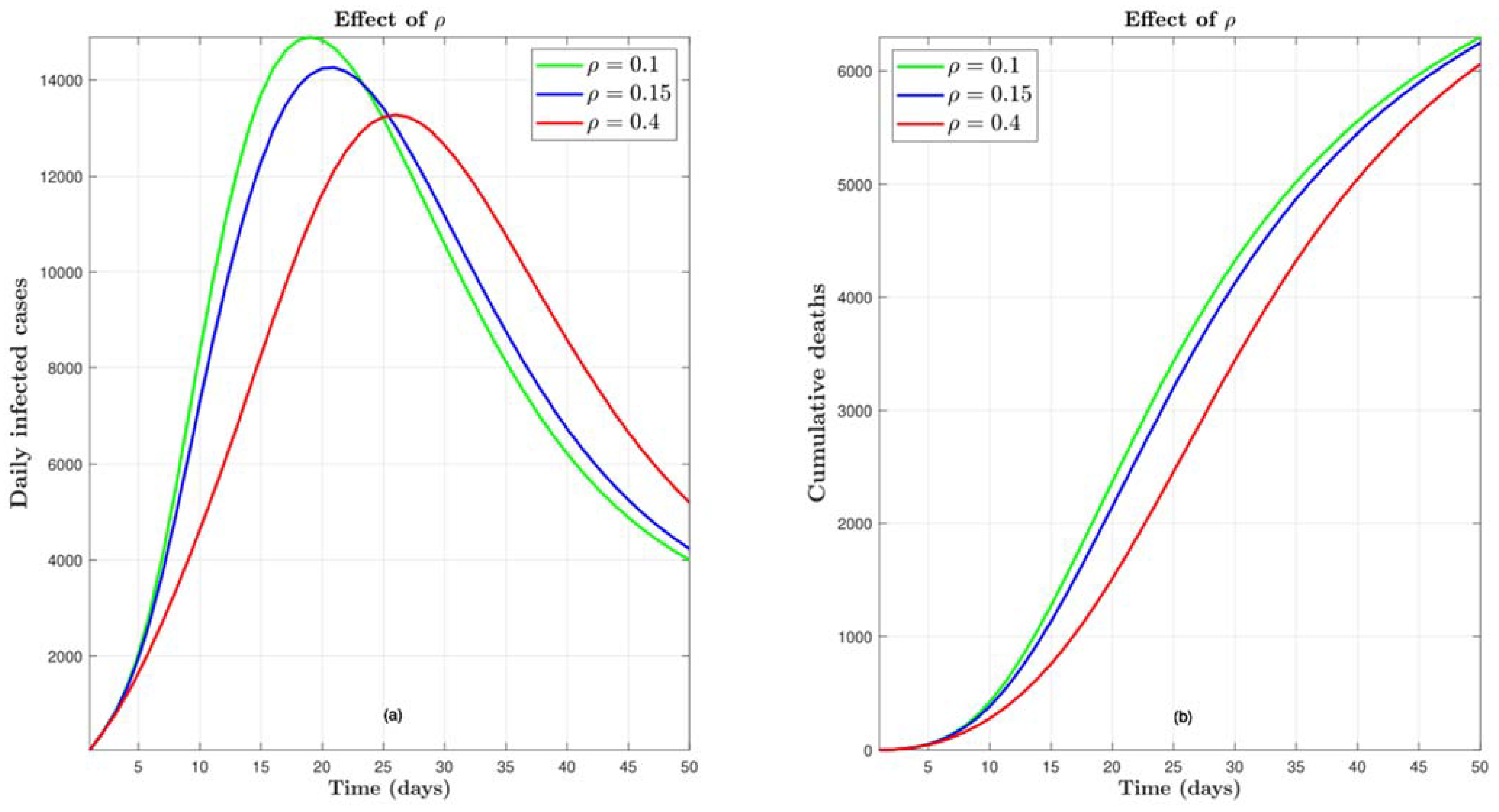
The results are presented in Figure 2(a, b), which demonstrates the effects of vaccination coverage on reducing the number of infected individuals and deaths. According to the results, there is a significant decrease in the number of infected individuals and deaths as the number of vaccinated individual’s increases. Figure 2(a) specifically shows that the peak of daily infected cases decreases by 11% when vaccination coverage increases from 10% to 40%. This means that a higher vaccination coverage could lead to fewer individuals being infected daily, thereby reducing the overall burden on the healthcare system and decreasing the risk of transmission to others. Overall, results suggest that increasing vaccination coverage can significantly reduce the number of COVID-19 infections and deaths, which is critical in controlling the pandemic's spread.

4.2.2. Effect of COVID-19 Vaccine Efficacy

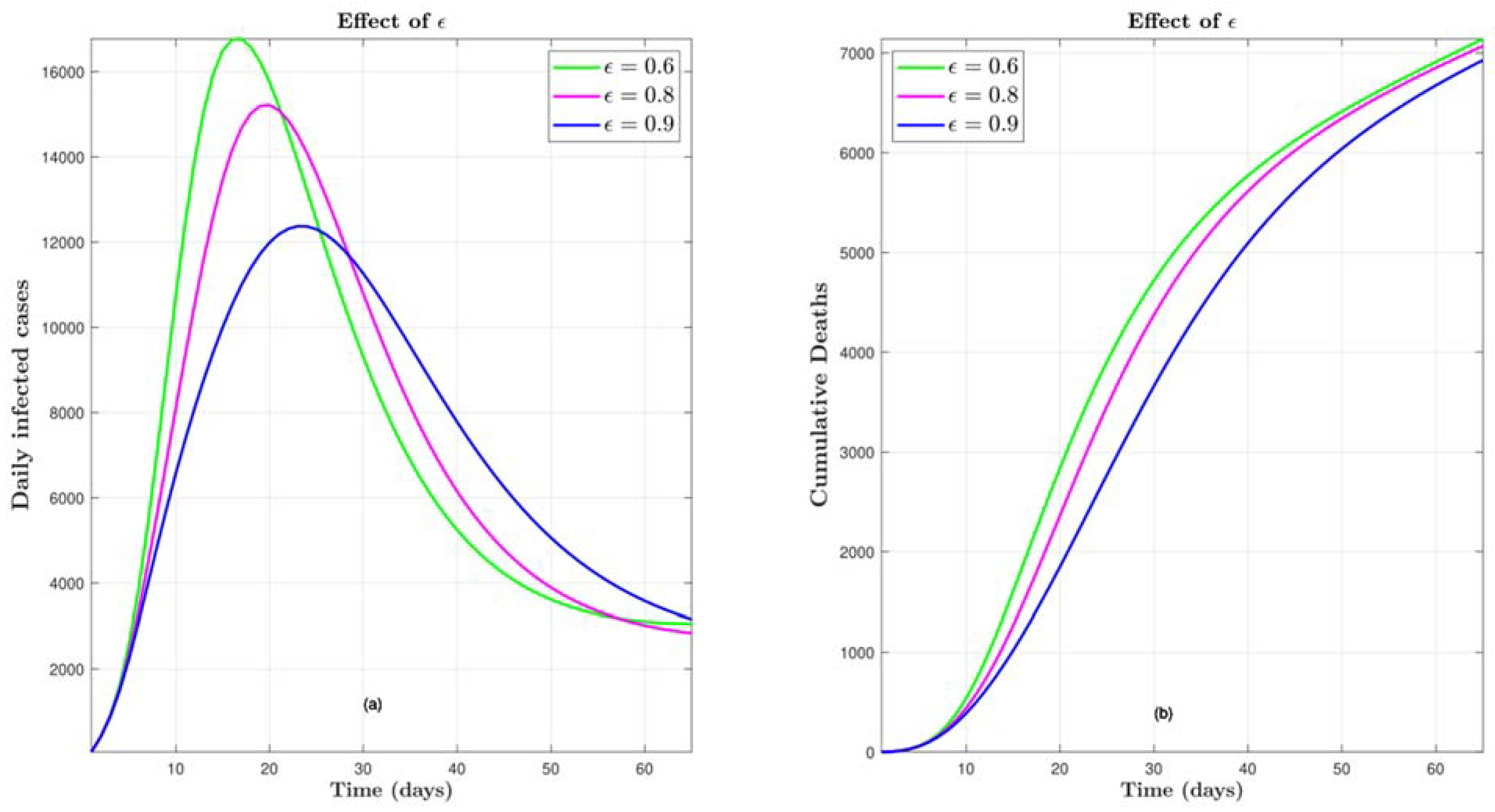
Results are presented in Figure 3(a, b), which shows the effects of vaccine efficacy on reducing the number of daily infected cases and deaths. According to the results, there is a considerable reduction in the number of daily infected cases and deaths as vaccine efficacy increases. For example, Figure 3(a) shows that when vaccine efficacy increases from 60% to 80%, the peak of daily infected cases drops from 16750 to 15210, representing a 10% decrease in the number of daily infected cases. This indicates that vaccines with higher efficacy can significantly reduce the spread of the virus, leading to fewer infections and less severe disease outcomes. These results are crucial in determining the effectiveness of various vaccines and their potential impact on the control of the COVID-19 pandemic. The simulation results suggest that vaccines with higher efficacy could play a vital role in reducing the number of COVID-19 cases and deaths, especially in populations with lower vaccination coverage. In summary, results presented in Figure 3(a, b) indicate that the impact of vaccine efficacy is significant in reducing the number of daily infected cases and deaths, emphasizing the importance of using vaccines with higher efficacy in controlling the spread of the COVID-19 virus.

4.3. Effect of τ

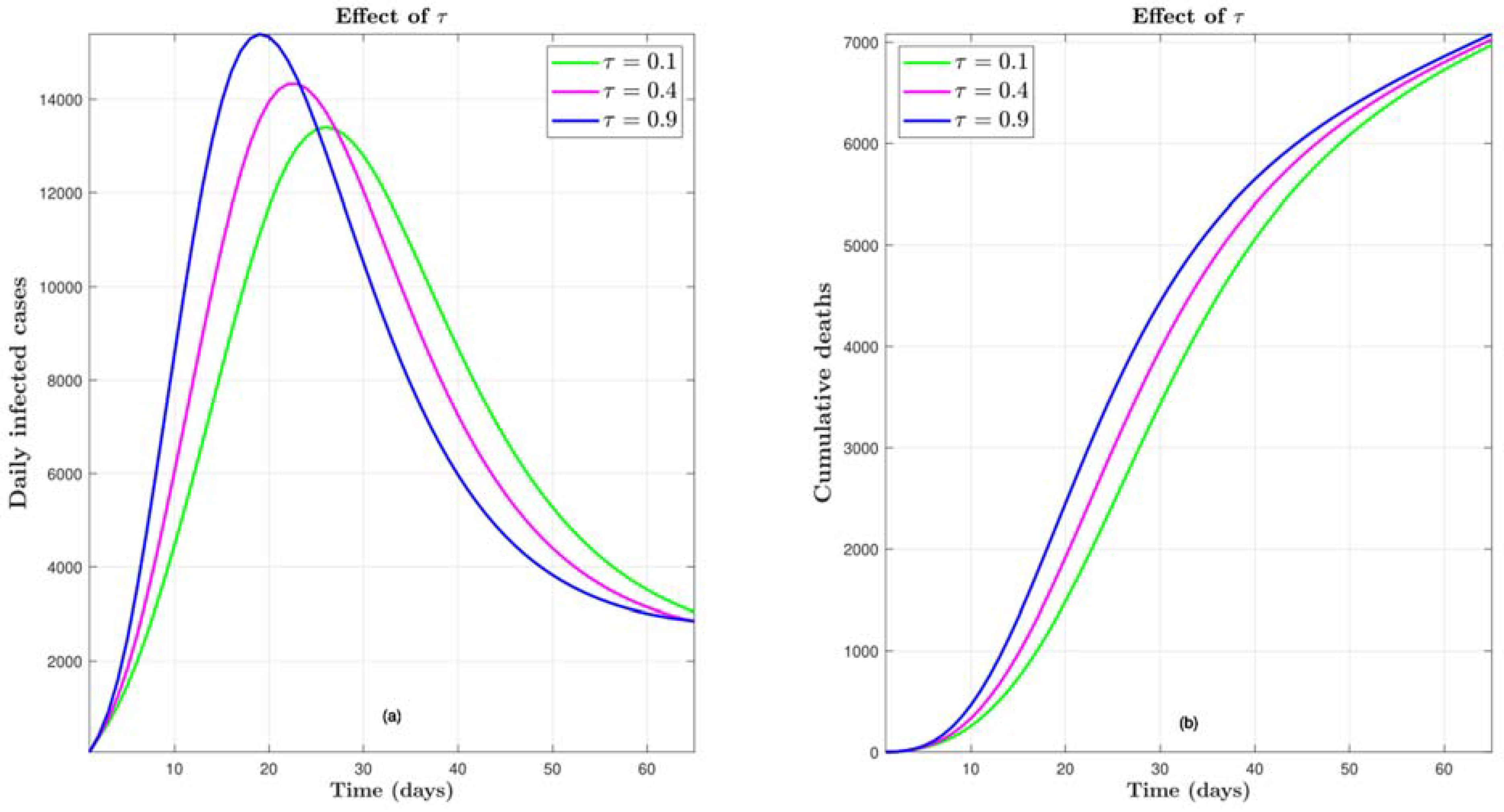
The simulation results for different values of τ are displayed in Figure 4(a, b). These figures demonstrate that both the daily infected cases and cumulative deaths rise with an increase in τ. For example, in Figure 4(a), when τ equals 0.1, the peak of daily infected cases is 13,400. However, when τ is 0.4, the peak of daily infected cases increases to 14,430, resulting in an 8% rise in the peak of daily infected cases. Similar patterns can be observed in Figure 4(b).

4.4. Effect of ω

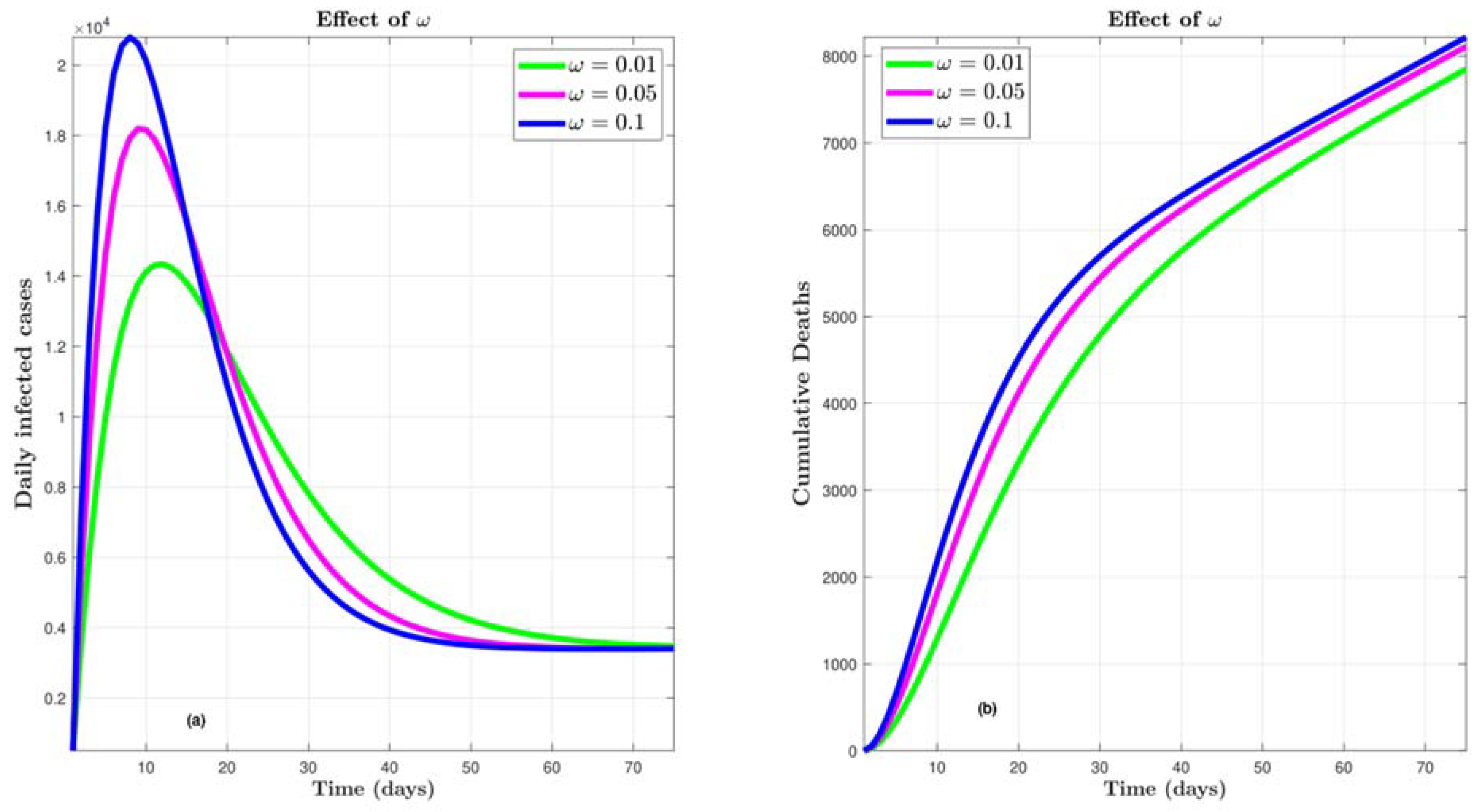
Numerical simulation is conducted to evaluate the impact of ω on disease transmission. The simulation results for model (2) with varying values of ω are presented in Figure 5(a, b). These figures illustrate that the complexity of COVID-19 increases as ω rises. For example, Figure 5(a) indicates a 27% increase in the peak of daily infected cases when ω increases from 0.01 to 0.05.

4.5. Effect of κ 1

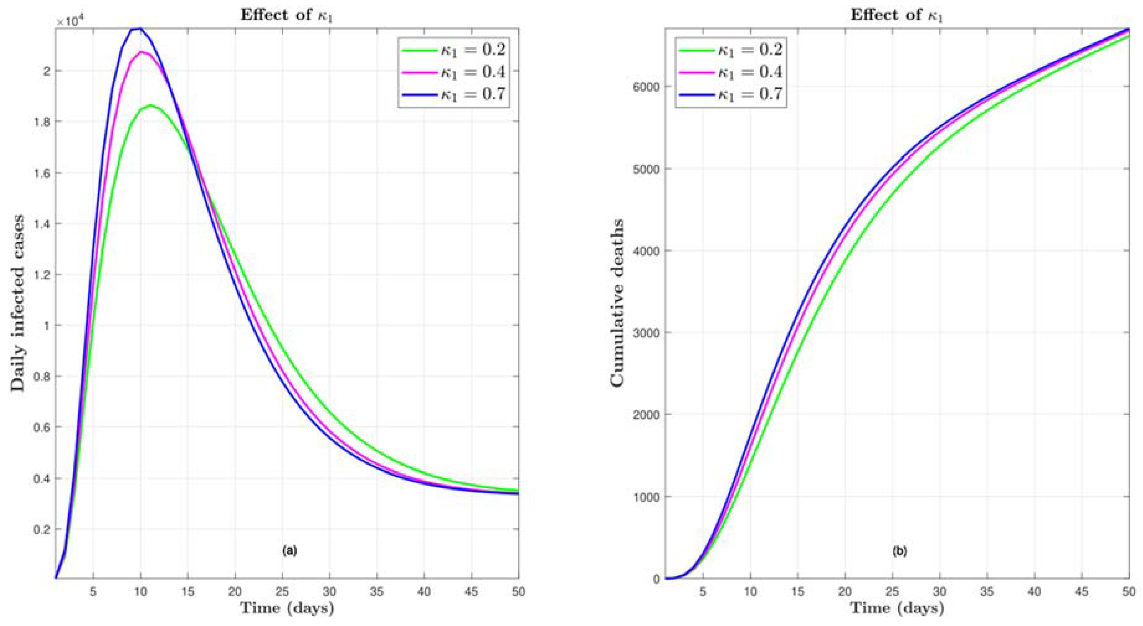
Furthermore, numerical simulation is carried out to investigate the impact of κ 1 . The simulation results are displayed in Figure 6(a, b), indicating that an increase in κ 1 leads to a rise in both daily infected cases and cumulative deaths. For instance, Figure 6(a) reveals a 16% decrease in the peak value of daily infected cases when κ 1 increases from 0.2 to 0.4. Moreover, the peak value of daily infected cases further increases by 5% when κ 1 changes from 0.4 to 0.7. Figure 6(b) demonstrates a similar trend.

4.6. Effect of κ 2

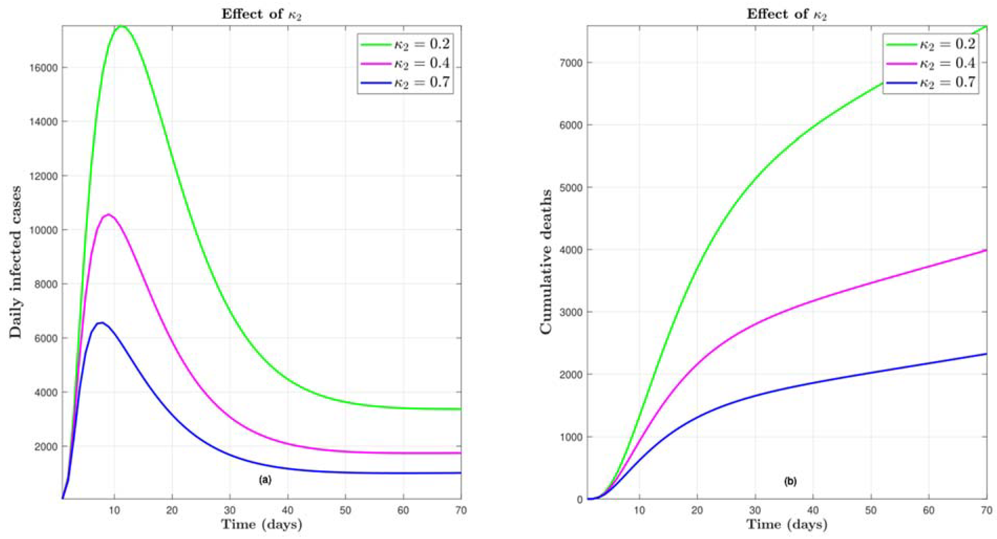
To evaluate the impact of κ 2 , numerical simulation is performed using model (2) with varying values of κ 2 . The simulation results are presented in Figure 7, indicating that an increase in κ 2 leads to a decrease in both daily infected cases and cumulative deaths. For example, in Figure 7(a), when κ 2 = 0.2, the peak of daily infected cases is 17540. However, when κ 2 = 0.4, the peak of daily infected cases reduces to 10570, resulting in a 40% decrease in the peak value of daily infected cases. The same trend is observed in Figure 7(b).

4.7. Effect of Transmission Rate

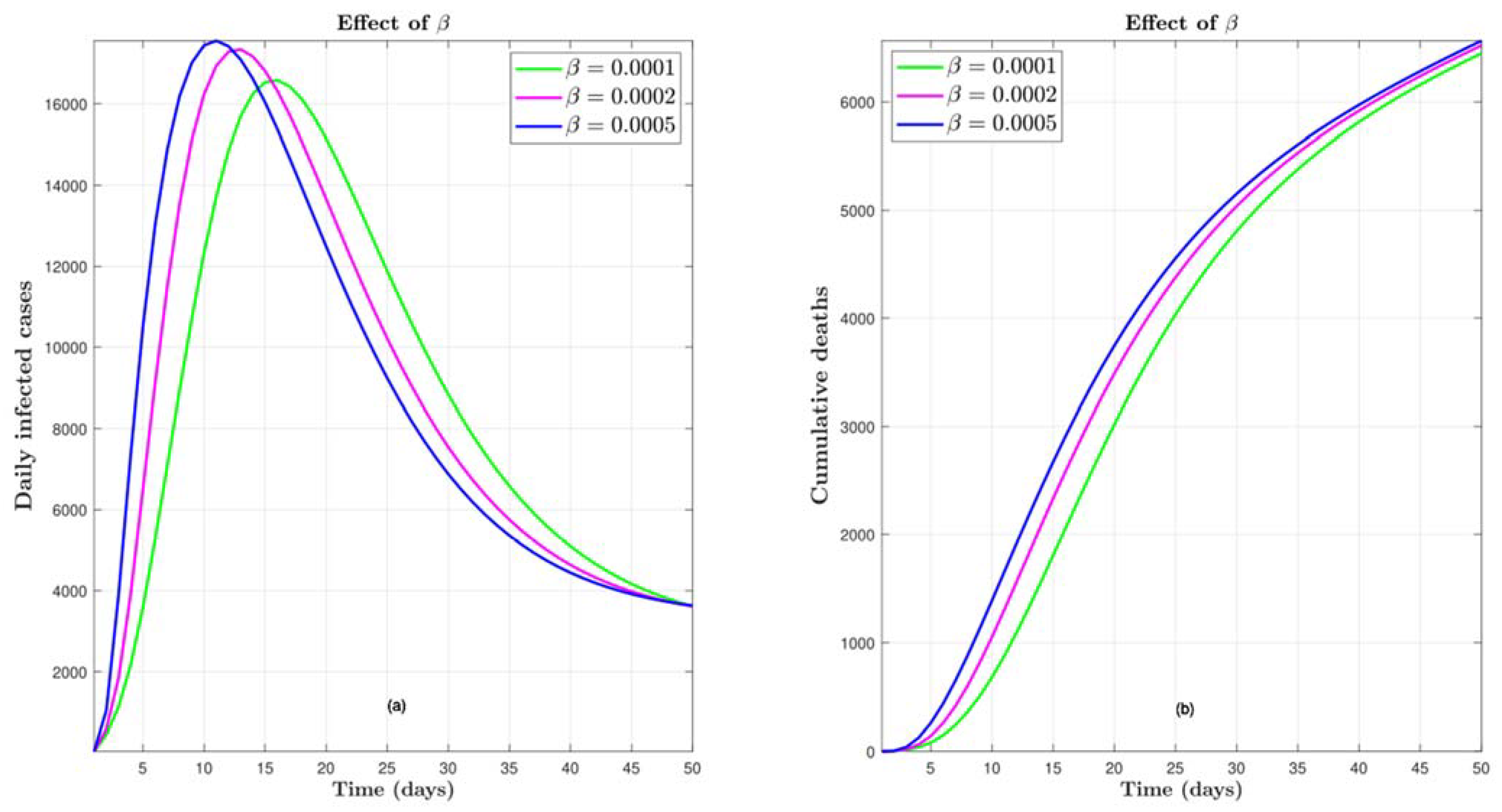
The figures 8(a, b) indicate that strict adherence to social distancing measures can play an important role in controlling the spread of COVID-19 infections and associated deaths. Figure 8(a) shows that when the contact rate is reduced from 0.0005 to 0.0002, the peak of daily infected cases decreases from 17,600 to 17,300, representing a 2% decrease in the peak value of daily infected cases. A similar pattern is observed in Figure 8(b). These results suggest that reducing the effective contact rate by adhering to social distancing measures can be an effective strategy for controlling the spread of COVID-19. The numerical simulations provide important insights into the impact of different variables on disease transmission and can inform public health policies and interventions aimed at reducing the spread of the virus.

5. Conclusion

Controlling the transmission of COVID-19, a highly infectious and deadly disease, is crucial. Mathematical models can provide insights into disease dynamics and potential methods for control. Thus, a new mathematical model has been developed to address these concerns. The first step in our analysis was to examine the model theoretically. We established the positivity and boundedness of the model's solutions, and calculated its basic reproduction number. Additionally, we used a theorem to demonstrate the local asymptotic stability of the DFE when the basic reproduction number is less than one. The study further demonstrated the local asymptotic stability of the EEP when the reproduction number is greater than one. The existence of the backward bifurcation phenomenon was examined using center manifold theory, revealing that it may occur under specific conditions. Additionally, the model's globally asymptotic stability was demonstrated for the DFE under certain conditions when the basic reproduction number is less than one.
In addition to the theoretical analysis, we conducted numerical simulations to further validate our findings and to explore the impact of various parameters on the dynamics of the model. The simulations confirmed that widespread and effective vaccination can play a significant role in controlling the spread of COVID-19. The results also demonstrated that reducing the contact rate can be an effective strategy for decreasing the number of infections and deaths related to COVID-19. Specifically, our simulations showed that when highly effective vaccines were administered to a large portion of the population, the number of daily infected cases and deaths decreased significantly. Conversely, when the effective contact rate was reduced, the number of daily infected cases also decreased. These findings highlight the importance of implementing measures to reduce contact rates and promote vaccination as part of an effective strategy for controlling the spread of COVID-19.

References

  1. Barlow, N.S.; Weinstein, S.J. Accurate closed-form solution of the SIR epidemic model. Physica. D 2020, 408, 132540–132540. [Google Scholar] [CrossRef] [PubMed]
  2. Tomchin, D.A.; Fradkov, A.L. Prediction of the COVID-19 spread in Russia based on SIR and SEIR models of epidemics. IFAC PapersOnLine 2020, 53, 833–838. [Google Scholar] [CrossRef] [PubMed]
  3. Marinov, T.T.; Marinova, R.S. Dynamics of COVID-19 using inverse problem for coefficient identification in SIR epidemic models. Chaos, Solitons & Fractals: X 2020, 5, 100041–100041. [Google Scholar] [CrossRef]
  4. Neves, A.G.M.; Guerrero, G. Predicting the evolution of the COVID-19 epidemic with the A-SIR model: Lombardy, Italy and São Paulo state, Brazil. Physica. D 2020, 413, 132693–132693. [Google Scholar] [CrossRef]
  5. Alenezi, M.N.; Al-Anzi, F.S.; Alabdulrazzaq, H. Building a sensible SIR estimation model for COVID-19 outspread in Kuwait. Alexandria engineering journal 2021, 60, 3161–3175. [Google Scholar] [CrossRef]
  6. Din, R.u.; Algehyne, E.A. Mathematical analysis of COVID-19 by using SIR model with convex incidence rate. Results in physics 2021, 23, 103970–103970. [Google Scholar] [CrossRef]
  7. Malavika, B.; Marimuthu, S.; Joy, M.; Nadaraj, A.; Asirvatham, E.S.; Jeyaseelan, L. Forecasting COVID-19 epidemic in India and high incidence states using SIR and logistic growth models. Clinical epidemiology and global health 2021, 9, 26–33. [Google Scholar] [CrossRef]
  8. Kozyreff, G. Hospitalization dynamics during the first COVID-19 pandemic wave: SIR modelling compared to Belgium, France, Italy, Switzerland and New York City data. Infectious disease modelling 2021, 6, 398–404. [Google Scholar] [CrossRef]
  9. Campos, E.L.; Cysne, R.P.; Madureira, A.L.; Mendes, G.L.Q. Multi-generational SIR modeling: Determination of parameters, epidemiological forecasting and age-dependent vaccination policies. Infectious disease modelling 2021, 6, 751–765. [Google Scholar] [CrossRef]
  10. Kudryashov, N.A.; Chmykhov, M.A.; Vigdorowitsch, M. Analytical features of the SIR model and their applications to COVID-19. Applied Mathematical Modelling 2021, 90, 466–473. [Google Scholar] [CrossRef]
  11. Cooper, I.; Mondal, A.; Antonopoulos, C.G. A SIR model assumption for the spread of COVID-19 in different communities. Chaos, solitons and fractals 2020, 139, 110057–110057. [Google Scholar] [CrossRef] [PubMed]
  12. Nesteruk, I. Statistics-Based Procedure of Parameter Identification for the Classical SIR Model; Springer: Singapore, 2021; pp. 33–36. [Google Scholar] [CrossRef]
  13. Nesteruk, I. Applications of the General SIR Model for Calculations of the COVID-19 Epidemic Waves in Ukraine; Springer: Singapore, 2021; pp. 141–146. [Google Scholar] [CrossRef]
  14. Turkyilmazoglu, M. Explicit formulae for the peak time of an epidemic from the SIR model. Physica. D 2021, 422, 132902–132902. [Google Scholar] [CrossRef] [PubMed]
  15. Anand, N.; Sabarinath, A.; Geetha, S.; Somanath, S. Predicting the Spread of COVID-19 Using SIR Model Augmented to Incorporate Quarantine and Testing. Transactions of the Indian National Academy of Engineering (Online) 2020, 5, 141–148. [Google Scholar] [CrossRef]
  16. Lounis, M.; Bagal, D.K. Estimation of SIR model’s parameters of COVID-19 in Algeria. Bulletin of the National Research Centre 2020, 44, 180–180. [Google Scholar] [CrossRef]
  17. Ramos, A.M.; Ferrández, M.R.; Vela-Pérez, M.; Kubik, A.B.; Ivorra, B. A simple but complex enough θ-SIR type model to be used with COVID-19 real data. Application to the case of Italy. Physica. D 2021, 421, 132839–132839. [Google Scholar] [CrossRef] [PubMed]
  18. Shahrear, P.; Rahman, S.M.S.; Nahid, M.M.H. Prediction and mathematical analysis of the outbreak of coronavirus (COVID-19) in Bangladesh. Results in Applied Mathematics 2021, 10, 100145–100145. [Google Scholar] [CrossRef] [PubMed]
  19. Uddin, M.B.; Hasan, M.; Harun-Al-Rashid, A.; Ahsan, M.I.; Imran, M.A.S.; Ahmed, S.S.U. Ancestral origin, antigenic resemblance and epidemiological insights of novel coronavirus (SARS-CoV-2): Global burden and Bangladesh perspective. Infection, genetics and evolution 2020, 84, 104440–104440. [Google Scholar] [CrossRef]
  20. Ahmed, J.; Jaman, M.H.; Saha, G.; Ghosh, P. Effect of environmental and socio-economic factors on the spreading of COVID-19 at 70 cities/provinces. Heliyon 2021, 7, e06979–e06979. [Google Scholar] [CrossRef]
  21. Alrabaiah, H.; Arfan, M.; Shah, K.; Mahariq, I.; Ullah, A. A comparative study of spreading of novel corona virus disease by ussing fractional order modified SEIR model. Alexandria Engineering Journal 2021, 60, 573–585. [Google Scholar] [CrossRef]
  22. López, L.; Rodó, X. A modified SEIR model to predict the COVID-19 outbreak in Spain and Italy: Simulating control scenarios and multi-scale epidemics. Results in physics 2021, 21, 103746–103746. [Google Scholar] [CrossRef]
  23. Hussain, T.; Ozair, M.; Ali, F.; Rehman, S.u.; Assiri, T.A.; Mahmoud, E.E. Sensitivity analysis and optimal control of COVID-19 dynamics based on SEIQR model. Results in physics 2021, 22, 103956–103956. [Google Scholar] [CrossRef] [PubMed]
  24. Li, J.; Zhong, J.; Ji, Y.-M.; Yang, F. A new SEIAR model on small-world networks to assess the intervention measures in the COVID-19 pandemics. Results in physics 2021, 25, 104283–104283. [Google Scholar] [CrossRef]
  25. Youssef, H.; Alghamdi, N.; Ezzat, M.A.; El-Bary, A.A.; Shawky, A.M. Study on the SEIQR model and applying the epidemiological rates of COVID-19 epidemic spread in Saudi Arabia. Infectious disease modelling 2021, 6, 678–692. [Google Scholar] [CrossRef]
  26. Yu, Z.; Arif, R.; Fahmy, M.A.; Sohail, A. Self organizing maps for the parametric analysis of COVID-19 SEIRS delayed model. Chaos, solitons and fractals 2021, 150, 111202–111202. [Google Scholar] [CrossRef]
  27. Adhikary, A.; Pal, A. A six compartments with time-delay model SHIQRD for the COVID-19 pandemic in India: During lockdown and beyond. Alexandria engineering journal 2022, 61, 1403–1412. [Google Scholar] [CrossRef]
  28. Akindeinde, S.O.; Okyere, E.; Adewumi, A.O.; Lebelo, R.S.; Fabelurin, O.O.; Moore, S.E. Caputo fractional-order SEIRP model for COVID-19 Pandemic. Alexandria engineering journal 2022, 61, 829–845. [Google Scholar] [CrossRef]
  29. Basnarkov, L. SEAIR Epidemic spreading model of COVID-19. Chaos, solitons and fractals 2021, 142, 110394–110394. [Google Scholar] [CrossRef] [PubMed]
  30. Khedher, N.b.; Kolsi, L.; Alsaif, H. A multi-stage SEIR model to predict the potential of a new COVID-19 wave in KSA after lifting all travel restrictions. Alexandria engineering journal 2021, 60, 3965–3974. [Google Scholar] [CrossRef]
  31. Pekpe, K.M.; Zitouni, D.; Gasso, G.; Dhifli, W.; Guinhouya, B.C. From SIR to SEAIRD: A novel data-driven modeling approach based on the Grey-box System Theory to predict the dynamics of COVID-19. Applied intelligence (Dordrecht, Netherlands) 2022, 52, 71–80. [Google Scholar] [CrossRef]
  32. Zhu, W.-j.; Shen, S.-f. An improved SIR model describing the epidemic dynamics of the COVID-19 in China. Results in physics 2021, 25, 104289–104289. [Google Scholar] [CrossRef]
  33. Chen, M.; Li, M.; Hao, Y.; Liu, Z.; Hu, L.; Wang, L. The introduction of population migration to SEIAR for COVID-19 epidemic modeling with an efficient intervention strategy. Information fusion 2020, 64, 252–258. [Google Scholar] [CrossRef] [PubMed]
  34. Contreras, S.; Villavicencio, H.A.; Medina-Ortiz, D.; Biron-Lattes, J.P.; Olivera-Nappa, Á. A multi-group SEIRA model for the spread of COVID-19 among heterogeneous populations. Chaos, solitons and fractals 2020, 136, 109925–109925. [Google Scholar] [CrossRef]
  35. Avila-Ponce de León, U.; Pérez, Á.G.C.; Avila-Vales, E. An SEIARD epidemic model for COVID-19 in Mexico: Mathematical analysis and state-level forecast. Chaos, solitons and fractals 2020, 140, 110165–110165. [Google Scholar] [CrossRef]
  36. Diekmann, O.; Heesterbeek, H.; Metz, J.A.J. On the definition and the computation of the basic reproduction ratio R0 in models for infectious diseases in heterogeneous populations. Journal of mathematical biology 1990, 28, 365–382. [Google Scholar] [CrossRef] [PubMed]
  37. van den Driessche, P.; Watmough, J. Reproduction numbers and sub-threshold endemic equilibria for compartmental models of disease transmission. Mathematical biosciences 2002, 180, 29–48. [Google Scholar] [CrossRef]
  38. Chavez, C.C.; Feng, Z.; Huang, W. On the computation of R0 and its role on global stability. Mathematical approaches for emerging and re-emerging infection diseases: an introduction 2002, 125, 31–65. [Google Scholar]
  39. Hethcote, H.W. The Mathematics of Infectious Diseases. SIAM review 2000, 42, 599–653. [Google Scholar] [CrossRef]
  40. Carr, J. Applications of Centre Manifold Theory; Applied Mathematical Sciences; Springer, 2012; Volume 35. [Google Scholar]
  41. Castillo-Chavez, C.; Song, B. Dynamical models of tuberculosis and their applications. Math. Biosci. Eng 2004, 1, 361–404. [Google Scholar] [CrossRef] [PubMed]
  42. La Salle, J.P., The stability of dynamical systems. 1976: SIAM.
  43. Ngonghala, C.N.; Iboi, E.; Eikenberry, S.; Scotch, M.; MacIntyre, C.R.; Bonds, M.H.; Gumel, A.B. Mathematical assessment of the impact of non-pharmaceutical interventions on curtailing the 2019 novel Coronavirus. Mathematical biosciences 2020, 325, 108364–108364. [Google Scholar] [CrossRef]
  44. Saha, A.K.; Podder, C.N.; Niger, A.M. Dynamics of novel COVID-19 in the presence of Co-morbidity. Infectious disease modelling 2022, 7, 138–160. [Google Scholar] [CrossRef]
  45. Mancuso, M.; Eikenberry, S.E.; Gumel, A.B. Will vaccine-derived protective immunity curtail COVID-19 variants in the US? Infectious disease modelling 2021, 6, 1110–1134. [Google Scholar] [CrossRef] [PubMed]
  46. Burden and Faires, Numerical Analysis. 2015: Cengage Learning.
  47. Weinstein, S.J.; Holland, M.S.; Rogers, K.E.; Barlow, N.S. Analytic solution of the SEIR epidemic model via asymptotic approximant. Physica. D 2020, 411, 132633–132633. [Google Scholar] [CrossRef] [PubMed]
  48. Odagaki, T. Exact properties of SIQR model for COVID-19. Physica A 2021, 564, 125564–125564. [Google Scholar] [CrossRef] [PubMed]
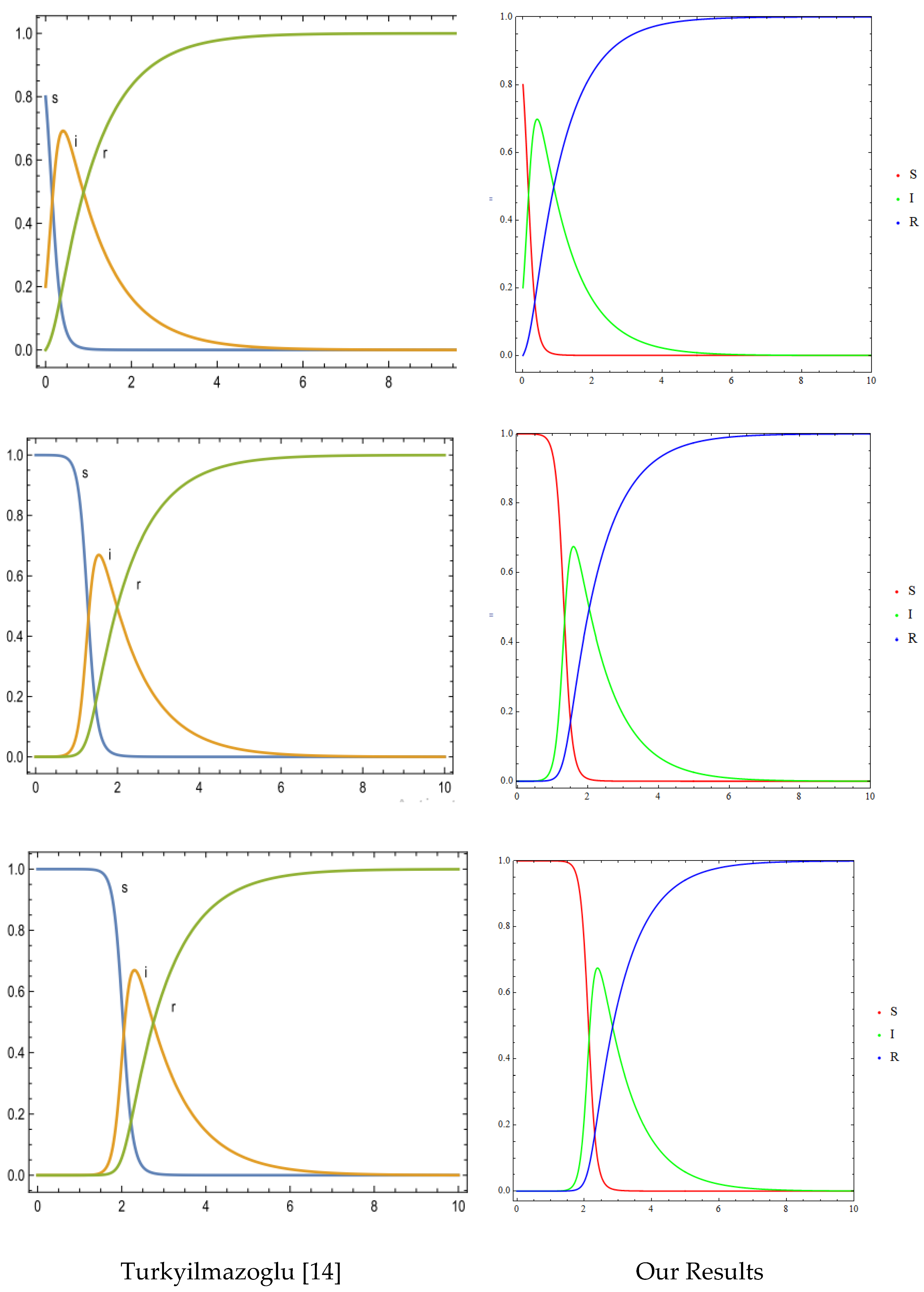
Figure 1. a: Results for SIR model; b: Results for SEIR model; c: Results for SIQR model.
Preprints 117386 g001aPreprints 117386 g001b
Figure 2. Numerical simulation of the model (2) showing the effect of vaccine coverage on the number of daily infected cases and cumulative deaths.
Preprints 117386 g002
Figure 3. Effect of vaccine efficacy on COVID-19 for the model (2) showing the number of daily infected cases and cumulative deaths.
Preprints 117386 g003
Figure 4. Simulation of the model (2) showing the effect of τ on the number of daily infected cases and cumulative deaths.
Preprints 117386 g004
Figure 5. Effect of ω on the number of daily COVID-infected cases and cumulative deaths.
Preprints 117386 g005
Figure 6. Numerical simulation showing the effect of κ 1 on the number of daily COVID-19 infected cases and cumulative deaths.
Preprints 117386 g006
Figure 7. Numerical simulation showing the effect of κ 2
Preprints 117386 g007
Figure 8. Simulation of the model (2) showing the effect of effective contact rate on the number of daily COVID-19 infected cases and cumulative deaths.
Preprints 117386 g008
Disclaimer/Publisher’s Note: The statements, opinions and data contained in all publications are solely those of the individual author(s) and contributor(s) and not of MDPI and/or the editor(s). MDPI and/or the editor(s) disclaim responsibility for any injury to people or property resulting from any ideas, methods, instructions or products referred to in the content.
Copyright: This open access article is published under a Creative Commons CC BY 4.0 license, which permit the free download, distribution, and reuse, provided that the author and preprint are cited in any reuse.
Prerpints.org logo

Preprints.org is a free preprint server supported by MDPI in Basel, Switzerland.

Subscribe

© 2024 MDPI (Basel, Switzerland) unless otherwise stated