Submitted:
06 September 2024
Posted:
06 September 2024
You are already at the latest version
Abstract
Keywords:
1. Introduction
- Visual interpretability of the cognitive continuum of knowledge learning human agents in TI works;
- Designing an Agent-based model of the complexity of content and contextual structure of TI work in a selected geographic area;
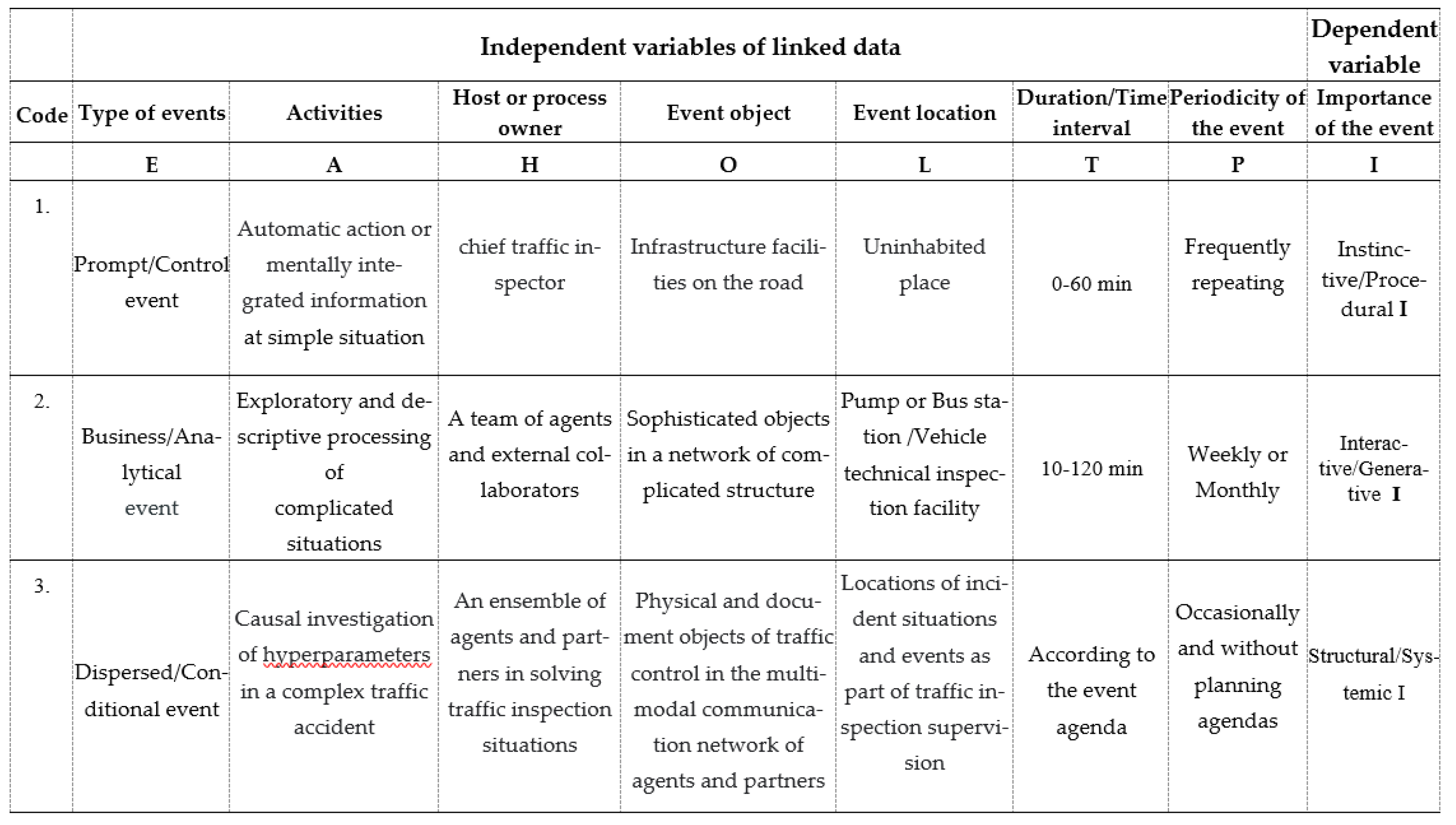
- Constructing an Event Execution Log (EEL) for TI tasks to research categorical variables in registers of related data for a defined research geographic area;
- Creating a research procedure with algorithmization of data cleaning operations and cleaned data processing in the EEL;
- Classification modeling of the significance of events in TI work based on machine learning techniques and Stacking ensemble.
2. Related Research
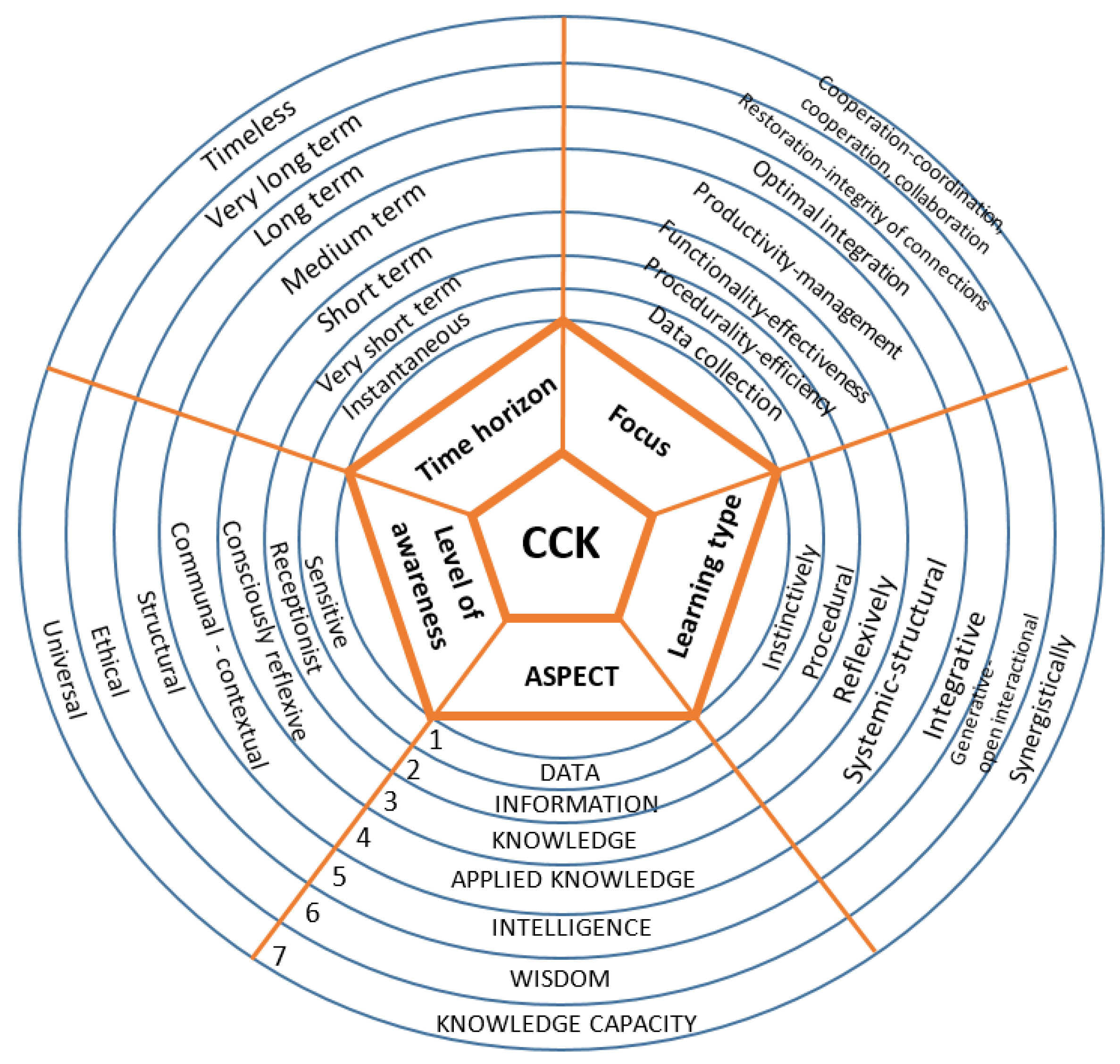
- Seven instances of knowledge aspect in the Cognitive Continuum of Knowledge (CCK), i.e., data (d), information (i), knowledge (K), applied knowledge (AK), intelligence (I), wisdom (W) and the capacity of knowledge (CK) for sharing in real situations of multimodal multi-agent communication in TI work.
- For the seven instances of knowledge aspect, the corresponding seven instances of the learning type indicator are identified as: instinctive learning, procedural learning, reflective learning, systemic-structural learning, integrative learning, generative-open interactive learning and synergistic learning [8];
- For the seven instances of knowledge aspect, the corresponding seven instances of the performance learning focus indicator are identified as: data collection (with feedback), procedurality (efficiency of information processing), functionality (effectiveness of information processing), productivity (reliability of management), optimal integration of knowledge repertoire, renewal-integrity of connections and cooperation in learning and sharing knowledge capacity in the form of 3C (3C – cooperation, coordination, collaboration) [8];
- For the seven instances of knowledge aspect, the corresponding seven instances of the learning time perspective indicator are identified as: current perspective, very short-term, short-term, medium-term, long-term, very long-term and timeless time perspective [8].
- For the seven instances of knowledge aspect, the corresponding seven instances of the indicator consciousness level, which develop through learning in different situations, are identified as: consciousness of feelings, sensory consciousness, reflective consciousness, contextual consciousness, structural consciousness, ethical and universal consciousness [8].
3. Material
3.1. Contemporary Research Frameworks for TI Work
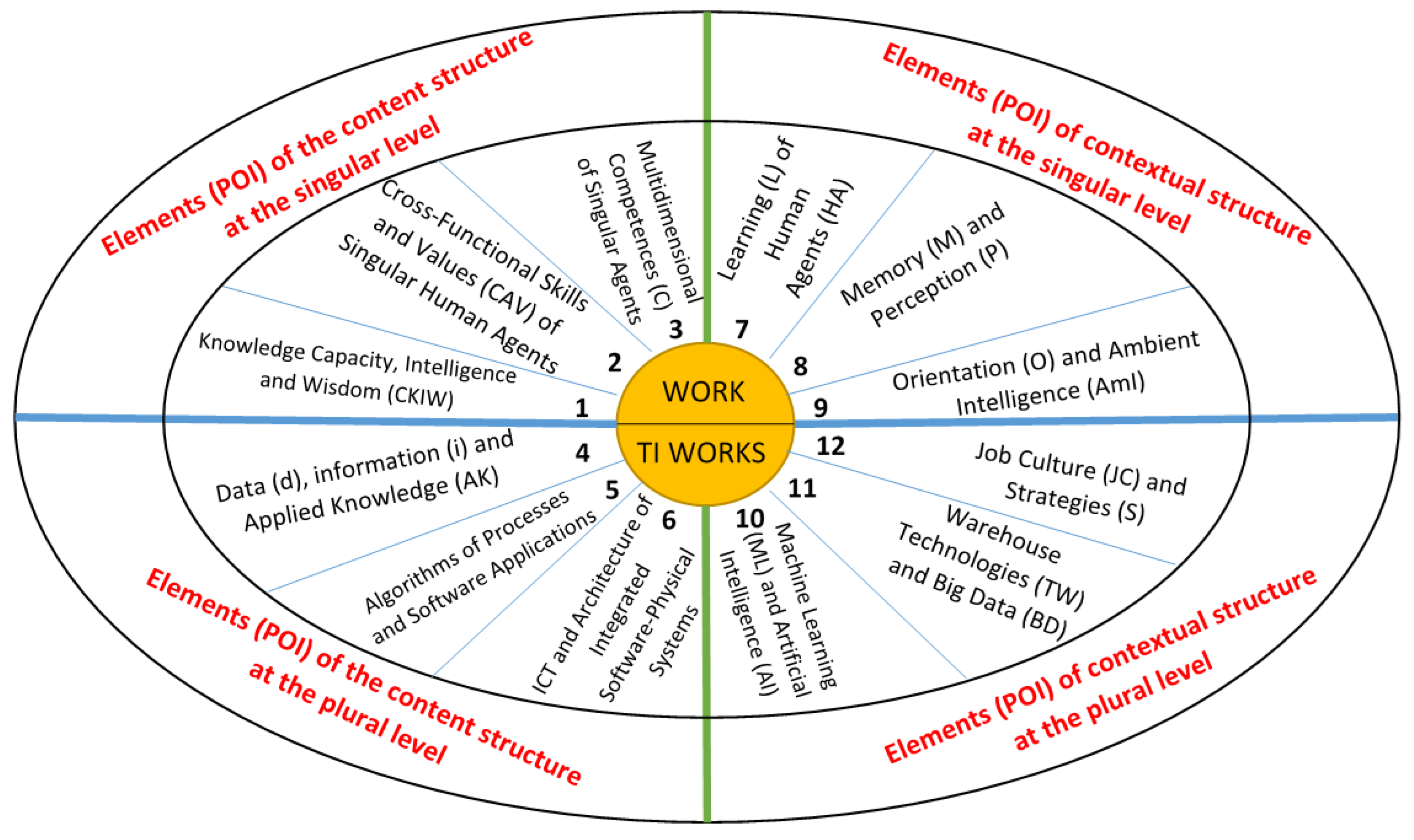
3.2. Agent-Based Model of the Complexity of Content and Contextual Structure of TI Work
3.2.1. Knowledge Capacity, Intelligence and Wisdom (CKIW)
3.2.2. Cross-Functional Skills and Values (CAV) of Singular Human Agents in TI Work
3.2.3. Multidimensional Competences (C) of Singular Agents in TI Work
3.2.4. Data (d), Information (i) and Applied Knowledge (AK) in TI Work
3.2.5. Algorithms of Processes and Software Applications in TI Work
3.2.6. Information and Communication Technology (ICT) and Architecture of Integrated Software-Physical Systems in TI Work
3.2.7. Learning of (L) Human Agents (HA) in TI Work
3.2.8. Memory (M) and Perception (P) in TI Operations
3.2.9. Orientations (O) and Ambient Intelligence (AmI) in TI Work
3.2.10. Machine Learning (ML) and Artificial Intelligence (AI) in TI Work
3.2.11. Warehouse Technologies (WT) and Big Data (BD) in IT Work
3.2.12. Job Culture (JC) and Strategies (S) in TI Work
4. Research Methodology
4.1. Exploratory On-Site Research of Event Execution in TI Work
4.2. Creation of the Event Execution Log of TI Tasks
4.3. Algorithmic Overview of the Research Methodology for Data Preprocessing (Data Cleaning) and Processing in the EEL
4.4. Data Cleaning Procedure in the Research Dataset Collected via EEL
- A smaller dataset often implies higher data quality,
- Eliminating irrelevant or incorrect data reduces noise in the dataset,
- Consistent data in a smaller dataset enables a more efficient process of machine learning model training without compromising model quality,
- Focus is on representative vectors,
- Achieving reduced overfitting,
- Simplified model validation and cost reduction.
5. Results of Creating a Machine Learning Model with Discussion
5.1. Creation of a Classification Model with all Observed Predictors
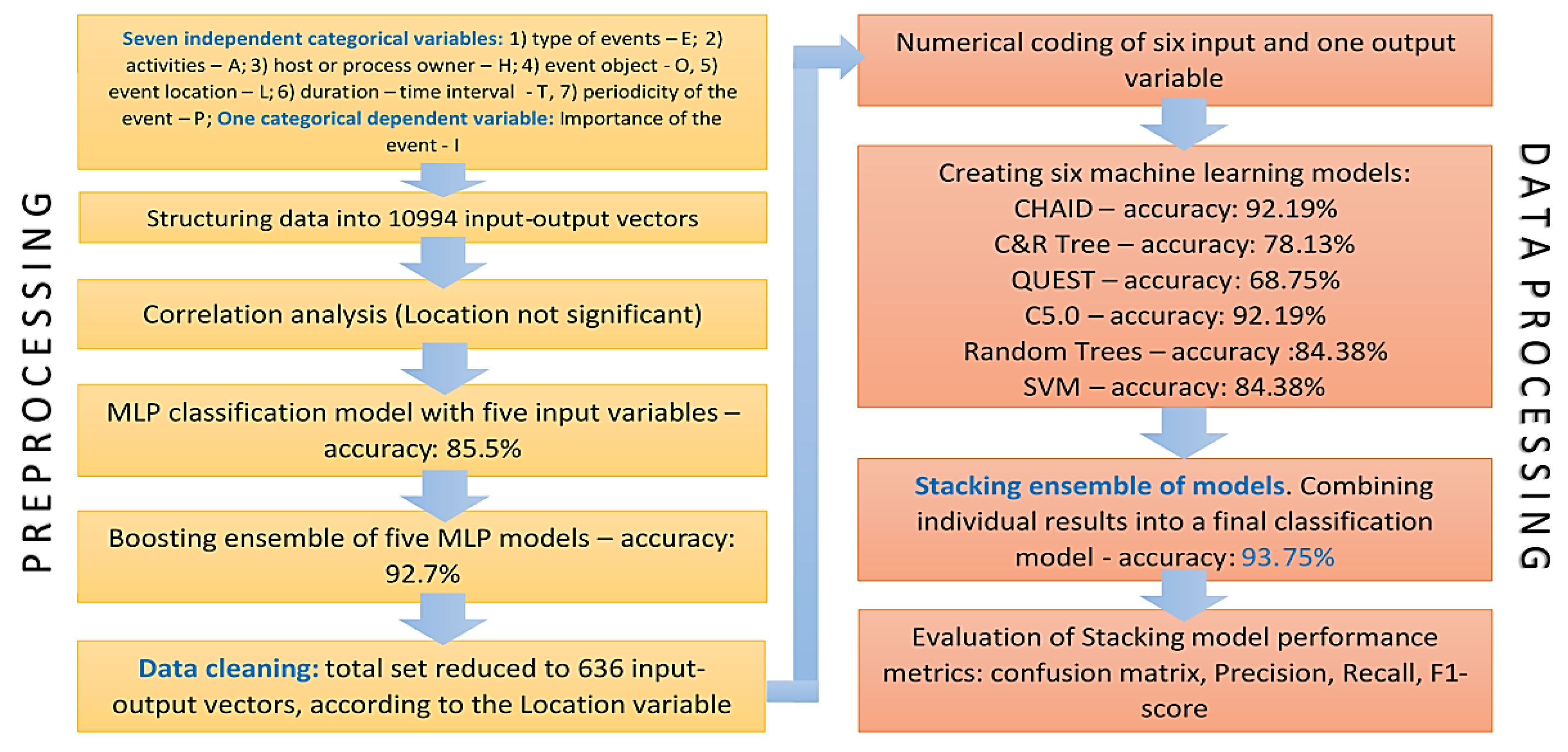
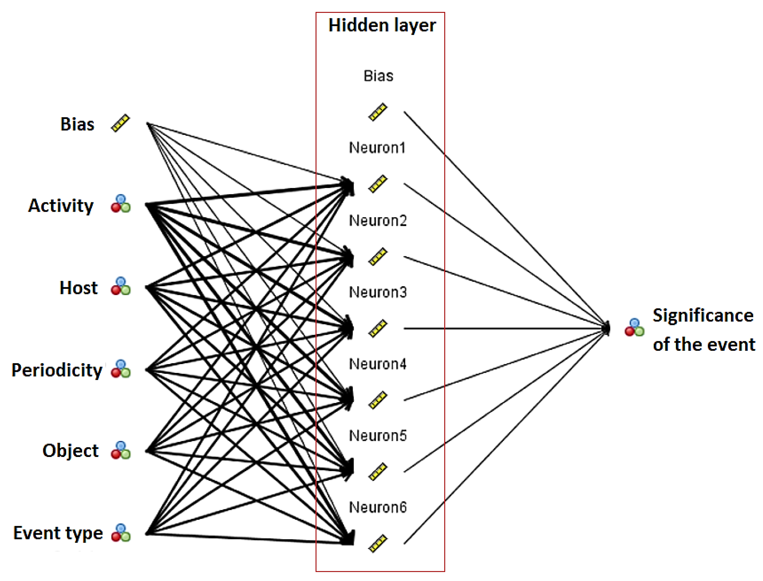
- The previous modeling with five predictors resulted in a model with greater interpretability. However, in many cases, a larger number of predictors can provide more information and thus enhance classification performance. Therefore, it is also necessary to model with a sixth independent variable, Location.
- To achieve better consistency, data cleaning according to the Location variable must be performed during preprocessing. It is assumed that each of the 636 categories of this variable represents key information, and reducing the total dataset to the same number of input-output vectors can help in better understanding the impact of each category on the model outcome. In addition, a smaller dataset offers certain advantages, some of which will be outlined below.
5.2. Results of Classification Modeling of Event Significance on the Cleaned Dataset
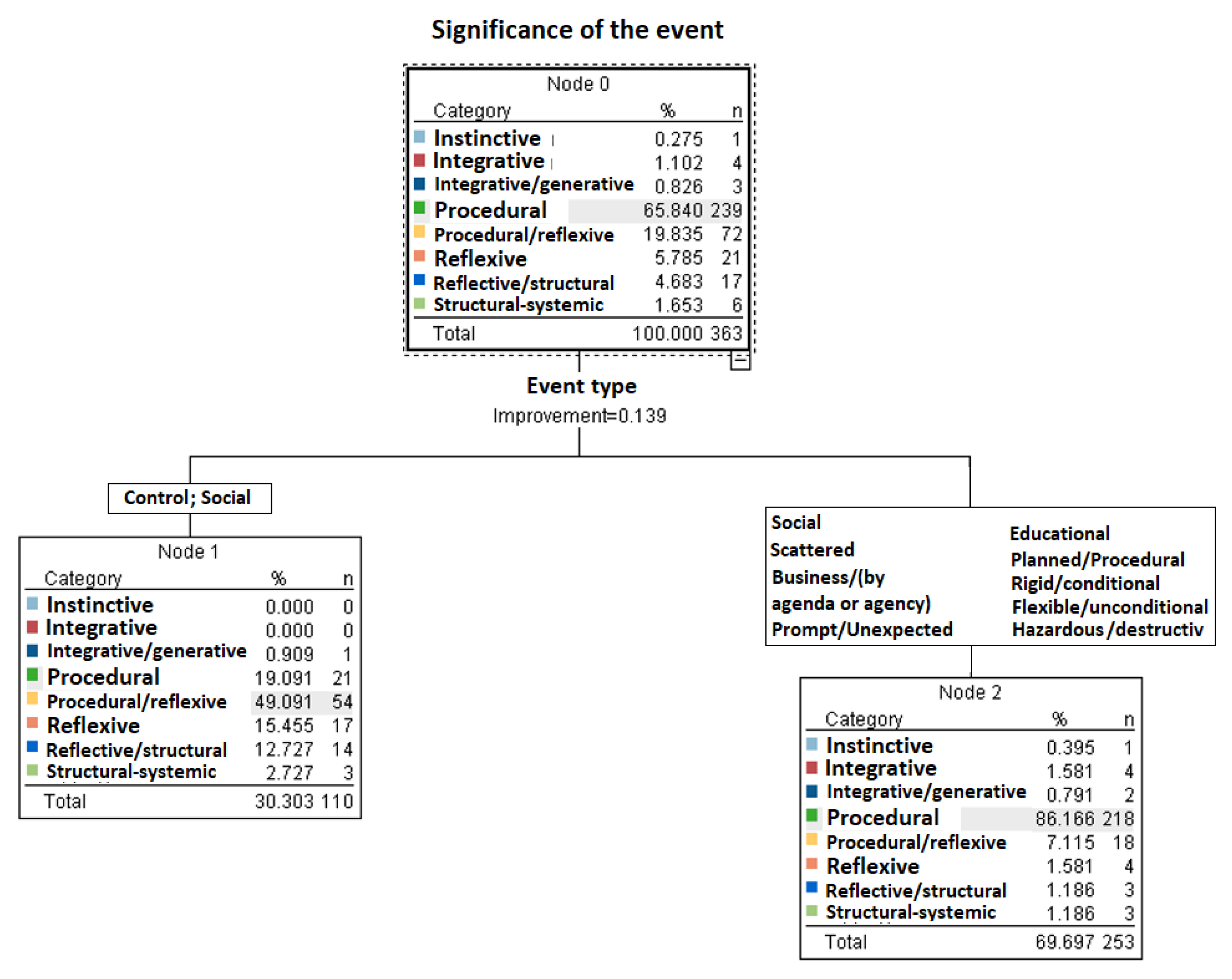
5.2.1. CHAID model
5.2.2. C&R Tree model
- Minimum records in parent branch – 2% of the total dataset,
- Minimum records in child branch – 1% of the total dataset.
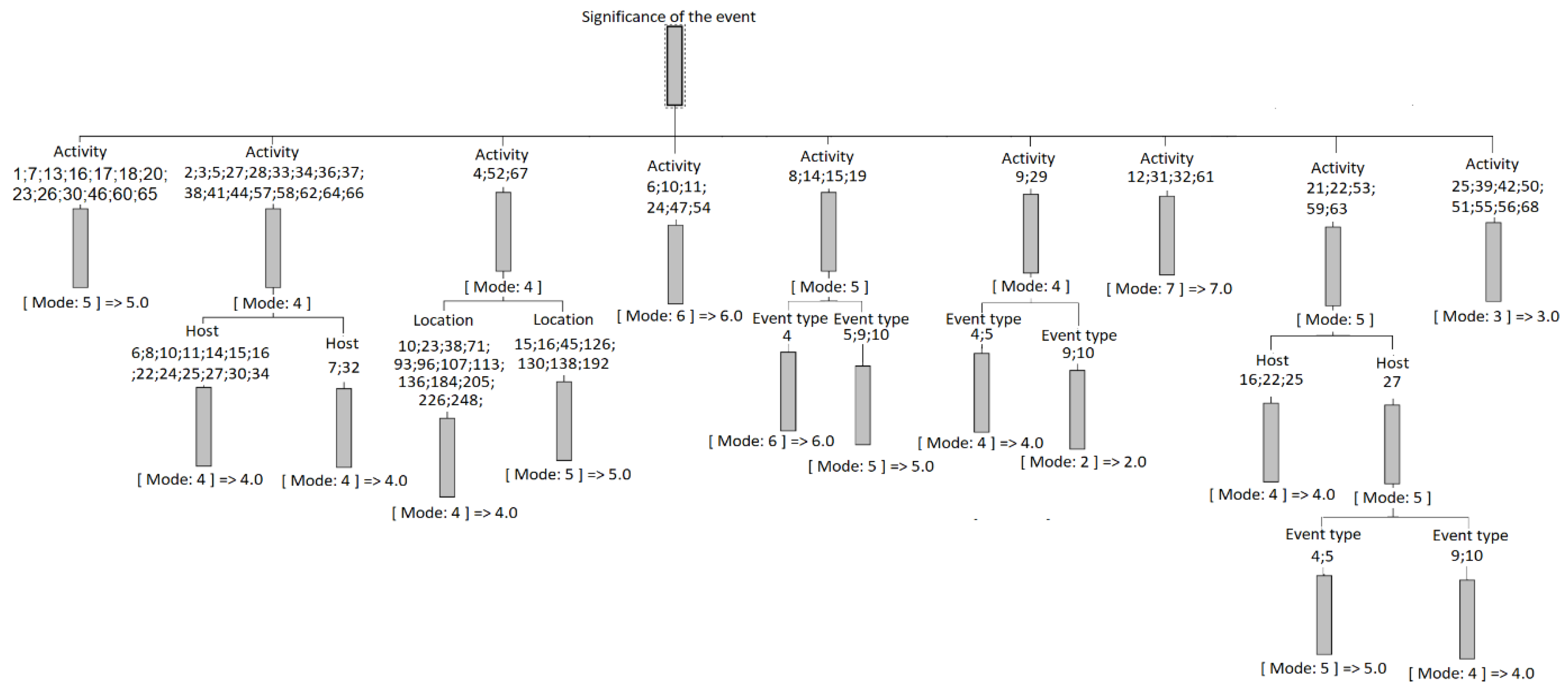
- Event_type in [ 2.000 4.000 5.000 ] [ Mode: 5 ] => 5.0
- Event_type in [ 1.000 3.000 6.000 7.000 8.000 9.000 10.000 11.000 12.000 14.000 15.000 ] [ Mode: 4 ] => 4.0
- Event_type in [ 2.000 4.000 5.000 ]: This means that the variable “Activity” has a value within the specified set of values: 2.000, 4.000, 5.000.
- [ Mode: 5 ]: “Mode” refers to the most frequent class in the dataset that satisfies the condition “Event_type in [ ... ]”. In this case, the most frequent class is 5.
- =>5.0: This part indicates the prediction or classification. If the “Activity” attribute has a value within the specified set of values, then the class prediction is 5.0.
5.2.3. QUEST model
- Left side of the rule: Mode: 4 suggests that the mode (most frequent value) for a particular node or data group is 4.
- Right side of the rule: => 4.0 indicates a prediction, i.e., if the mode is 4, the prediction or classification that the model provides is 4.0.
5.2.4. C5.0 model
5.2.5. Random Trees model
- Bagging (Bootstrap Aggregating): Multiple copies of the training set are generated by randomly sampling with backtracking. These copies, called bootstrap samples, are of the same size as the original dataset. A separate model, a member of the ensemble, is built on each of these samples [48].
- Random selection of input variables: For each decision (split) in the tree, not all independent variables are considered. Instead, only a random subset of the input variables is considered and impurity is measured only for these variables [48].
5.2.6. SVM model
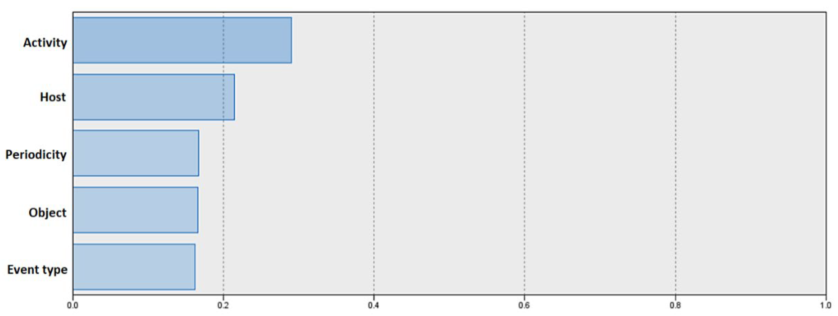
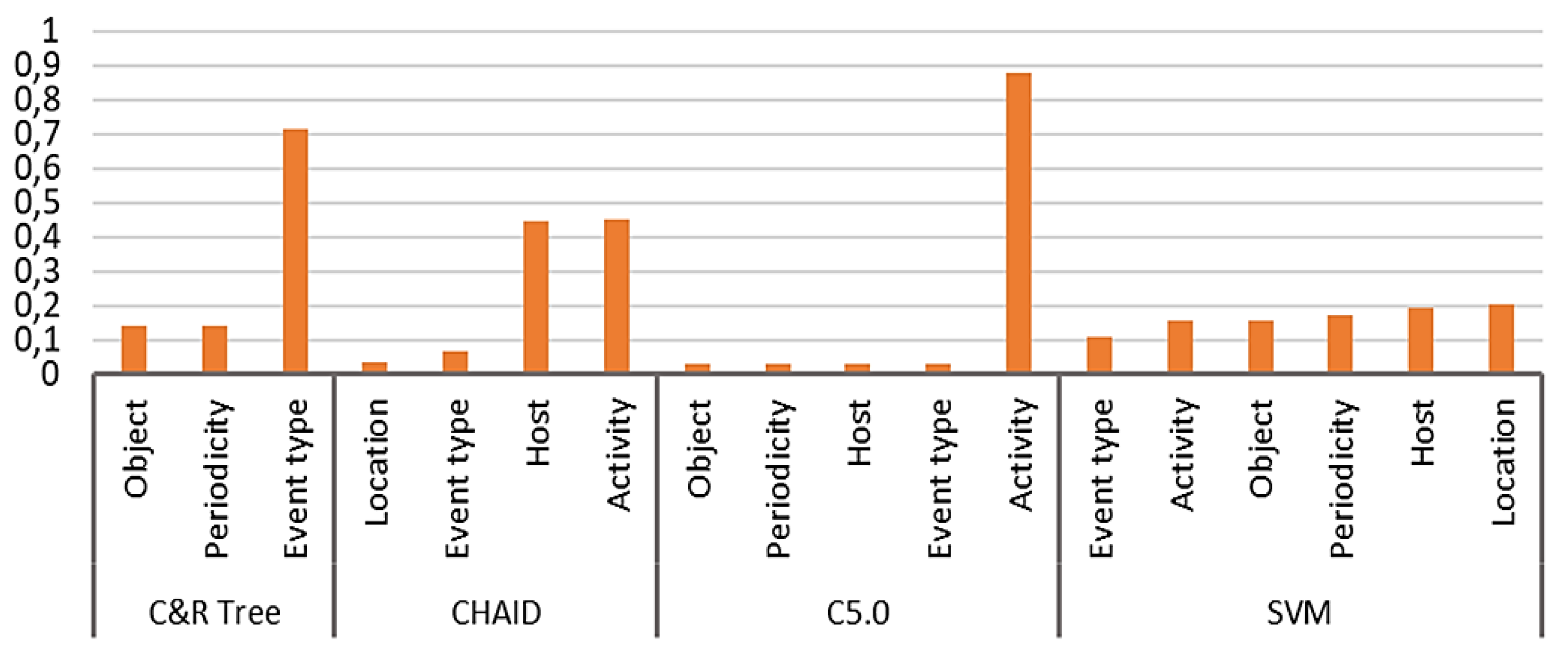
5.3. Predictor Importance Values for the Created Models
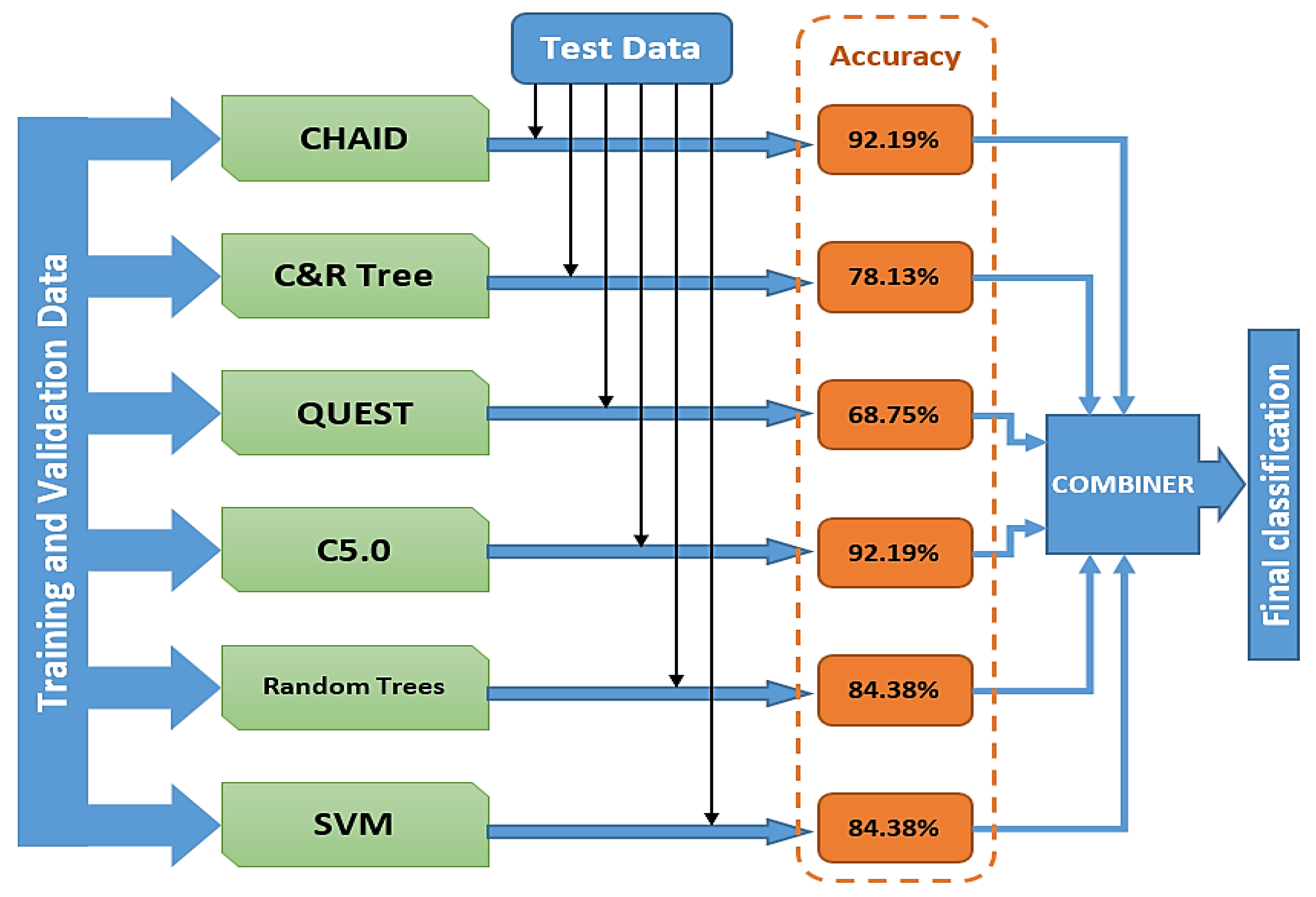
5.4. Stacking model ensemble for improving classification performance
- A set of classification models based on different algorithms,
- A set of classification models of the same type with different parameters and hyperparameters,
- A set of classification models of the same type on different samples from the dataset.
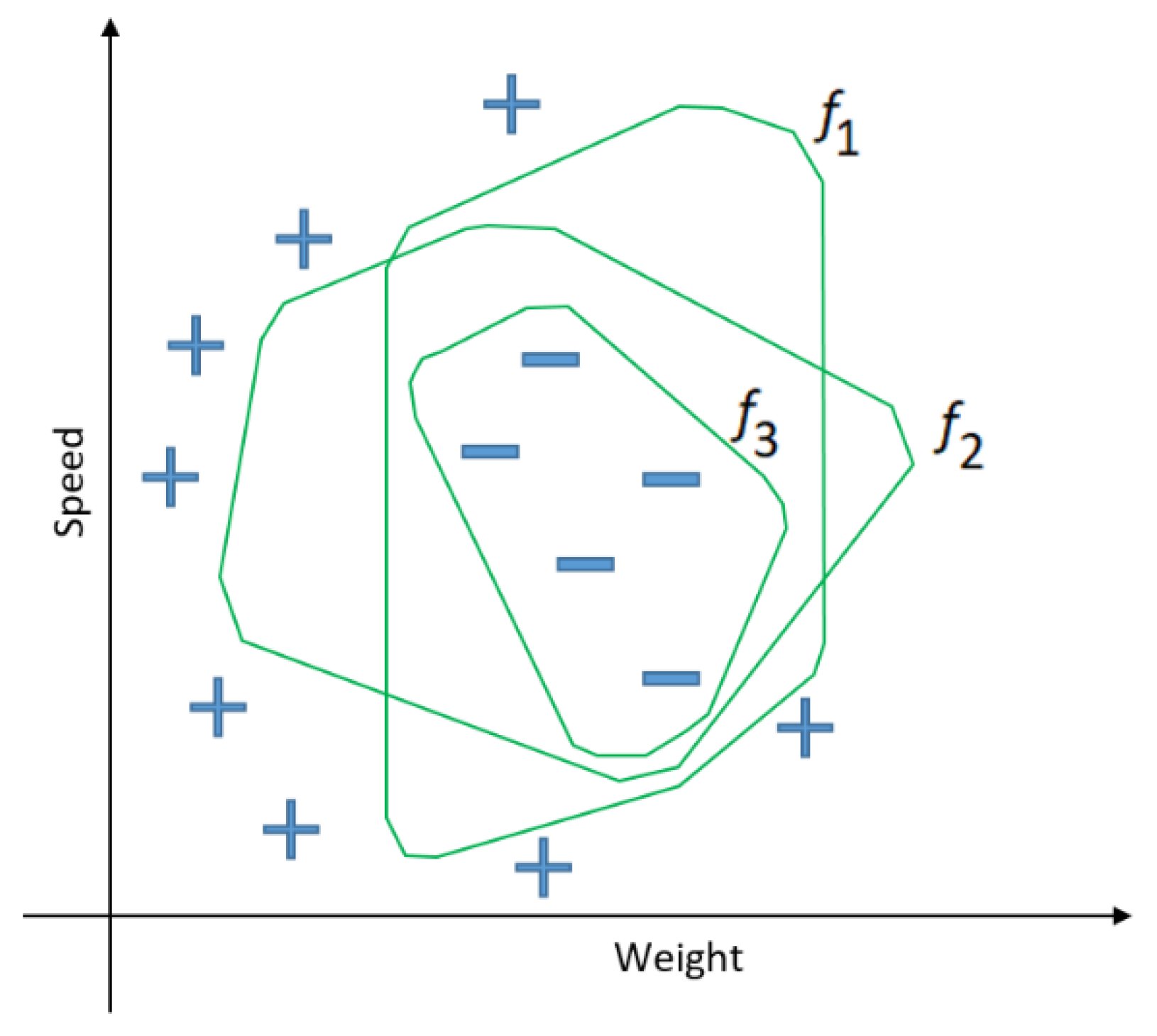
- Bagging – The high variance of available data in a dataset affects the low generalization power of the model, even if the training dataset is enlarged. Research shows that the solution to this problem lies in the Bagging method, which combines Bootstrapping and Aggregating methods [45]. Bootstrapping focuses on reducing the classifier variance and decreasing overfitting by resampling the data from the training set [45]. By using n training subsets, n training results are obtained, and the final classification results are derived using aggregation strategies such as averaging or voting [37].
- Boosting Bagging - Stacking. The main idea of this learning paradigm is that models are sequentially added to the ensemble, with each iteration requiring the new model to specifically process the data on which its predecessors or weak learners made errors [45]. The main goal of the Boosting paradigm is to reduce Bias, i.e., systematic error caused by the model itself, rather than its sensitivity to data variations. In the boosting approach, weights are implicitly assigned to models based on their performance, similar to the concept of a weighted average ensemble. Popular variants of this approach featured in research include Adaptive Boosting (AdaBoost), Gradient Boosting and Extreme Gradient Boosting (XGBoost).
- Stacking. Bagging and Boosting methods typically use homogeneous weak learners or models as ensemble members. Stacking often works with heterogeneous weak learners that learn in parallel, and their results are combined by training a meta-learner for final output classification. This means that the target learner uses model classifications as input variables [37,45]. In ensemble averaging, such as Random Forest, classifications from multiple models are combined, with each model contributing equally regardless of performance. In contrast, a weighted average ensemble measures the contribution of each member based on classification performance, thereby offering an improvement over ensemble averaging.
5.5. Discussion
- The classifications of the first input vector from all individual models are fed to the input of the Combiner;
- If CHAID and C5.0 provide classifications, the final classification is equal to that value. If there are discrepancies between the classifications of these two models, the final classification of the input is determined by a voting method. This implies that a certain category must have a majority of votes from the six created models. For all other situations, the result of the CHAID model is taken as the final classification.
- If final classifications are not determined for all input vectors, the next input vector is fed to the input of the Combiner and the process returns to step 2;
- If final classifications are determined for the entire test dataset, the algorithm terminates.
6. Conclusions
Author Contributions
Funding
Institutional Review Board Statement
Informed Consent Statement
Data Availability Statement
Conflicts of Interest
References
- Riste, R.; Slobodan, O.; Zlatko, Z.; Vasko, G.; Ivona, N.; Vlatka, K. Road safety inspection in the function of determining unsafe road locations. The 9th International Conference “CIVIL ENGINEERING – SCIENCE AND PRACTICE”, Kolašin, Montenegro, 5-9 March 2024.
- Banjanin, M.K.; Bjelošević, R.; Vasiljević, M.; Stojčić, M.; Đukić, A. The Method of the Research Loop of Teletraffic in the Structure of the System of Public Urban Passenger Transport. In Proceedings of the XIX International Symposium New Horizons 2023 of Transport and Communication; Saobraćajni fakultet Doboj, Univerzitet u Istočnom Sarajevu: Doboj, Bosnia and Herzegovina, 24-25 November 2023. (pp.4-15).
- Miller, T. Explanation in artificial intelligence: Insights from the social sciences. Artificial Intelligence 2019, 267, 1–38. [CrossRef]
- Pentland, B.T.; Liu, P.; Kremser, W.; Haerem, T. The dynamics of drift in digitized processes. MIS Quarterly 2020, 44(1), 19–47. [CrossRef]
- Iversen, V.B. Teletraffic engineering and network planning; dtu Fotonik: Copenhagen, Denmark, 2015.
- Banjanin, K.M.; Gojković, P. Analitičke Procedure u Inženjerskim Disciplinama; Saobraćajni fakultet: Doboj, Bosnia and Herzegovina, 2008.
- Pitt, J.; Mamdani, A. A Protocol-Based Semantics for an Agent Communication Language. In Proceedings of the Sixteenth International Joint Conference on Artificial Intelligence (IJCAI-99), Stockholm, Sweden, 2–6 August 1999; Volume 99, pp. 486-491.
- Alli, V. The Future of Knowledge: Increasing Prosperity through Value Networks; Butterworth-Heinemann: Amsterdam, The Netherlands, 2003. ISBN 0750675918.
- Polanyi, K. For a New West: Essays, 1919–1958; Polity Press: Cambridge, UK, 2014. ISBN-13: 978-0-7456-8443-7.
- Davenport, T.H.; Prusak, L. Working knowledge: How organizations manage what they know; Harvard Business School Press: Boston, MA, USA, 2000; pp. 1-7.
- Barna-Lipkovski, M. Konstruisanje Ličnog Identiteta Jezikom i Hronotopom Interneta: Umetničko Delo Scenskog Dizajna. Ph.D. Thesis, University of Novi Sad, Novi Sad, Serbia, 2021. Available online: https://nardus.mpn.gov.rs/handle/123456789/20928?show=full (accessed on 3 September 2024).
- Hicks, B.J.; Culley, S.J.; Allen, R.D.; Mullineux, G. A framework for the requirements of capturing, storing and reusing information and knowledge in engineering design. International Journal of Information Management 2002, 22(4), 263-280. [CrossRef]
- Hackos, J.T.; Hammar, M.; Elser, A. Customer partnering: data gathering for complex on-line documentation. IEEE Transactions on Professional Communication 1997, 40(2), 83-96. [CrossRef]
- King, W.R.; Teo, T.S.H. Key Dimensions of Facilitators and Inhibitors for the Strategic Use of Information Technology. Journal of Management 1996, 1(1), 1-25. http://www.jstor.org/stable/40398177.
- Watson, H.J.; Houdeshel, G.; Rainer, R.K. Jr. Building executive information systems and other decision support applications, 1st ed.; Wiley: Hoboken, New Jersey, United States, 1996.
- Byun, D.H.; Suh, E.H. A methodology for evaluating EIS software packages. Journal of Organizational Computing and Electronic Commerce 1996, 6(3), 195-211. [CrossRef]
- Simon, H.A. Administrative Decision Making; Carnegie Institute of Technology: Pittsburgh, PA, USA, 1996.
- Kahneman, D. Maps of Bounded Rationality: Psychology for Behavioral Economics. The American Economic Review 2003, 93(5), 1449-1475. [CrossRef]
- Benyon, D.; Murray, D. Adaptive systems: From intelligent tutoring to autonomous agents. Knowledge-Based Systems 1993, 6(4), 197-219. [CrossRef]
- Cilliers, P. Complexity and Postmodernism; Routledge: New York, NY, USA, 1998.
- Banjanin, M. Komunikacioni Inženjering; Saobraćajno tehnički fakultet: Doboj, Bosnia and Herzegovina, 2006.
- Addy, R. Effective IT Service Management – To ITIL and Beyond; Springer: New York, NY, USA, 2007.
- Banjanin, M.; Petrović, L.; Tanackov, I. Multiagent Communication Systems. In Proceedings of the XIV Međunarodna naučna konferencija Industrijski sistemi IS'08, Novi Sad, Serbia, 2-3 October 2008.
- Banjanin, M.K. Dinamika komunikacija-interkulturni poslovni kontekst; Megatrend Univerzitet primenjenih nauka: Beograd, Serbia, 2003. ISBN 86-7747-106-5.
- Michalski, R.S.; Bratko, I.; Kubat, M. Machine Learning and Data Mining, Methods and Applications; John Wiley & Sons: West Sussex, UK, 1998.
- Kurbel, K.E. The Making of Information Systems Software Engineering and Management in a Globalized World; Springer-Verlag: Berlin, Germany, 2008. [CrossRef]
- Popovic, D. Model unapređenja kvaliteta procesa životnog osiguranja. Ph.D. Thesis, University of Novi Sad, Novi Sad, Serbia, 2020. Available online: https://nardus.mpn.gov.rs/handle/123456789/10399 (Accessed on 3 September 2024).
- Banjanin, M.K.; Đukić, A.; Stojčić, M.; Vasiljević, M. Machine Learning Models in the Classification and Evaluation of Traffic Inspection Jobs in Road Traffic and Transport. In Proceedings of the 13th International Scientific Conference SED 2023, Vrnjačka Banja, Serbia, 5-8 June 2023.
- Tang, J.; Zhang, D.; Sun, X.; Qin, H. Improving Temporal Event Scheduling through STEP Perpetual Learning. Sustainability 2022, 14(23), 16178. [CrossRef]
- Fourez, T.; Verstaevel, N.; Migeon, F.; Schettini, F.; Amblard, F. An Ensemble Multi-Agent System for Non-Linear Classification. arXiv preprint 2022, arXiv:2209.06824. [CrossRef]
- Zhou, J.; Asteris, P.G.; Armaghani, D.J.; Pham, B.T. Prediction of Ground Vibration Induced by Blasting Operations through the Use of the Bayesian Network and Random Forest Models. Soil Dynamics and Earthquake Engineering 2020, 139, 106390. [CrossRef]
- Andjelković, D.; Antić, B.; Lipovac, K.; Tanackov, I. Identification of hotspots on roads using continual variance analysis. Transport 2018, 33(2), pp. 478–488. [CrossRef]
- Holdaway, M.; Rauch, M.; Flink, L. Excellent Adaptations: Managing Projects through Changing Technologies, Teams, and Clients. In Proceedings of the 2009 IEEE International Professional Communication Conference, Waikiki, HI, USA, 19-22 July 2009.
- Brown, S. M.; Santos, E.; Banks, S. B. Utility theory-based user models for intelligent interface agents. In Advances in Artificial Intelligence: 12th Biennial Conference of the Canadian Society for Computational Studies of Intelligence, AI'98 Vancouver, BC, Canada, June 18–20, 1998 Proceedings 12 (pp. 378-392). Springer Berlin Heidelberg. [CrossRef]
- Milanović, M.; Stamenković, M. CHAID Decision Tree: Methodological Frame and Application. Economic Themes 2016, 54(4), 563-586. [CrossRef]
- Potdar, K.; Pardawala, T.S.; Pai, C.D. A Comparative Study of Categorical Variable Encoding Techniques for Neural Network Classifiers. International Journal of Computer Applications 2017, 175(4), 7-9. [CrossRef]
- Wu, X.; Wang, J. Application of Bagging, Boosting and Stacking Ensemble and Easy Ensemble Methods to Landslide Susceptibility Mapping in the Three Gorges Reservoir Area of China. International Journal of Environmental Research and Public Health 2023, 20(6), 1-31. [CrossRef]
- Banjanin, M.K.; Stojčić, M.; Danilović, D.; Ćurguz, Z.; Vasiljević, M.; Puzić, G. Classification and Prediction of Sustainable Quality of Experience of Telecommunication Service Users Using Machine Learning Models. Sustainability 2022, 14(24), 17053. [CrossRef]
- Chorianopoulos, A. Effective CRM Using Predictive Analytics; Wiley: West Sussex, UK, 2015. ISBN: 978-1-119-01155-2.
- Saatçioğlu, Ö.Y. Üniversite Yönetiminde Etkinliğin Arttırılmasına Yönelik Bilgi Sistemlerinin Tasarlanması ve Uygulanması. Ph.D. Thesis, Dokuz Eylul University, Izmir, Turkey, 2024. Available online: https://avesis.deu.edu.tr/yasar.saatci/indir?languageCode=en (accessed on 3 September 2024).
- Scikit-learn. Available online: https://scikit-learn.org/stable/auto_examples/svm/plot_rbf_parameters.html (accessed on 8 November 2022).
- Laplace, P.S. A Philosophical Essay on Probabilities; Truscott, F.W., Emory, F.L., Translators; Dover Publications: New York, NY, USA, 1951.
- Neskovic, S.; Petkovic, A. The Methodology of Analysis and Assessment of Risk for Corruption in the Company Operations. Vojno Delo 2016. [CrossRef]
- IBM. https://www.ibm.com/docs/en/spss-modeler/18.5.0?topic=nodes-chaid-node (accessed on 5 July 2024).
- Twiki. Available online: https://twiki.di.uniroma1.it/pub/ApprAuto/WebHome/8.ensembles.pdf (accessed on 7 July 2024).
- IBM SPSS Modeler-help. Available online: http://127.0.0.1:50192/help/index.jsp?topic=/com.ibm.spss.modeler.help/clementine/trees_quest_fields.htm (accessed on 7 July 2024).
- IBM SPSS Modeler-help. Available online: http://127.0.0.1:55706/help/index.jsp?topic=/com.ibm.spss.modeler.help/clementine/c50_modeltab.htm (accessed on 7 July 2024).
- IBM SPSS Modeler-help. Available online: http://127.0.0.1:56089/help/index.jsp?topic=/com.ibm.spss.modeler.help/clementine/rf_fields.htm (accesed on 6 July 2024).
- IBM SPSS Modeler-help. Available online: http://127.0.0.1:57164/help/index.jsp?topic=/com.ibm.spss.modeler.help/clementine/model_nugget_variableimportance.htm (accessed on 6 July 2024).
- Klu. Available online: https://klu.ai/glossary/accuracy-precision-recall-f1 (accessed on 3 September 2024). (accessed on 3 September 2024).
- Knezevic, I. Analiza dinamičkog ponašanja kugličnih ležaja primenom veštačkih neuronskih mreža. Ph.D. Thesis, University of Novi Sad, Novi Sad, Serbia, 2021. Available online: https://nardus.mpn.gov.rs/handle/123456789/17986 (accessed on 3 September 2024).
- Petronijevic, M. Uticaj oksidacionih procesa na bazi ozona, vodonik-peroksida i UV zračenja na sadržaj i reaktivnost prirodnih organskih materija u vodi. Ph.D. Thesis, University of Novi Sad, Novi Sad, Serbia, 2020. Available online: https://nardus.mpn.gov.rs/handle/123456789/11378 (accessed on 3 September 2024).
- Kuhn, M.; Johnson, K. Applied Predictive Modeling; Springer: New York, NY, USA, 2013. [CrossRef]
- IBM SPSS Modeler-help. Available online: http://127.0.0.1:62164/help/index.jsp?topic=/com.ibm.spss.modeler.help/clementine/c50_modeltab.htm (accesed on 6 July 2024).
- Sarker, I.H. Machine Learning: Algorithms, Real-World Applications and Research Directions. SN Computer Science 2021, 2(3), 160. [CrossRef]
- Ndung'u, R.N. Data Preparation for Machine Learning Modelling. International Journal of Computer Applications Technology and Research 2022, 11(6), 231-235. [CrossRef]
- Xu, H.; Zhou, J.; Asteris, P.G.; Armaghani, D.J.; Tahir, M.M. Supervised Machine Learning Techniques to the Prediction of Tunnel Boring Machine Penetration Rate. Applied Sciences 2019. [CrossRef]
- Russell, S.J.; Norvig, P. Artificial Intelligence: A Modern Approach; 4th ed.; Pearson: New York, NY, USA, 2021.
- Goodfellow, I.; Bengio, Y.; Courville, A. Deep Learning; MIT Press: Cambridge, MA, USA, 2016.
- Mitchell, T.M. Machine Learning; McGraw-Hill: New York, NY, USA, 1997.
- Molar, C. Kulturni Inženjering; Clio: Beograd, Serbia, 2000.
- Škorić, M. The Standard Model of Social Science and Recent Attempts to Integrate Sociology, Anthropology and Biology. Ph.D. Thesis, Filozofski Fakultet Univerziteta u Novom Sadu, Novi Sad, Serbia, 2010.
- Zelenović, D. Intelligent Business; Prometej: Novi Sad, Serbia, 2011.

| Activity | Location | Host | Object | Event type | Periodicity | Event Significance |
||
|---|---|---|---|---|---|---|---|---|
| Activity | Correlation Coefficient | 1.000 | -.002 | .016 | .208** | -.015 | -.086** | -.222** |
| Sig. (2-tailed) | . | .862 | .100 | .000 | .116 | .000 | .000 | |
| Location | Correlation Coefficient | -.002 | 1.000 | -.133** | -.007 | -.059** | .034** | .005 |
| Sig. (2-tailed) | .862 | . | .000 | .439 | .000 | .000 | .579 | |
| Host | Correlation Coefficient | .016 | -.133** | 1.000 | .278** | -.221** | .135** | .158** |
| Sig. (2-tailed) | .100 | .000 | . | .000 | .000 | .000 | .000 | |
| Object | Correlation Coefficient | .208** | -.007 | .278** | 1.000 | -.112** | -.046** | -.074** |
| Sig. (2-tailed) | .000 | .439 | .000 | . | .000 | .000 | .000 | |
| Event type | Correlation Coefficient | -.015 | -.059** | -.221** | -.112** | 1.000 | -.302** | -.226** |
| Sig. (2-tailed) | .116 | .000 | .000 | .000 | . | .000 | .000 | |
| Periodicity | Correlation Coefficient | -.086** | .034** | .135** | -.046** | -.302** | 1.000 | .160** |
| Sig. (2-tailed) | .000 | .000 | .000 | .000 | .000 | . | .000 | |
| Event Significance | Correlation Coefficient | -.222** | .005 | .158** | -.074** | -.226** | .160** | 1.000 |
| Sig. (2-tailed) | .000 | .579 | .000 | .000 | .000 | .000 | . | |
| Model | Accuracy | Method | Predictors | Model Size (Synapses) | Records |
|---|---|---|---|---|---|
| 1 | 92.7% | MLP | 5 | 7418 | 9,906 |
| 2 | 63.7% | MLP | 5 | 4439 | 9,906 |
| 3 | 68.6% | MLP | 5 | 3569 | 9,906 |
| 4 | 60.4% | MLP | 5 | 2853 | 9,906 |
| 5 | 37.5% | MLP | 5 | 2116 | 9,906 |
| Observed categories | Classification by model | Percent correct | |||||||
|---|---|---|---|---|---|---|---|---|---|
| 1 | 2 | 3 | 4 | 5 | 6 | 7 | 8 | ||
| 1 | 2 | 0 | 0 | 2 | 0 | 0 | 0 | 0 | 50 |
| 2 | 0 | 1 | 0 | 9 | 1 | 0 | 0 | 1 | 8 |
| 3 | 0 | 0 | 2 | 1 | 0 | 0 | 1 | 0 | 50 |
| 4 | 0 | 1 | 0 | 269 | 14 | 3 | 4 | 0 | 92 |
| 5 | 0 | 1 | 1 | 16 | 79 | 4 | 2 | 0 | 77 |
| 6 | 0 | 1 | 2 | 18 | 4 | 17 | 0 | 1 | 40 |
| 7 | 0 | 1 | 1 | 7 | 3 | 1 | 14 | 2 | 48 |
| 8 | 0 | 1 | 1 | 1 | 1 | 2 | 0 | 4 | 40 |
| Percent correct | 1 | 17 | 29 | 83 | 77 | 63 | 67 | 50 | 78 |
| Model | Hyperparameters |
|---|---|
| CHAID | Maximum Tree Depth: 5; Minimum records in parent branch – 2% of the total dataset; Minimum records in child branch – 1% of the total dataset; Significance level for splitting = 0.05; Significance level for merging = 0.05; Minimum Change in Expected Cell Frequencies: 0.001; Maximum Iterations for Convergence: 100; Maximum surrogates: 5. |
| C&R Tree | Maximum Tree Depth: 5; Minimum records in parent branch – 2% of the total dataset; Minimum records in child branch – 1% of the total dataset; Minimal impurity change (Gini Index): 0.0001. |
| QUEST | Maximum Tree Depth: 5; Maximum surrogates: 5; Minimum records in parent branch – 2% of the total dataset; Minimum records in child branch – 1% of the total dataset; Significance level for splitting = 0.05. |
| C5.0 | Mode: Simple; Favor: Accuracy |
| Random Trees | Number of models to build: 100; Maximum number of nodes: 10000; Maximum tree depth: 10; Minimum child node size: 5. |
| SVM | Stopping criteria: 10-3; Regularization parameter (C): 10; Kernel type: RBF; RBF Gamma: 0,1; |
| Observed classes | Classification by model ensemble | Precision | Recall | F1 score | |||||
|---|---|---|---|---|---|---|---|---|---|
| 2 | 3 | 4 | 5 | 6 | 7 | ||||
| 2 | 0 | 0 | 1 | 0 | 0 | 0 | - | 0 | - |
| 3 | 0 | 0 | 1 | 0 | 0 | 0 | - | 0 | - |
| 4 | 0 | 0 | 43 | 0 | 1 | 0 | 0.9348 | 0.9773 | 0.9555 |
| 5 | 0 | 0 | 1 | 9 | 1 | 0 | 1 | 0.8181 | 0.8999 |
| 6 | 0 | 0 | 0 | 0 | 2 | 0 | 0.5 | 1 | 0.6667 |
| 7 | 0 | 0 | 0 | 0 | 0 | 5 | 1 | 1 | 1 |
Disclaimer/Publisher’s Note: The statements, opinions and data contained in all publications are solely those of the individual author(s) and contributor(s) and not of MDPI and/or the editor(s). MDPI and/or the editor(s) disclaim responsibility for any injury to people or property resulting from any ideas, methods, instructions or products referred to in the content. |
© 2024 by the authors. Licensee MDPI, Basel, Switzerland. This article is an open access article distributed under the terms and conditions of the Creative Commons Attribution (CC BY) license (http://creativecommons.org/licenses/by/4.0/).


