
Submitted:
06 September 2024
Posted:
09 September 2024
You are already at the latest version
Abstract
Efforts to optimize the design and enhance the efficiency of standing-wave thermoacoustic refrigerators (SWTAR), particularly those with parallel plate stacks, are crucial for achieving rapid and straightforward engineering estimates. This study primarily focuses on optimizing the Coefficient of Performance (COP) by combining the linear thermoacoustic theory (LTT) with the Design of Experiments (DOE) approach. The investigation centers around five key parameters affecting the COP, once the working gas is selected. Then, based on the LLT theory, the COP was estimated numerically, over defined intervals of those five parameters. Moreover, through quantitative and qualitative effect analyses, these five parameters and their interactions are determined. Utilizing a transfer function and surface response analyses based on the COP, the study aims to delineate the best COP value as well as the contribution of the thermoacoustic parameters and their interactions. Furthermore, a comparison between contour and surface responses and several statistical decision approaches applying the Full Factorial Design verify the robustness of the study’s findings. Ultimately, the COP results obtained align with existing literature, underscoring the validity and relevance of the study’s methodologies and conclusions.
Keywords:
Thermoacoustics
; Design of experiments
; Linear Thermoacoustic Theory
; Pearson Analysis
; ANOVA
; Transfer Function
1. Introduction
Thermoacoustic refrigerators are devices, that use sound waves to generate cooling without moving parts. Due to the complex relationship between the multiple variables that determine its performance, optimization studies are required from a practical point of view. Many proposals are currently being explored to optimize thermoacoustic refrigerators, not only the performance response to environmental concerns related to many refrigerants but also to obtain fast and simple engineering estimates. The performance response depends primarily on the system’s design parameters, including operating conditions, the structural geometry of stack/regenerator, thermo-physical properties of the stack, working fluid, and acoustic driver. These design parameters can be studied and optimized from different perspectives and study groups/areas such as:
- Materials and structural design: Optimizing the materials of the acoustic resonator and internal components can enhance the durability and efficiency of the thermoacoustic cooler. This involves studies on composite materials, aerogels [17], thermal conductivity, mechanical resistance, and durability under operating conditions [12]–[14].
- Acoustics and vibrations: Since thermoacoustic refrigerators use sound waves to generate pressure changes and thus cooling, they can be studied from the perspective of acoustics and vibrations. This includes optimizing acoustic resonator geometry and system design to maximize acoustic-to-thermal energy transfer efficiency [9,10,15,16,20].
- Control and electronics: Electronic control of the thermoacoustic cycle can be crucial to optimize the stability and performance of the refrigerator. Control algorithms, temperature and pressure sensors, and the integration of electronic components can be studied to improve system accuracy and efficiency. [18]
In the literature, the efficiency of a thermoacoustic device is given by the Coefficient of Performance () [1,17] defined as the ratio between heat flow () and the acoustic work (W) on the stack. From an energy efficiency optimization perspective, the generated in the stack must be maximized. Regarding geometrical optimization parameters, several studies have been carried out, including intelligent optimization techniques such as Genetic Algorithms [1,7] Response Surface methodology (RSM) [15,16], Nonlinear programming models with discontinuous derivatives (DNLPs) [6], among others. Most of these works have been based on the linear thermoacoustic theory [9]-[10]. Using dimensionless analysis and short stack and boundary layer approximations, Tijani [9] obtained dimensionless expressions for and W; which depend on eight dimensionless parameters. Despite these simplifications, to the authors’ knowledge, no study has yet been carried out to identify and quantify the contribution of each of these parameters, as well as the cross-effect of their interactions. When the working gas is chosen, the depends on five parameters, namely D, B, , , , see Figure 1.
In this work we present results from the application of the design of experiments (DOE) [21] using MINITAB [22], to quantitatively and qualitatively estimate the individual contribution of the five parameters described above to the and their interactions. This study builds upon the methodology outlined by Tijani [9], readers interested in a detailed development of the theory are encouraged to refer to this work.
2. Methods
2.1. COP Estimation for Thermoacoustic Devices
The is a measure of the efficiency of a refrigeration system, heat pump, or heat engine. In the context of the efficiency of transferring acoustic energy from the speaker to the environment, the and acoustic power are related [9]-[10].
The performance of a thermoacoustic system depends strongly on the characteristics and properties of the porous medium (referred to in the Literature as the stack) used to exchange heat with the working fluid, see Figure 1.
For the development of a thermoacoustic refrigerator, the basic theory and equations for linear standing-wave thermoacoustic systems have been extensively developed by Tijani [9]-[10]. The term “regenerator” is used when the pore size of the porous element is small compared to the depth of thermal penetration. The thermal penetration depth refers to the layer around the regenerator where the thermoacoustic phenomenon occurs.
The thermal and viscous penetration depths are defined as follows:
and
Where:
- is the angular frequency of the sound wave, is the design frequency.
- , K and are the viscosity, density, thermal conductivity, and isobaric specific heat of the gas respectively.
Thus, the performance of the thermoacoustic regenerator depends on many parameters. Olson and Swift [19] proposed the application of Similitude in thermoacoustics without using the acoustic approximation.
The dimensionless cooling power obtained from similitude and the acoustic power , where is the mean pressure; a is the sound velocity, and A is the cross-sectional area of the stack proposed by [19] are mentioned by Tijani et al. [10] that rewrites and in dimensionless form by using dimensionless parameters as:The equations which are important to thermoacoustics (continuity, motion, and heat transfer) are rewritten in dimensionless form, verifying that the list of dimensionless variables obtained from similitude is complete.
Where , is the dimensionless thermal penetration depth, is the regenerator blocking ratio, is half the distance between the stack plates and l is half the thickness of the regenerator planes, is the dimensionless temperature difference, k is the wave number, is the dimensionless stack position, is the dimensionless stack length, is the ratio of isobaric to isochoric specific heats, is the dimensionless viscous penetration depth, and D is the drive ratio.
Thus, the performance of the regenerator depends explicit on dimensionless variables, as shown in Equations (3) and (4). It is important to note that the Prandtl number is proportional to the ratio of the thermal and viscous penetration depths, see Equations (1) and (2) respectively. By other hand, the dimensionless viscous penetration depth is implicit in the calculation even though, it is not present in Equations (3) and (4). The Prandtl number is an essential parameter for understanding and analyzing the convective heat transfer characteristics of fluids. If gas working is chosen, then the depends on five dimensionless parameters. For the analysis in this study, five of these dimensionless variables are selected from Table 1: drive ratio D, the blocking ratio B, the dimensionless temperature difference , the dimensionelss stack position , the dimensionless stack length . The analysis focuses on these variables through the defined as . Our analysis considers a quarter-wavelength resonator using air as a working gas.
2.2. Design of Experiments (DOE)
The Design of Experiments (DOE) or factorial design, is a regression analysis extensively employed in industry to identify and control critical parameters for enhancing product quality [21]. Experimental studies are normally time-consuming, and requiere examining the effects of two or more factors. Factorial design allows for the investigation of all possible combinations of the levels of specified factors (see Figure 2). Due to the time and expensive of the experiments, the selection of the factors to be analyzed must be made with careful consideration. One of the main reasons to apply a DOE is to minimize the number of experimental trials and to derive a transfer function. Another benefit of using DOE is the seamless integration of experimental data with numerical methods, such as the finite element method (FEM) to simulate alterations in physical parameters (factors).
A complete factorial design incorporates all possible "levels" of a given number of "factors". These levels are categorized as "low" (in red) and "high" (in blue) and are represented by the symbols "-" and "+", respectively (see Figure 2). The effect of a factor is defined as the change in the response cause by altering the level of that factor. This is referred to as the main effect1 because it represents the primary influence in the experiment. Furthermore, the difference in response in some experiments between levels of one factor may vary across the levels of the other factors. When this variation occurs, it indicates an interaction between the factors. Analyzing the main effects and interactions between factors in the results the archivement of one or more of the following objectives:
- Determine the optimal condition within a specified range.
- Assess the contribution of individual factors and their interactions.
- Predict the response under optimal conditions.
The estimation of the contribution of each factors and their interactions will be determined within a specified range or limit.
In this study, the parameter range is set to derive a response function () which is defined by the parameters or factors (), coefficients () and the error term (), see Equations (5)–(7):
where:
The response of the will be represented by , where is an matrix of independent variables (defined as A,B,C,D, and E in Table 2. The vector b contains the regression coefficients and is a vector of random errors. The system’s will be calculated in the following section using the dimensionless parameters, expressed in Equations (3) and (4).
Additionally, once the parameters are established, the DOE is primarily analyzed in three stages, encompassing all the theorical calculation. These stages are:
- Planning stage
- Analysis stage
- Results stage
The most crucial part of the DOE is the planning stage. It is vital the development of an orthogonal matrix to account for the effects of various factors influencing the response. According the literature, the relationship of these factors depends on the physical parameters of the thermoacoustic refrigerator, as detailed in Table 2. These factors will be analyzed quantitatively and qualitatively in the DOE.
Therefore, five parameters, each with two levels (low and high), are put forward as factors to create a full factorial. Table 3 illustrates the matrix to be followed based on the levels by factors of Table 2. The determination of the interaction signs is calculated by multiplying the signs of each interaction shown in Table 3 up to the third interaction for matrix size ratios. For example, the first value in column AB is ”+” derived by multiplying the signs and . For the higher interactions, the remaining signs are calculated similarly. Using these interaction signs and the response, the average values (low and high) are computed to obtain the coefficients. These coefficients are calculated with MINITAB 19 [22] and used to generate the main interaction effects plots. It is crucial that the low and high levels remain orthogonal to each other, preserving the same proportion between the factors. These values depend on the nominal values chosen for the DOE. For intance, if the nominal value of a factor is 0.10, the low and high limits will be 0.05 and 0.15, respectively.
Several statistical decision approaches constitute the analysis phase: examining the significance of the distribution, performing analysis of variance (ANOVA), and evaluating the R-Sq coefficient (which represents the ratio of the variation explained by each variable). These methods enable the identification of significant coefficients and facilitate the contruction of the transfer function in two stages.
First, the significance of the distribution is assessed to establish a confidence level of 95%, which corresponds to a significance level of =0.05 for a single proportion of population. The Alpha () represents the maximum acceptable probability of incorrectly rejecting the null hypothesis when the alternative hypothesis is true. The results are evaluated using average analysis2, the standard deviation3 the sum of squares deviations and the variance of the factors affecting the , where N represents the number of runs and "DF" stands for degrees of freedom.
Second, the ANOVA test evaluates the averages that affect the to identify the variance among factors and their interactions. A P-value ≤ 0.05 indicates the significance of the main parameters and their interactions in the ANOVA analysis. Coefficients and errors are determined through on statistical decision approximations using the Anderson-Darling Test method with MINITAB 19, that assess the significance and normality of the data distribution [22]. As shown in Table 3, the ANOVA is conducted using the responses derived from the orthogonal matrix,. Numerous visualizations, such as main effects plots, interaction effects plots, Pareto charts, cube plots, contour plots, and surface plots, are utilized to analyze the factors and interactions affecting the .
Finally, the results phase entails constructing the transfer function using the coefficients derived from the R-Sq value. The relationship between the variation of each variable and the total variation (variation of the Mean Sum of Squares (MSS)) is quantified with the coefficient of determination R-Sq. The R-Sq is also referred to as a measure of the goodness of fit. A highher R-Sq value, approaching 100 %, suggests a better representation of the total variation of the response.
3. Results
The parameters intervals for the ’s are defined, as shown in Table 4. The ’s values for each trial are computed using a numerical rutine in Python 3.6 [23] based on the Equations (3 and 4 for each established interval, see Table 5. A representative plot of the is observed in Figure 3 as a function of and defined in Table 1. Typically, the increases as the dimensionless stack position is decreased. Based on the maximum ’s values obtained numerically, the DOE analysis is carried in three steps:
- Establish the orthogonal design to determine the of a thermoacoustic cooling system, as outlined by Tijani [10].
- Perform Pearson analysis: Assess main and interactions effects, Pareto chart, cube plots, contours, and surfaces plots.
- Conduct ANOVA analysis and develop transfer function.
3.1. COP’s Orthogonal Array
The full factorial design, is created by generating a set of combinations based on the number of parameters and their specified values.
Table 4 provides the values for the lower and upper limits. Table 5 presents the matrix of = 32 runs plus the center point, along with the values obtained for each combination. The order of runs is randomized to prevent aliasing4. The response is calculated for each combination of "low" and "high" values of the parameters.
The DOE is conducted using each combination to determine the response. The subsequent step involves analyzing the main effects and interactions of the parameters affecting the . Note that Table 5 includes 33 runs due to the inclusion of a central point to assess curvature. This central point marked in red, is shown in Figures, Figure 4 and Figure 5. If the central point deviates significantly from the line that joins the means of the vertex points, it indicates a potential curvature in the relationship, and its P-value will be assessed for statistical significance. If the contribution of curvature is found to be insignificant, it implies that the variation in response with the chosen factors does not exhibit substantial changes.
3.2. Pearson Analysis
A main effects analysis can be conducted to identify the critical parameters and interactions using a Pearson correlation5, back when the values are obtained based on the combinations in Table 5. Pearson correlation assesses the linear relationship between defined variables for a given significance level (in this case =0.05).
Moreover, interactions between parameters can also be assessed. It is crucial to understand that the range of values was established by multiplying each of the parameters at the central point of Table 5 (run 33) by a value of 0.5, and then adding and subtracting this result from the center point to define the upper and lower limits, respectively.
Multiplying the factors by this value to adjust for the lower and upper limits is referred to as orthogonality in the full factorial design, which helps to maintain the "balance" of the DOE. The effects of each chosen parameter on the are depicted in Figure 4. Main effects are determined by the slope of the values obtained between the defined limits for each parameter: a steeper slope indicates a stronger effect of the parameter. According to the plot results, the dimension parameters with the most significant impact on the are: the temperature difference , the length of the regenerator , the Blocking ratio B as well as it’s position . Counterintuitively, the parameter D does not have a notable effect on the . However a comprehensive quotient analysis of Equations (3) and (4) reveals that this outcome is anticipated. As shown in the main effect results for in Figure 4 , parameter D does not affect the .
Additionally, Figure 5 illustrates the interactions between parameters. These interactions are identified based on the slope observed between the specified limits. The columns in the interaction graph represent the response for a specific interaction of a given factor (- or +), while the rows represent the average response for a particular configuration (- or +) of factor interactions (columns), as shown in Figure 5. Parallel lines in the interactions suggest no interaction effect, whereas a larger difference in slope between the lines indicates a stronger interaction effect. Consequently, the ”low” values within the defined range show a positive effect on results compared to the ”high” values. The interactions with the most significant influence, depicted in Figure 5, are between the following parametes pairs in the lower section: *B, *, *B. These interactions, especially those in the lower section of the graph, positively impact the average value due to their interaction slopes. Only the pair * in the upper section also shows a positive effect on improving the average value.
The positive effect on both the upper and lower limits of the interaction between *B factors is emphasized. However, the interaction graph alone does not reveal the statistical interaction significance of these interactions. To further understand the impact of main and interaction effects, a Pareto6 chart can be used. A Pareto chart helps identify which factors have the most significant influence on the response. It shows the absolute values of the standardized effects from the largest to the smallest. Standardized effects are t-statistics used to test the null hypothesis that the effect is zero [22]. The reference or threshold line for statistical significance depends on the significance level (denoted by ). Unless a stepwise selection method is used to define an alpha value, the significance level is calculated as 1 minus the confidence level for the analysis. The reference line indicates which effects are statistically significant. Factors such as , , the interaction *B and the others with bars extending above the threshold red dashed line (value of 12.7), see Figure 6, are typically the main contributors to be focused on the subsequent Analysis of variance (ANOVA) subsection. With the current model terms, these factors are statistically significant at the 0.05 level.
Additionally, the cube plot, contour plots and surface plots will offer a visual representation of the trends of each interaction based on the established intervals. A cube plot (see Figure 7) illustrates the relationships among the five factors and their impact on the response measure for 2-level factorial designs or Plackett-Burman designs. This plot visually represents the factorial design, showing how different factors affect the values. By examining the cube plot, one can observe the most significant impacts on the values at the lower limits of the factors.
Contour plots and surfaces are used to visualize and explore the potential interaction among all parameters relative to the response. Contour plots provide a two-dimensional view of the lower and upper limits, with the x and y axes representing these limits, while the contours indicates the response. Similar to a topographic map, where longitude, latitude, and elevation are plotted and connected by contour lines, the contour plot displays x, y, and z values connected by lines of constant response. In the contour plots, a maximum response of 1.76 can be observed in the products for the lower limits, such as , , , and , as shown in Figure 8 and Figure 9. Notably, at the center point in Figure 8, the maximum value is 1.4, specifically for the product .
The surface plots, illustrated in Figs. Figure 10 and Figure 11, display the variable response surfaces for the center and lower limit hold values respectively. Surface plots are particularly useful for examining the trends or behavior of concerning a specific factor between center and lower limit hold values. A notable maximum ridge pattern response of 1.76 in the is observed for the products in Figure 11 at the lower limits hold values. The highest results for the lower limit values are seen in Run numbers 1 and 2 in Table 5. At the center point hold values depicted in Figure. Figure 10, the peak value is 1.4 for the product D*. Surface plots, along with contour paths, provide a comprehensive visualization of the results. Adjusting the hold values will lead to changes in the response surface.
3.3. COP’s ANOVA Analysis
The ANOVA is employed to assess the significance of the design parameters affecting the . This analysis is conducted with a 95% confidence level, corresponding to =0.05. The results obtained in Table 6, demostrate that dividing the sum of squares by main effects or interactions can reveal their impact on the response. The main effects contribute significantly (55.69%) to the ’s response, followed by the 2-Way Interactions (33.30%), 3-Way Interactions (7.36%), and the 4-Way Interactions (3.35%). A parameter or interaction is deemed statistically significant if the P-value is less than 0.05. According the ANOVA results in Table 6, the parameters, as well as the second, third and fourth interactions in the model, have a significant impact on the response.
[24]. For this model, the R-Sq value is 100.00%, accounting for up to 4-Way Interactions, reflecting a high degree of variability in the data based on the factors and their interactions as demostrated by the values obtained in the previous subsection.The influence of these interactions can be visualize using the coefficient of determination R-Sq, which represents the ratio of the variation explained by the model to the total variation. An R-Sq value close to one indicates a better-fitting model
3.3.1. Transfer Function of the ’s response
After performing the ANOVA, the transfer function can be determined using the estimated uncoded coefficients derived from MINITAB for responses. The uncoded coefficients shown in Table 6 are based on the ANOVA analysis including up to 4-Way Interactions. It is important to emphasize the importance of including the appropriate number of interactions to minimize error in the transfer function. The estimated uncoded coefficients, which consider up to 4-interactions, help in reducing the error. As indicated in Table 6, the R-Sq, which measure the goodness of fit, decreases to 55.69% when only the main effects are considered. However, it improves to 88.99%, when 2-Way Interactions are included. The R-Sq value is calculated by dividing the Seq-SS of the main effects by the total sum of squares.
The Regression Equation in Uncoded Units with all terms is observed in Eq.8:
The Regression Equation in Uncoded Units with P-values ≤ 0.05 is defined in Eq.9:
The transfer function in Eq. 8 includes all coefficients, while Eq. 9 features only those coefficients with a P-Value ≤ 0.05. Both functions are constructed using these uncoded units and highlight the most significant coefficients affecting the ’s response. Specifically, Eq. 9 contains only the significant coefficients, including the 4-Way interactions identified through the ANOVA analysis of the ’s results. Given the ANOVA results, the R-sq value from a response surface methodology (RSM) was not included, as it indicated a minimal contribution from curvature in the Full Factorial (less than 1%), see Table 6. Consequently, the optimal value for the analyzed space can be calculated and validated using the "Solver" function in ’Excel’ or ’Libreoffice calc’, (see Figure 12) based on the transfer function derived from the ’s parameters , , B, and their interaction with the uncoded coefficients. The residual error related in the ANOVA analysis for this case is zero (0.00%). Additionally, the transfer function indicates that the parameter, D and its interactions are not significant, based on the P-values presented in Table 6.
4. Conclusions
In this study, the of a thermoacoustic device, dependent of five dimensionless parameters was analyzed using the equations from linear thermoacoustic theory. By applying DOE methodology and tools, the contribution of each parameter and their interactions at various levels were quantified and qualified. Although the case study is illustrative, the methodology can be extended to analyze other parameter spaces under different operating conditions. A value of 1.76 was archived for =0.05m, = 5 °C, B=0.25, =0.05m and D=1 in this study. The Full factorial design allowed for a systematic variation of all factors at all levels, providing comprehensive quantitative and qualitative insights into the main effects and their interactions. This approach facilitates easy interpretation due to the clear separation of effects. The graphs generated in this DOE study, including Pareto, cube plot, contour, and surface plots are particularly valuable for visualizing the impact and influence of the s factors and their interactions. Contours and surface plots, in particular, are effective for optimizing responses involving multiple factors. They offer a flexible approach to model fitting, exploring the response surface, and identifying optimal process conditions, and understanding the curvature of the response surface, which in this case, contributes 0.29%.
The results derived with the Pearson correlation and the ANOVA analysis are utilized to assess the sensibility of the stack parameters selected for a thermoacoustic refrigerator. Evaluating the sensibility of the parameters suggests that opting for the lower values rather than the upper ones can increse the to 1.76. Finally, with the transfer function allows for archieving the best possible value within the limits established by the DOE using the “Solver” option in Excel to determine the optimal final values of the factors. In this case, the best value achievable with the transfer function align with the value obtained in run 1, as shown in Table 5. Finally, the performance relative to Carnot COPR vs the COP values obtained in Table 6 will be analyzed in future work to find out the parameter differences applying the proposed DOE methodology.
Author Contributions
For research articles with several authors, a short paragraph specifying their individual contributions must be provided. The following statements should be used “Data curation, Carlos Amir Escalante Velazquez; Formal analysis, Humberto Peredo Fuentes and Carlos Amir Escalante Velazquez; Funding acquisition, Carlos Amir Escalante Velazquez; Investigation, Humberto Peredo Fuentes and Carlos Amir Escalante Velazquez; Methodology, Humberto Peredo Fuentes; Project administration, Humberto Peredo Fuentes and Carlos Amir Escalante Velazquez; Resources, Humberto Peredo Fuentes and Carlos Amir Escalante Velazquez; Software, Humberto Peredo Fuentes and Carlos Amir Escalante Velazquez; Supervision, Carlos Amir Escalante Velazquez; Validation, Humberto Peredo Fuentes; Visualization, Humberto Peredo Fuentes and Carlos Amir Escalante Velazquez; Writing – original draft, Humberto Peredo Fuentes; Writing – review and editing, Carlos Amir Escalante Velazquez. All authors have read and agreed to the published version of the manuscript.”, please turn to the CRediT taxonomy for the term explanation. Authorship must be limited to those who have contributed substantially to the work reported.
Funding
“This research was funded by CONAHCYT-CIDESI-LANITEF grant number 322615.”
Acknowledgments
The authors thank the CONAHCYT-CIDESI-LANITEF Project No. 322615. C. A. Escalante-Velázquez, would like to thank the CONAHCYT’s “Investigadoras e investigadores por México” program (México).
Conflicts of Interest
The authors declare no conflicts of interest.
Abbreviations
The following abbreviations are used in this manuscript:
| MDPI | Multidisciplinary Digital Publishing Institute |
| DOAJ | Directory of open access journals |
| COPR | Performance relative to Carnot |

Table A1.
Parameters and their values used in the numerical calculations.
| Notation | Definition | Units | Numerical |
| Value | |||
| Geometrical parameters | |||
| Resonator length | m | 0.7 | |
| S | Resonator section area | 7.854 × | |
| Stack length | m | 0.1 | |
| 2 ×l | Stack-plate thickness | m | 1.6 × |
| 2 × | Fluid layer thickness | m | 4.8 × |
| Thermo-physical properties of the working gas | |||
| Density | 1.2 | ||
| a | Adiabatic speed of sound | 344 | |
| K | Thermal conductivity | 2.55 × | |
| Specific heat coefficient | 0.244 | ||
| per unit of mass | |||
| Shear viscosity coefficient | 1.82 × | ||
| Operational parameters | |||
| Average pressure | 1.013 × | ||
| Average Temperature | °K | 298 | |
| f | Frequency | Hz | 122.85 |
References
- Peng, Y; Feng, H. and Mao, X. Optimization of Standing-Wave Thermoacoustic Refrigerator Stack Using Genetic Algorithm International, Journal of Refrigeration 2018, 92, pp. 246–255. [CrossRef]
- Minner, B. L.; Braun, J. E. and Mongeau, L. Optimizing the Design of a Thermoacoustic Refrigerator International Refrigeration and Air Conditioning Conference. 1996, Paper 343 pp. 315–322.
- Babaei, H.; Siddiqui, K. Design and optimization of thermoacoustic devices, Energy Conversion and Management 2008 Volume 49, Issue 12, pp. 3585-3598, ISSN 0196-8904. [CrossRef]
- Wetzel, M. and Herman, C. Design optimization of thermoacoustic refrigerators International Journal of Refrigeration 1997 Volume 20, Issue 1, pp. 3-21, ISSN 0140-7007. [CrossRef]
- Poignand, G.; Lihoreau, B.; Lotton, P.; Gaviot, E.; Bruneau, M.; Gusev, V; Optimal acoustic fields in compact thermoacoustic refrigerators, Applied Acoustics 2007 Volume 68, Issue 6, pp. 642-659, ISSN 0003-682X. [CrossRef]
- Tartibu L.K., Sun B., Kaunda M.A.E., Optimal Design of A Standing Wave Thermoacoustic Refrigerator Using GAMS Procedia Computer Science, 2015 Volume 62, pp. 611-618, ISSN 1877-0509. [CrossRef]
- Ong, J.Y.; King, Y.J.; Saw, L.H. and Theng, K.K. Optimization of the Design Parameter for Standing Wave Thermoacoustic Refrigerator using Genetic Algorithm IOP Conf. Ser.: Earth Environ. Sci 2019 268 012021. [CrossRef]
- Wu, F.; Wu, C.; Guo, F.; Li, Q.; Chen, L. Optimization of a Thermoacoustic Engine with a Complex Heat Transfer Exponent. Entropy 2003, 5, 444-451. [CrossRef]
- Tijani, M.E.H. Loudspeaker-driven thermo-acoustic refrigeration, PhD. TUE. Netherlands, 10th September 2001; ISBN 90-386-1829-8.
- Tijani M.E.H., Zeegers J.C.H., de Waele, A.T.A.M. Design of thermoacoustic refrigerators Cryogenics 2002 Volume 42, Issue 1, pp. 49-57, ISSN 0011-2275.
- Channarong, W. and Kriengkrai, A. The impact of the resonance tube on performance of a thermoacoustic stack Frontiers in Heat and Mass Transfer 2012 2(4), pp. 1-8. [CrossRef]
- Doutres, O.; Salissou, Y.; Atalla, N. and Panneton R. Evaluation of the acoustic and non-acoustic properties of sound absorbing materials using a three-microphone impedance tube Applied Acoustics, 2010 71(6), pp. 506-509. [CrossRef]
- Kidner, M.R.F. and Hansen, C.H. A comparison and review of theories of the acoustics of porous materials International Journal of Acoustics and Vibration 2008 13(3), pp. 112-119.
- R.A. Scott. The propagation of sound between walls of porous materials Proceedings of the Physical Society, 1946 58 pp. 358-368. [CrossRef]
- Los Alamos National Laboratories. DeltaEC: Design environment for low-amplitude thermoacoustic energy conversion. Software, http://www.lanl.gov/thermoacoustics/DeltaEC.html, 20 August 2024. version 6.3b11 (Windows, 18-Feb-12).
- Desai, A.B., Desai, K.P., Naik, H.B. and Atrey, M.D. Optimization of thermoacoustic engine driven thermoacoustic refrigerator using response surface methodology IOP Conf. Ser.: Mater. Sci. Eng 2017 171 012132. [CrossRef]
- Abdel-Rahman, E.; Kwon, Y.; Symko, O.G.; Investigation of stack materials for miniature thermoacoustic engines J. Acoust. Soc. Am. 2001, 110 5 Supplement: 2677. [CrossRef]
- Patronis, E. T. Jr. The Electronics Handbook, 2nd ed. Edited by Whitaker J.C, Publisher: CRC Press, Taylor and Francis Group, Boca Raton, 2005, chapter 1.3 pp. 20-30. ISBN 9781315220703.
- Olson, J.R.; Swift, G.W. Similitude in thermoacoustic J Acoust. Soc. Am. 1994 95:3 pp.1405–1412. [CrossRef]
- Howard, C.; Cazzolato, B. Acoustic Analyses Using MATLAB and ANSYS Software. The University of Adelaide. Dataset, 1st ed., Publisher: CRC Press, Boca Raton, 2014, ISBN 9780429069642.
- Montgomery, D. C., Design and analysis of experiments, 10th ed. Publisher: John Wiley & Sons, USA. 2019, ISBN: 978-1-119-49244-3.
- Minitab 19 Statistical Software, 2010, Computer software, State Collage, PA:Minitab, Inc. www.minitab.com.
- Python 3.6 Software, https://docs.python.org/3/license.html 2001-2024, 20 August 2024, Python Software Foundation License Version 2.
- Peredo Fuentes, H. Model reduction of components and assemblies made of composite materials as part of complex technical systems to simulate the overall dynamic behaviour PhD. TU-Berlin. Germany, 30th December 2017. [CrossRef]
- Piccolo, A. Study of Standing-Wave Thermoacoustic Electricity Generators for Low-Power Applications. Appl. Sci. 2018, 8, 287. [CrossRef]
| 1 | The main effect of a factor can be thought of as the difference between the average response at the low level minus the average response at the high level [22]. |
| 2 | The denotes the measure of central tendency, representing the mean or average of all population values [22]. |
| 3 | The indicates the measure of dispersion or variability. Smaller values suggest that the population are closely clustered around the mean [22]. |
| 4 | Aliasing refers to confounding effects in the design that makes it imposible to estimate certain effects separately [22]. |
| 5 | The Pearson correlation provides a range of values from to , where a value of 0 indicates no linear relationship between the variables. A correlation of represents a perfect negative linear relationship and indicates a perfect positive linear relationship [22]. |
| 6 | A Pareto Chart of the Standardized Effects visually displays the magnitude of the effects of different factors or variables on a response variable in a systematic manner. It combines the principles of Pareto analysis (where factors are ranked by their impact) with statistical methods for analyzing experimental results [22]. |
Figure 1.
Structure diagram of a Thermoacoustic refrigerator and selected five parameters ().
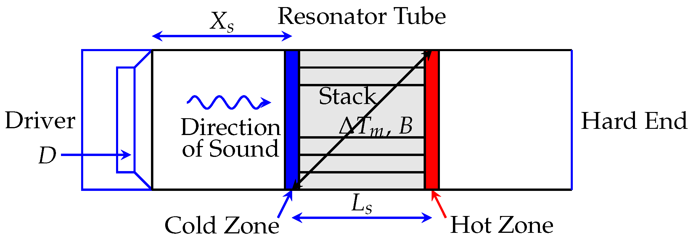
Figure 2.
DOE geometric representation. In each case, high levels are highlighted in blue, low levels in red.
Figure 2.
DOE geometric representation. In each case, high levels are highlighted in blue, low levels in red.
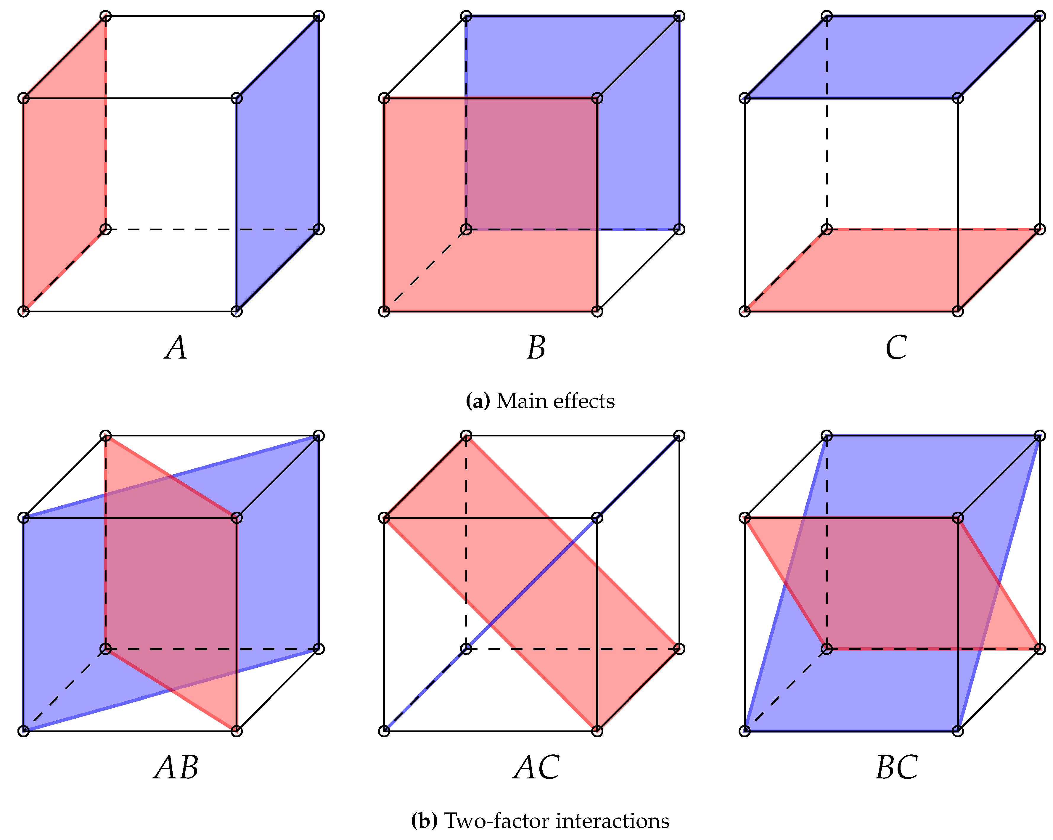
Figure 3.
Representative ’s response as a function of its dimensionless position and length .
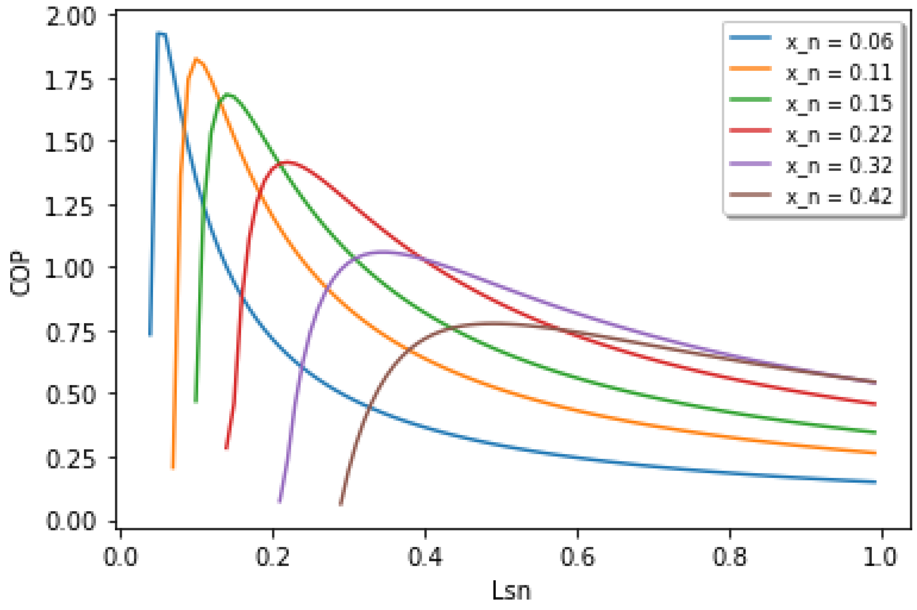
Figure 4.
Main factors for
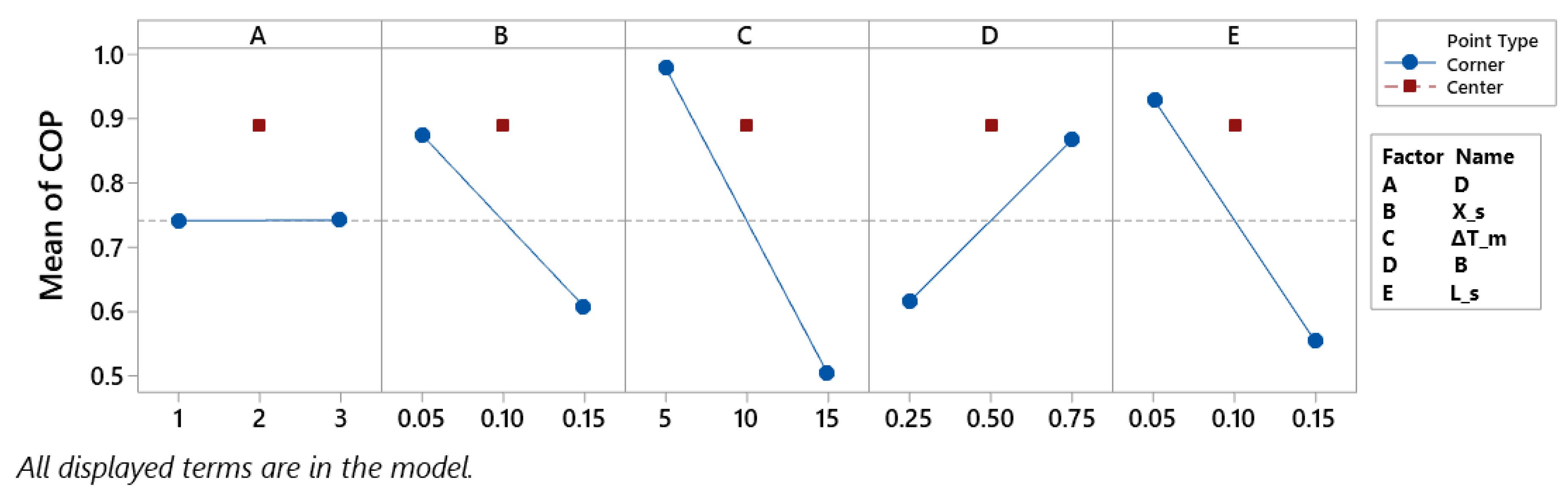
Figure 5.
Interaction factors
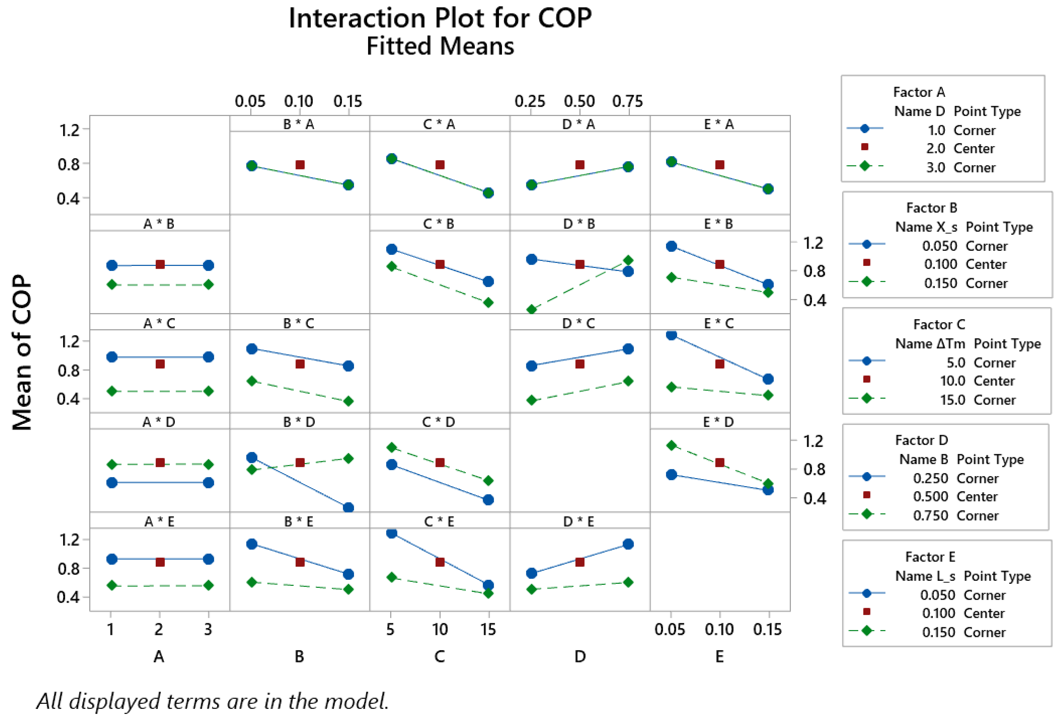
Figure 6.
COP’s Pareto Plot
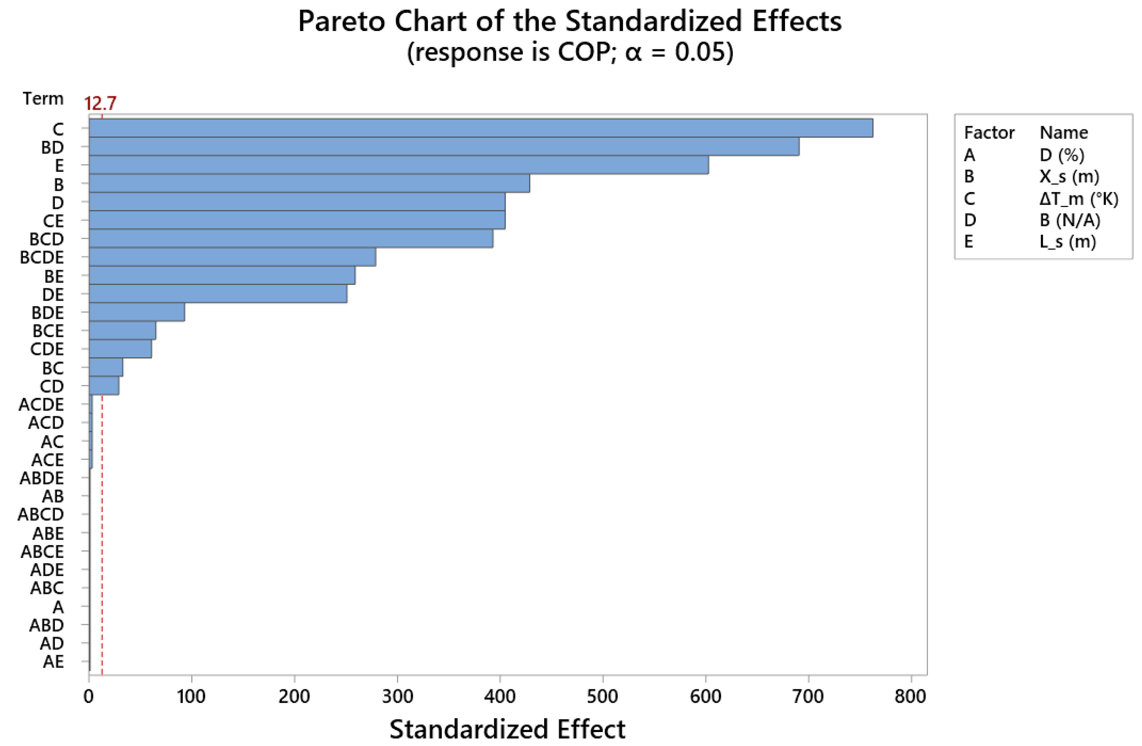
Figure 7.
COP’s Cube Plot

Figure 8.
COP’s Contours Plot Center Point Hold values
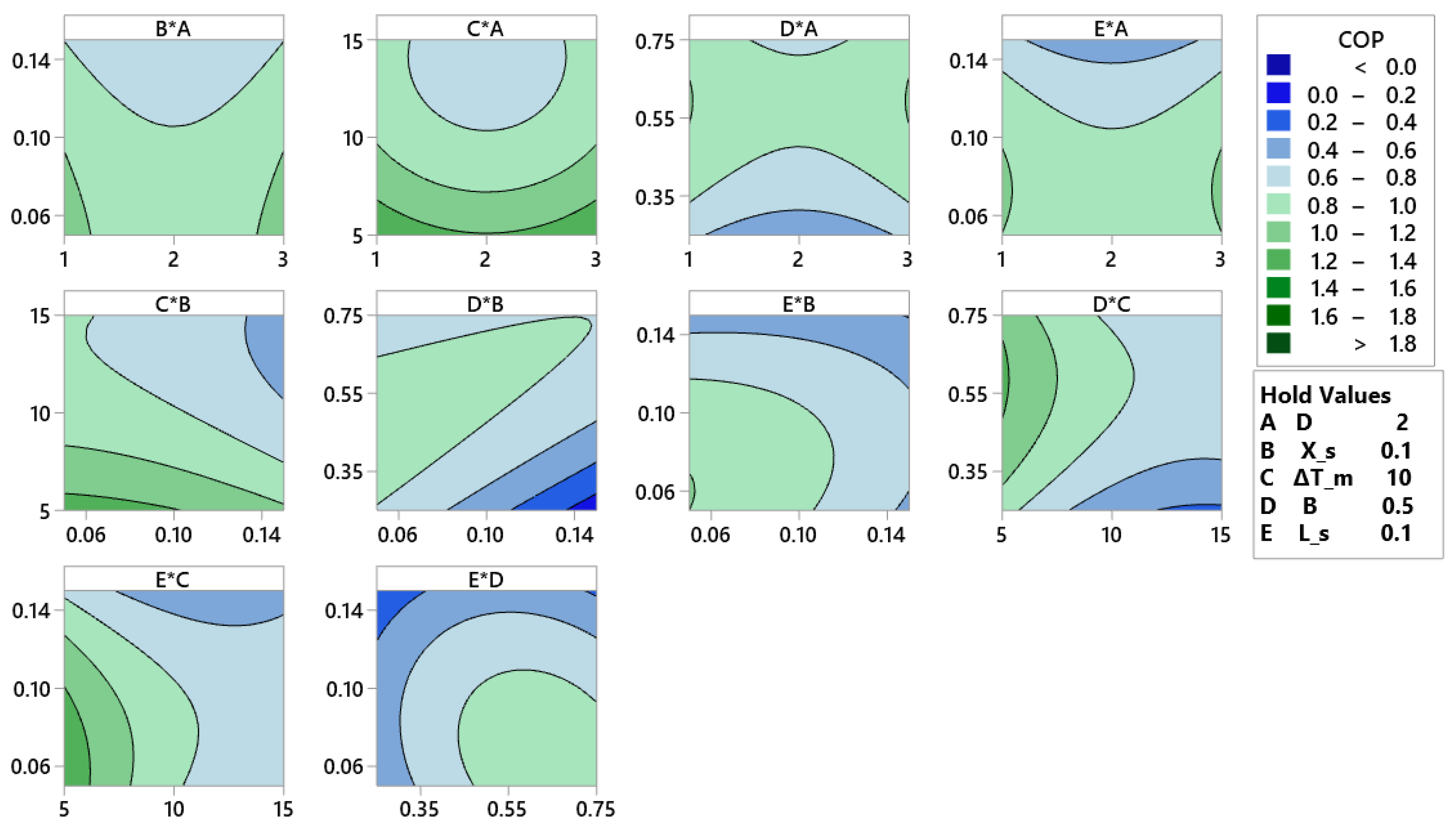
Figure 9.
COP’s Contours Plot Lower limits Hold values
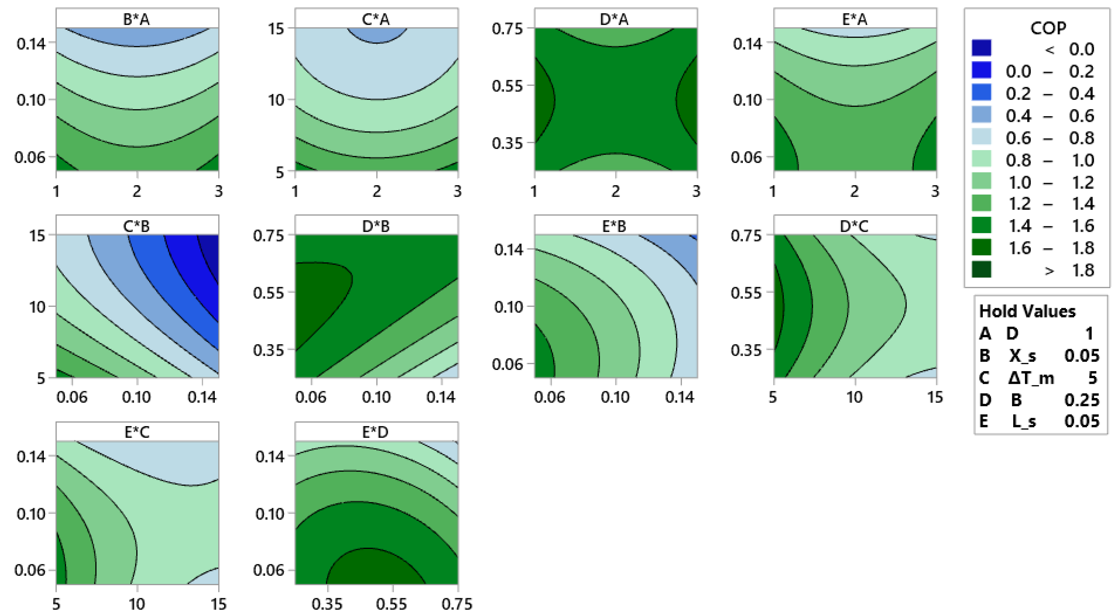
Figure 10.
COP’s Surface Plot Center Point Hold values

Figure 11.
COP’s Surface Plot Lower limits Hold values
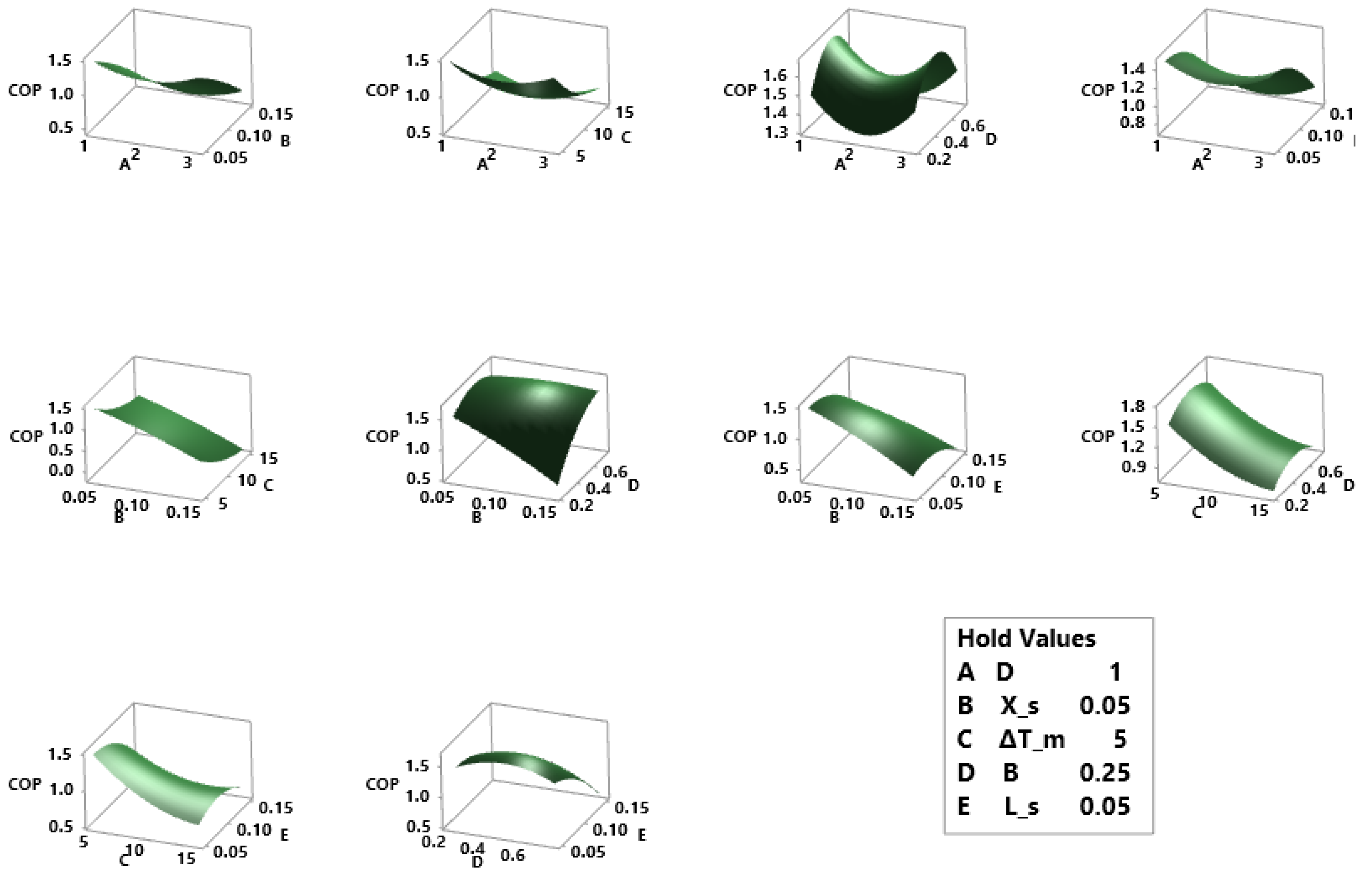
Figure 12.
’s result in Excel with the Transfer Function Obtained in MINITAB
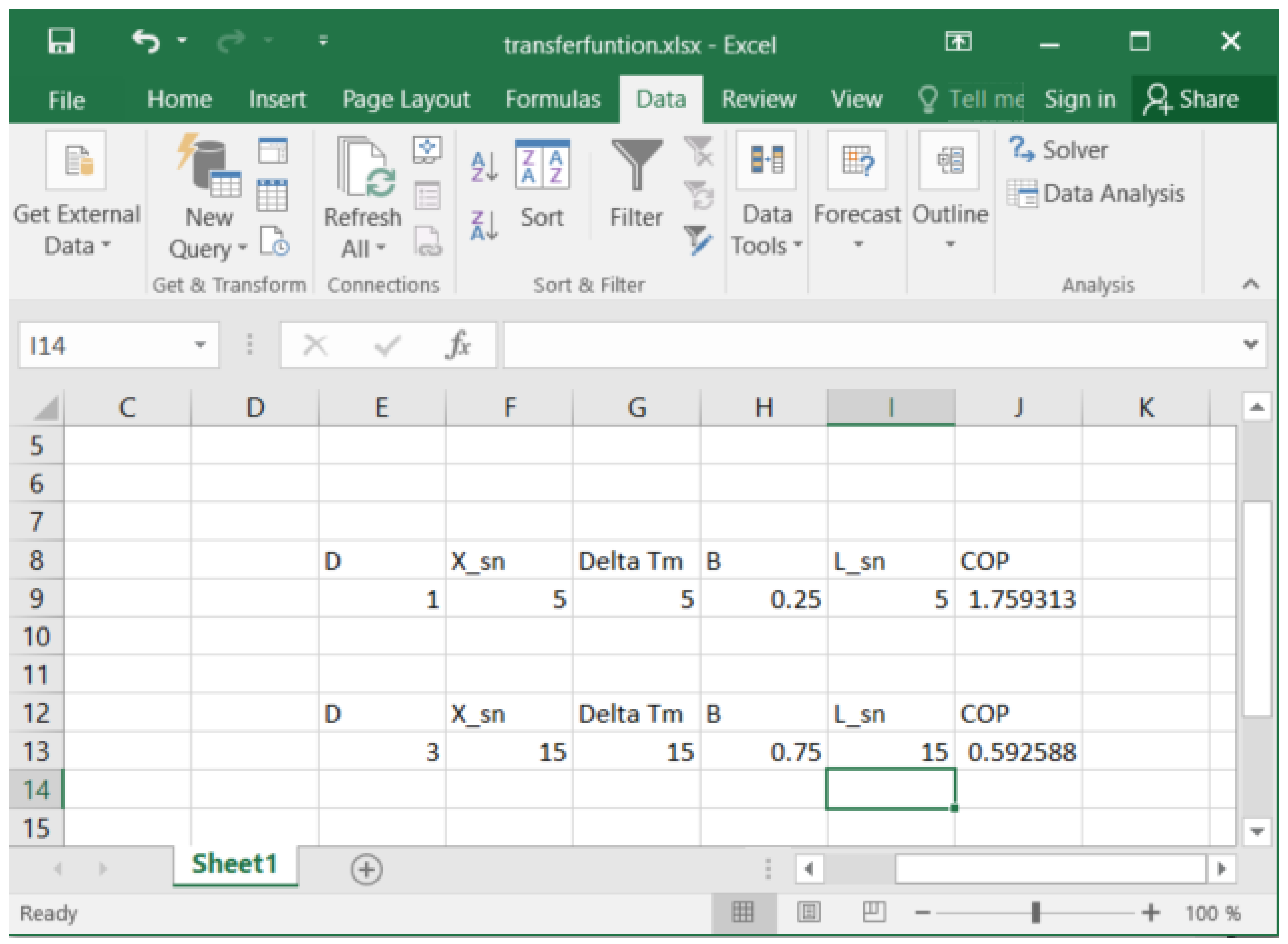
Table 1.
Parameters for optimizing thermoacoustic refrigerator [10].
Table 1.
Parameters for optimizing thermoacoustic refrigerator [10].
| Parameters | Definitions |
|---|---|
| Operational | Drive ratio D= |
| parameters | Dimensionless cooling power |
| Dimensionless acoustic power | |
| Dimensionless temperature difference | |
| Gas | Prandtl number =( |
| parameters | Dimensionless thermal penetration depth |
| Dimensionless viscous penetration depth | |
| Ratio of isobaric to isochoric specific heats | |
| Geometrical | Dimensionless stack length |
| parameters | Dimensionless stack position |
| Blockage Ratio |
Table 2.
Levels and intervals by factor used in the DOE.
| Factor | Name | Level | Units |
| Low - High | |||
| A | Drive Ratio (D) | - + | N/A |
| B | Dimensionless Stack Position () | - + | N/A |
| C | Dimensionless Temperature () | - + | N/A |
| D | Blocking Ratio (B) | - + | N/A |
| E | Dimensionless regenerator length () | - + | N/A |
Table 3.
Design of Experiments Orthogonal Array.
| Factors | |||||||||
| A | B | C | D | E | AB | AC | BC | ABC | |
| Run | |||||||||
| 1 | - | - | - | - | - | + | + | + | - |
| 2 | + | - | - | - | - | - | - | + | + |
| 3 | - | + | - | - | - | - | + | - | + |
| 4 | + | + | - | - | - | + | - | - | - |
| 5 | - | - | + | - | - | + | - | - | + |
| 6 | + | - | + | - | - | - | + | - | - |
| 7 | - | + | + | - | - | - | - | + | - |
| 8 | + | + | + | - | - | + | + | + | + |
| 9 | - | - | - | + | - | + | + | + | - |
| 10 | + | - | - | + | - | - | - | + | + |
| 11 | - | + | - | + | - | - | + | - | + |
| 12 | + | + | - | + | - | + | - | - | - |
| 13 | + | - | + | + | - | + | - | - | + |
| 14 | - | - | + | + | - | - | + | - | - |
| 15 | + | + | + | + | - | - | - | + | - |
| 16 | - | + | + | + | - | + | + | + | + |
| 17 | - | - | - | - | + | + | + | + | - |
| 18 | + | - | - | - | + | - | - | + | + |
| 19 | - | + | - | - | + | - | + | - | + |
| 20 | + | + | - | - | + | + | - | - | - |
| 21 | - | - | + | - | + | + | - | - | + |
| 22 | + | - | + | - | + | - | + | - | - |
| 23 | - | + | + | - | + | - | - | + | - |
| 24 | + | + | + | - | + | + | + | + | + |
| 25 | - | - | - | + | + | + | + | + | - |
| 26 | + | - | - | + | + | - | - | + | + |
| 27 | - | + | - | + | + | - | + | - | + |
| 28 | + | + | - | + | + | + | - | - | - |
| 29 | + | - | + | + | + | + | - | - | + |
| 30 | - | - | + | + | + | - | + | - | - |
| 31 | + | + | + | + | + | - | - | + | - |
| 32 | - | + | + | + | + | + | + | + | + |
Table 4.
Levels and intervals by factor used in the DOE.
| Factor | Name | Level | Units |
| Low - High | |||
| A | Drive Ratio (D) | 1 3 | % |
| B | Stack Position () | 0.05 0.15 | m |
| C | Temperature () | 5 15 | °K |
| D | Blocking Ratio (B) | 0.25 0.75 | N/A |
| E | Regenerator length () | 0.05 0.15 | m |
Table 5.
Design of Experiments Orthogonal Array with dimensional parameters
| Factors | A | B | C | D | E | |
| Name | D | B | ||||
| Units | % | m | °K | N/A | m | |
| Run | ||||||
| 15 | 1 | 0.15 | 15 | 0.75 | 0.05 | 0.59 |
| 30 | 3 | 0.05 | 15 | 0.75 | 0.15 | 0.45 |
| 25 | 1 | 0.05 | 5 | 0.75 | 0.15 | 0.48 |
| 10 | 3 | 0.05 | 5 | 0.75 | 0.05 | 1.28 |
| 16 | 3 | 0.15 | 15 | 0.75 | 0.05 | 0.59 |
| 27 | 1 | 0.15 | 5 | 0.75 | 0.15 | 0.88 |
| 3 | 1 | 0.15 | 5 | 0.25 | 0.05 | 0.40 |
| 21 | 1 | 0.05 | 15 | 0.25 | 0.15 | 0.60 |
| 19 | 1 | 0.15 | 5 | 0.25 | 0.15 | 0.40 |
| 1 | 1 | 0.05 | 5 | 0.25 | 0.05 | 1.76 |
| 11 | 1 | 0.15 | 5 | 0.75 | 0.05 | 1.74 |
| 8 | 3 | 0.15 | 15 | 0.25 | 0.05 | 0.13 |
| 26 | 3 | 0.05 | 5 | 0.75 | 0.15 | 0.49 |
| 12 | 3 | 0.15 | 5 | 0.75 | 0.05 | 1.74 |
| 13 | 1 | 0.05 | 15 | 0.75 | 0.05 | 0.93 |
| 23 | 1 | 0.15 | 15 | 0.25 | 0.15 | 0.13 |
| 29 | 1 | 0.05 | 15 | 0.75 | 0.15 | 0.45 |
| 22 | 3 | 0.05 | 15 | 0.25 | 0.15 | 0.60 |
| 28 | 3 | 0.15 | 5 | 0.75 | 0.15 | 0.89 |
| 17 | 1 | 0.05 | 5 | 0.25 | 0.15 | 0.89 |
| 4 | 3 | 0.15 | 5 | 0.25 | 0.05 | 0.40 |
| 18 | 3 | 0.05 | 5 | 0.25 | 0.15 | 0.89 |
| 14 | 3 | 0.05 | 15 | 0.75 | 0.05 | 0.93 |
| 2 | 3 | 0.05 | 5 | 0.25 | 0.05 | 1.76 |
| 6 | 3 | 0.05 | 15 | 0.25 | 0.05 | 0.61 |
| 5 | 1 | 0.05 | 15 | 0.25 | 0.05 | 0.61 |
| 32 | 3 | 0.15 | 15 | 0.75 | 0.15 | 0.58 |
| 7 | 1 | 0.15 | 15 | 0.25 | 0.05 | 0.13 |
| 33 | 2 | 0.10 | 10 | 0.50 | 0.10 | 0.89 |
| 9 | 1 | 0.05 | 5 | 0.75 | 0.05 | 1.28 |
| 20 | 3 | 0.15 | 5 | 0.25 | 0.15 | 0.40 |
| 31 | 1 | 0.15 | 15 | 0.75 | 0.15 | 0.59 |
| 24 | 3 | 0.15 | 15 | 0.25 | 0.15 | 0.13 |
Table 6.
Analysis of Variance.
| Source | DF | Seq SS | Contribution | Adj SS | Adj MS | F-Value | P-Value | Coeff. |
| Model | 31 | 7.25978 | 100.00% | 7.25978 | 0.23419 | 74939.71 | 0.003 | 5.5922 |
| Linear | 5 | 4.04327 | 55.69% | 4.04327 | 0.80865 | 258769.00 | 0.001 | |
| D | 1 | 0.00000 | 0.00% | 0.00000 | 0.00000 | 1.00 | 0.500 | 0.00656 |
| 1 | 0.57513 | 7.92% | 0.57513 | 0.57513 | 184041.00 | 0.001 | 0.41781 | |
| 1 | 1.81928 | 25.06% | 1.81928 | 1.81928 | 582169.00 | 0.001 | 0.33544 | |
| B | 1 | 0.51258 | 7.06% | 0.51258 | 0.51258 | 164025.00 | 0.002 | 5.5487 |
| 1 | 1.13628 | 15.65% | 1.13628 | 1.13628 | 363609.00 | 0.001 | 0.25144 | |
| 2-Way Interactions | 10 | 2.41728 | 33.30% | 2.41728 | 0.24173 | 77353.00 | 0.003 | |
| D* | 1 | 0.00000 | 0.00% | 0.00000 | 0.00000 | 1.00 | 0.500 | 0.000438 |
| D* | 1 | 0.00003 | 0.00% | 0.00003 | 0.00003 | 9.00 | 0.205 | 0.000563 |
| 1 | 0.00000 | 0.00% | 0.00000 | 0.00000 | 1.00 | 0.500 | 0.01625 | |
| 1 | 0.00000 | 0.00% | 0.00000 | 0.00000 | 1.00 | 0.500 | 0.000813 | |
| * | 1 | 0.00340 | 0.05% | 0.00340 | 0.00340 | 1089.00 | 0.019 | 0.024912 |
| *B | 1 | 1.49213 | 20.55% | 1.49213 | 1.49213 | 477481.00 | 0.001 | 0.69325 |
| * | 1 | 0.20963 | 2.89% | 0.20963 | 0.20963 | 67081.00 | 0.002 | 0.021062 |
| *B | 1 | 0.00263 | 0.04% | 0.00263 | 0.00263 | 841.00 | 0.022 | 0.44975 |
| * | 1 | 0.51258 | 7.06% | 0.51258 | 0.51258 | 164025.00 | 0.002 | 0.018988 |
| 1 | 0.19688 | 2.71% | 0.19688 | 0.19688 | 63001.00 | 0.003 | 0.22775 | |
| 3-Way Interactions | 10 | 0.53458 | 7.36% | 0.53458 | 0.05346 | 17106.60 | 0.006 | |
| D** | 1 | 0.00000 | 0.00% | 0.00000 | 0.00000 | 1.00 | 0.500 | 0.000038 |
| D**B | 1 | 0.00000 | 0.00% | 0.00000 | 0.00000 | 1.00 | 0.500 | 0.000750 |
| D** | 1 | 0.00000 | 0.00% | 0.00000 | 0.00000 | 1.00 | 0.500 | 0.000038 |
| D**B | 1 | 0.00003 | 0.00% | 0.00003 | 0.00003 | 9.00 | 0.205 | 0.001250 |
| D** | 1 | 0.00003 | 0.00% | 0.00003 | 0.00003 | 9.00 | 0.205 | 0.000062 |
| D*B* | 1 | 0.00000 | 0.00% | 0.00000 | 0.00000 | 1.00 | 0.500 | 0.002250 |
| **B | 1 | 0.48265 | 6.65% | 0.48265 | 0.48265 | 154449.00 | 0.002 | 0.047450 |
| **Ls | 1 | 0.01320 | 0.18% | 0.01320 | 0.01320 | 4225.00 | 0.010 | 0.001553 |
| *B* | 1 | 0.02703 | 0.37% | 0.02703 | 0.02703 | 8649.00 | 0.007 | 0.032450 |
| *B* | 1 | 0.01163 | 0.16% | 0.01163 | 0.01163 | 3721.00 | 0.010 | 0.024550 |
| 4-Way Interactions | 5 | 0.24329 | 3.35% | 0.24329 | 0.04866 | 15570.60 | 0.006 | |
| D***B | 1 | 0.00000 | 0.00% | 0.00000 | 0.00000 | 1.00 | 0.500 | 0.00005 |
| D*** | 1 | 0.00000 | 0.00% | 0.00000 | 0.00000 | 1.00 | 0.500 | 0.000002 |
| D**B* | 1 | 0.00000 | 0.00% | 0.00000 | 0.00000 | 1.00 | 0.500 | 0.000050 |
| D**B* | 1 | 0.00003 | 0.00% | 0.00003 | 0.00003 | 9.00 | 0.205 | 0.000150 |
| X**B* | 1 | 0.24325 | 3.35% | 0.24325 | 0.24325 | 77841.00 | 0.002 | 0.002790 |
| Curvature | 1 | 0.02137 | 0.29% | 0.02137 | 0.02137 | 6837.12 | 0.008 | 0.14844 |
| Error | 1 | 0.00000 | 0.00% | 0.00000 | 0.00000 | |||
| Total | 32 | 7.25979 | 100.00% |
- Note: DF, degree of freedom, Seq SS, Sequential SUM of squares,
- Adj SS, Adjust sum of squares, Adj MS, Adjust mean of squares,
- F=F-value, P=P-value, Coeff= Uncoded Coefficients
- S=0.0017678, R-Sq= 100.00 %, R-Sq(Adj) = 100.00%
Disclaimer/Publisher’s Note: The statements, opinions and data contained in all publications are solely those of the individual author(s) and contributor(s) and not of MDPI and/or the editor(s). MDPI and/or the editor(s) disclaim responsibility for any injury to people or property resulting from any ideas, methods, instructions or products referred to in the content. |
© 2024 by the authors. Licensee MDPI, Basel, Switzerland. This article is an open access article distributed under the terms and conditions of the Creative Commons Attribution (CC BY) license (http://creativecommons.org/licenses/by/4.0/).
Copyright: This open access article is published under a Creative Commons CC BY 4.0 license, which permit the free download, distribution, and reuse, provided that the author and preprint are cited in any reuse.


