1. Introduction
Throughout the history of mathematical modeling, traditional calculus has been the primary tool for explaining the behavior of various phenomena, ranging from the physics of kinetics and electromagnetism to the spread of diseases in biology and numerous other systems in between. For a significant period, it was widely accepted that classical calculus sufficed to model these systems comprehensively. However, contemporary research suggests that a more generalized form of calculus, known as fractional calculus, offers superior modeling capabilities for these phenomena [
1,
2,
3,
4,
5]. The concept that fractional calculus might provide more accurate models than traditional calculus is still under investigation. The immediate implications of these enhanced models include a more detailed understanding of the specifics behind systematic evolutions and anomalous behaviors in many physical problems. Often, such nuances are overlooked when using traditional calculus models. By comprehending fractional calculus, we can elucidate patterns in physical phenomena that traditional methods have not yet captured. This deeper insight enhances our understanding of these problems and may drive innovative advancements in their modeling techniques [
6,
7].
A reaction-diffusion model is a mathematical framework used to describe the behavior of chemical or biological systems in which substances interact (reaction) and spread out in space (diffusion). This type of model is instrumental in understanding a wide range of phenomena, from chemical reactions and biological pattern formation to ecological dynamics and neural activity. A typical reaction-diffusion system is governed by a set of partial differential equations (PDEs) of the form
where
represents the concentration of the
th substance at position
and time
,
is the diffusion coefficient of the
th substance, indicating how it spreads through space.
denotes the Laplacian operator, representing spatial diffusion and
is the reaction term, describing the interactions between the substances, often involving nonlinear functions of the concentrations.
Equation of the form (1) has been applied to model many physical phenomena. For example, in chemistry, reaction-diffusion models describe how chemical species react and diffuse in a medium. Classic examples include the Belousov-Zhabotinsky reaction, which exhibits oscillatory behavior, and the formation of patterns in chemical gardens [
8]. Reaction-diffusion models are fundamental in developmental biology, explaining how patterns such as animal coat markings, spatial organization of cells, and morphogenesis (the development of the structure of an organism) arise [
8,
9]. Alan Turing’s seminal work introduced the concept that reaction-diffusion systems can generate stable patterns, known as Turing patterns [
10]. In ecology, these models describe the spread of species, the interaction between predator and prey populations, and the dynamics of ecosystems [
11,
12,
13,
14,
15,
16]. They help understand phenomena like population waves, species invasion, and spatial distribution of organisms [
17,
18]. In neuroscience, reaction-diffusion models are used to simulate the propagation of electrical signals in neurons and the dynamics of neurotransmitter diffusion in the brain. They also model the activity patterns in neural networks, explaining wave-like behaviors and pattern formation in brain activity.
A fractional reaction-diffusion equation is an extension of the classical reaction-diffusion equation, incorporating the concept of fractional calculus. This approach allows for more accurate modeling of anomalous diffusion and non-local interactions, which are observed in many complex systems where the assumptions of standard diffusion are not valid. The benefits of fractional differential equations are particularly evident in modeling the mechanical and electrical characteristics of real materials, as well as in describing the rheological properties of rocks. Additionally, they are extensively used in various scientific and engineering disciplines, including fluid dynamics, practical applications, diffusive transport analogous to diffusion, electrical circuits, electromagnetic theory, and probability [
1,
2,
5,
19,
20].
The fractional reaction-diffusion equation can be written as
with conditions
where
is the fractional derivative of order
, defined by the Caputo operator as
Clearly, the Caputo derivative
is made up of derivatives
and
, that is,
Given this make-up, it follows that
Theorem 1.1 The Caputo reaction-diffusion equation (2) is equivalent to integro- differential equation
where
and
denotes the Riemann-Liouville fractional integral derivative of order
formulated as
Readers are referred to [
21] and (4), for details of the proof.
Numerical methods play a crucial role in approximating solutions for time-fractional reaction-diffusion equations, which model processes exhibiting anomalous diffusion and memory effects. Among the popular techniques, finite difference methods (FDM) are widely utilized due to their simplicity and straightforward implementation [
22,
23]. These methods discretize the time-fractional derivatives using schemes like the Grunwald-Letnikov or L1 approximation, enabling the transformation of the continuous problem into a system of algebraic equations. The stability and convergence of these methods are often analyzed to ensure accurate solutions, with recent studies focusing on improving their efficiency and accuracy for complex problems. In contrast, finite volume methods (FVM) and spectral methods offer alternative approaches that can provide higher accuracy, especially for problems with complex geometries or requiring high-resolution solutions [
23,
24]. Finite volume methods, which conserve fluxes across control volumes, are particularly effective for handling heterogeneous media and ensuring conservation laws. Spectral methods, leveraging orthogonal polynomials or Fourier series, provide exponential convergence for smooth problems and have been adapted for fractional derivatives using fractional calculus [
25,
26]. Recent advancements include hybrid methods that combine FDM, FVM, implicit-explicit (IMEX), spectral methods and a family of Adams-Bashforth methods [
27,
28], to leverage their respective strengths, offering enhanced stability and accuracy for simulating time-fractional reaction-diffusion processes in various applications [
29,
30].
The rest of the paper is organized as follows. In
Section 2, we explore various numerical approximation methods and analyze their convergence properties.
Section 3 introduces three significant dynamic systems and discusses their applications in various fields.
Section 4 focuses on high-dimensional numerical experiments that examine pattern formation arising from these dynamic examples. Finally, the conclusion summarizes the findings and suggests future research directions.
2. Numerical Methods
Here, we provide details of numerical approximation of the Caputo reaction-diffusion equation. To discretize, we let
to be a equal mesh on integration interval
, where
with
. In the same manner, we let
be a uniform mesh of interval
, where
with
. Assume
and
are the grid functions on
We use a similar notation as suggested in [
31]:
It is not difficult to verify that
According to Lubich [
32], there exists a numerical method for approximating the Riemann-Liouville (RL) fractional integral.
Lemma 2.1
Suppose with and continuous, then
where
for
By applying the above lemma, one gets a finite difference method for the approximation of (5) as
where
stands for the numerical solution of
. The terms
and
are respectively substituted with the central difference scheme and classical backward Euler method.
Next, we rearrange the method above to get
where
We shall refer to this as first method. Likewise, using the Crank-Nicolson method to discretize (6) results in another scheme
It should be mentioned that either of the first (9) or (10) schemes forms a tridiagonal system of linear equations, which can be solved at each time step using the Thomas algorithm.
2.1. Convergence and Solvability Properties of the Difference Schemes
Hereafter, let denote a positive constant that does not depend on or , though its value may vary in different contexts. We begin by applying the Gershgorin circle theorem (GCT) to demonstrate the solvability of numerical formulae (9) and (10).
Theorem 2.1 The schemes (9) and (10) are uniquely-solvable.
Proof. Since the two methods are similar, we present the solvability of only scheme (9) here in what follows
Bear in mind that we adopt the homogeneous boundary conditions for our Caputo time-fractional reaction-diffusion problem (2), which allows equation (11) to take the matrix form
By the GCT, the matrice is invertible, which proves that scheme (9) is solvable.
The subsequent lemma, which addresses the nonnegative nature of specific real quadratic forms with a convolution structure, is attributed to [
31]. It is crucial here for the convergence analysis study.
Lemma 2.2
Suppose is monotonically decreasing function of positive real numbers with condition then for any integer and real vector satisfies that
Lemma 2.3 The sequence defined in (7) holds for
Since and then
The proof is completed.
2.2. Analysis of Convergence for Scheme (9)
Assume
then for (9), we obtain
Theorem 2.2 Suppose and are the numerical solutions to time-fractional reaction-diffusion problems (2) and (9) respectively, and that meets the smoothness criteria of (17). Then, for sufficiently small and ,
where
.
Proof. By taking (9) from (18), one gets the error equation
where
Next, we multiply on both sides of (20) by
and add up for
from 1 to
, to get
Applying the inequality
we have
By summing up the inequities above results to
where
and have applied the inequality
and Lemma 11 result. Thus the condition (19) holds.
Using a method analogous to that employed in the convergence proof, we can demonstrate the stability of the scheme (9), that is,
2.3. Analysis of Convergence for Scheme (10)
Assume and are continuous and differentiable on interval , with . This assumption is likely the minimal condition required for the existence of the Caputo-in-time derivative of order (for subdiffusion process) or (in the case of superdiffusion scenarios).
For any
satisfying
and
as
. We will approximate
numerically. We can generalize the result in [
33] to the formulas as follows
For any
that satisfies
and
as
, we approximate
numerically. The result from [
33] can be generalized to the following formulas.
and
Since
for
then results to
Furthermore, we can verify that
When equations (7), (26) and (27) are combined, we have
Next, we report the error estimate for the second scheme (10) as follows.
Theorem 2.3
Suppose that the solution to Caputo reaction-diffusion equation (2) meets the given smoothness requirements. Denote as the solution of (2) and be the solution of numerical scheme (10). Then, as and independently approach zero
Proof. Taking (7) from (28), we get
where
We multiply
on both sides of equation (30), and adding up in terms of
, to have
For superdiffusive process (
), the series
in (32) is convergent, which satisfies
In the same way, it can be verified that the numerical scheme (10) is stable and satisfies the inequality condition
Based on the error estimates (19) and (29), both schemes exhibit first-order accuracy in time and second-order accuracy in space. However, Scheme 2 has less stringent smoothness requirements compared to Scheme 1, allowing it to be applied across a wider range of scenarios.
In the works [
31,
33,
34], numerical discussions are presented for a partial integro-differential equation similar to (6) with a fractional order of
. Sanz-Serna introduces a temporal semi-discrete first-order algorithm. Lopez proposes a difference scheme based on the backward Euler method, with an error estimation of
. Tang employs the Crank-Nicolson method and the product trapezoidal method to develop a difference scheme with an accuracy of
. However, it remains uncertain whether this approach can be extended to any
.
3. Model Equations
In these sections, we present and briefly discuss some practical reaction-diffusion models that continue to be of significant interest due to their wide-ranging applications in various fields. These models are essential for understanding complex systems in both natural and engineered environments.
3.1. Allen-Cahn Equation
The Allen-Cahn equation, named after John W. Cahn and Sam Allen, is a pivotal reaction-diffusion equation in mathematical physics. This equation is crucial for modeling the process of phase separation in multi-component alloy systems, which includes phenomena such as order-disorder transitions. Phase separation is a fundamental process where a homogeneous mixture of components evolves into distinct regions or phases, each enriched in different components. This process is driven by the system’s tendency to minimize its free energy. The Allen-Cahn (AC) equation provides a mathematical framework to describe the temporal evolution of this separation, capturing the complex interplay between reaction kinetics and diffusion [
35].
Mathematically, the Allen-Cahn equation is typically written as:
Here, represents the order parameter, which indicates the local state of the system (e.g., the concentration of a particular component). The term represents the diffusion term, where is the Laplacian operator, reflecting how the order parameter spreads out over time. The function is a nonlinear term derived from the free energy of the system, often taking the form of the derivative of a double-well potential, such as .
In reaction-diffusion dynamics, the AC equation combines the effects of local reactions ()described by
and diffusion (described by
). This combination allows it to model the competition between different phases in a material. In multi-component alloy systems, the equation is particularly useful for studying order-disorder transitions. These transitions occur when a system changes from a disordered state, where components are randomly distributed, to an ordered state, where components are arranged in a regular pattern. The equation also describes the dynamics of interfaces between different phases. As time progresses, these interfaces move and evolve according to the balance between diffusive spreading and the local reaction kinetics [
36]. In materials science, the Allen-Cahn equation is widely used to simulate and understand the microstructural evolution of alloys. For instance, it can predict how different phases nucleate, grow, and coarsen over time, providing insights into the material’s properties.
The Allen-Cahn equation has been extensively studied both analytically and numerically. Analytical approaches often involve studying the stability and bifurcation of solutions, which provide insights into the conditions under which different phases form and evolve. Numerical simulations, on the other hand, allow for the detailed visualization of phase separation processes and the exploration of complex scenarios that are analytically intractable. The AC equation is closely related to the Cahn-Hilliard equation, which also describes phase separation but focuses on conserved quantities. While the Allen-Cahn equation models non-conserved order parameters (like the local state of order), the Cahn-Hilliard equation deals with conserved quantities (like concentration). Both equations are fundamental in the study of pattern formation and are used to describe different aspects of phase separation dynamics.
3.2. The KPP-Fisher Equation
In mathematical physics, the KPP-Fisher equation, named after Andrey Kolmogorov, Ivan Petrovsky, Nikolai Piskunov, and Ronald Fisher, is a prominent partial differential equation. It is also commonly referred to as the KPP equation, the Fisher equation [
37], or the Fisher-KPP equation [
38,
39]. This equation is significant in various fields, including population genetics, ecology, and the study of reaction-diffusion systems.
The general KPP-Fisher equation is typically expressed as:
Here, represents the density of the population or the concentration of a chemical substance at position and time . The term is the Laplacian operator that represents the diffusion component, where is the diffusion coefficient, indicating how the substance spreads out in space. The term is the reaction component, where is the growth rate of the population or reaction rate of the chemical substance. It should be noted that whenever and , we recover the Allen-Cahn equation (35). The KPP-Fisher equation is related to other reaction-diffusion equations like the Allen-Cahn equation and the Cahn-Hilliard equation. While the KPP-Fisher equation primarily focuses on traveling wave solutions and logistic growth, the Allen-Cahn equation models phase separation with non-conserved order parameters and the Cahn-Hilliard equation deals with conserved quantities in phase separation processes.
The Fisher equation was originally derived to describe the spread of an advantageous gene in a population. The term models logistic growth, where grows quickly when it is small, but slows down as it approaches the carrying capacity (normalized to 1). One of the notable features of the KPP-Fisher equation is its ability to describe traveling wave solutions. These are wave-like fronts that move with a constant speed, representing the spread of a gene, population, or chemical concentration through space over time. The minimum speed of these waves is given by . In an ecological context, the equation models the spread of a species through a habitat. It accounts for both the natural diffusion of the species and their growth and competition dynamics. Similarly in the context of chemical reactions, the equation describes the spread of reactants in a medium, combining the effects of chemical kinetics and molecular diffusion.
Analytically, the KPP-Fisher equation has been studied for its traveling wave solutions, stability of these waves, and the long-term behavior of solutions. Understanding the minimum wave speed and the conditions for wave formation are key analytical challenges. Numerical simulations are extensively used to explore the dynamics of the equation in more complex scenarios, such as heterogeneous environments or higher-dimensional spaces.
3.3. Ginzburg-Landau Equation
The Ginzburg-Landau equation, named after Vitaly Ginzburg and Lev Landau, is a fundamental equation in the field of nonlinear dynamics and pattern formation. It describes the evolution of small disturbances near a finite wavelength bifurcation, where a system transitions from a stable to an unstable state. This equation plays a critical role in understanding how complex patterns emerge in various physical, chemical, and biological systems.
The Ginzburg-Landau equation is typically given as [
40,
41]
where
is the complex amplitude of the disturbance,
is a small parameter representing the distance from the bifurcation point,
is a coefficient related to the spatial diffusion of the amplitude, and
is nonlinear coefficient. The real part of
is particularly important for describing the physical aspects of the system’s state.
At the onset of a finite wavelength bifurcation, the system becomes unstable for a critical wavenumber
which is non-zero. This instability leads to the growth of disturbances characterized by this wavenumber. Near the bifurcation, the disturbances evolve with a Fourier mode corresponding to
and a slowly varying amplitude
. The Ginzburg-Landau equation governs the dynamics of this amplitude
, capturing how the disturbances grow, saturate, and interact over time. It should be mentioned that for oscillatory behavior,
satisfies the novel complex Ginzburg-Landau equation [
42] The Ginzburg-Landau equation is typically given as
where
and
are treated as real constants. The solution of (38) often results to two important modes. The non-oscillatory modes which represent steady-state patterns that do not change in time once they have fully developed. The disturbances grow until they reach a stable amplitude and form stationary spatial structures, and the oscillatory modes which lead to time-dependent patterns that oscillate as they evolve. The amplitude
varies not only in space but also in time, leading to complex temporal behavior.
The Ginzburg-Landau equation is crucial in the study of pattern formation. It describes how simple initial disturbances can grow and form intricate spatial and temporal patterns [
43]. This is observed in a wide range of systems, from chemical reactions (like the Belousov-Zhabotinsky reaction) to fluid dynamics (such as Rayleigh-Benard convection). In the context of superconductivity, the equation helps describe the behavior of the order parameter near the critical temperature. It provides insights into the formation of vortices and other phenomena in superconducting materials. For nonlinear optics, the GL equation models the propagation of light in nonlinear media, explaining the formation of optical patterns and solitons in lasers and other optical systems, and in biology, it helps understand the development of patterns in animal skins, the dynamics of populations, and other phenomena where spatial and temporal variations are critical.
Analytically, the Ginzburg-Landau equation is studied to understand the stability and bifurcation behavior of solutions. Researchers investigate how solutions change as parameters like
and
vary, and how nonlinear interactions lead to saturation and pattern formation. Numerically, simulations of the Ginzburg-Landau equation reveal detailed behavior of the amplitude
over time and space [
44]. These simulations help visualize complex phenomena that are analytically intractable, providing deeper insights into the dynamics of the system.
4. Numerical Experiments and Results
In this section, we carry out some numerical experiment to investigate dynamic behavior of the Allen-cahn equation (35), KPP-Fisher equation (36) and the Ginzburg-Landau equation (38) in one, two and three dimensional spaces on Alienware computer using the Matlab R2021a software.
At first, one requires to justify the performance of schemes (9) and (10) before solving the main problems. To achieve this, we consider the Caputo time-fractional diffusion problem (2) as
With choice
we compute with exact solution
. The maximum error
is displayed in
Table 1 for different instances of
and fractional power
with both schemes.
For all the experiments, we utilize the homogeneous (zero-flux) boundary conditions and the following initial conditions
and
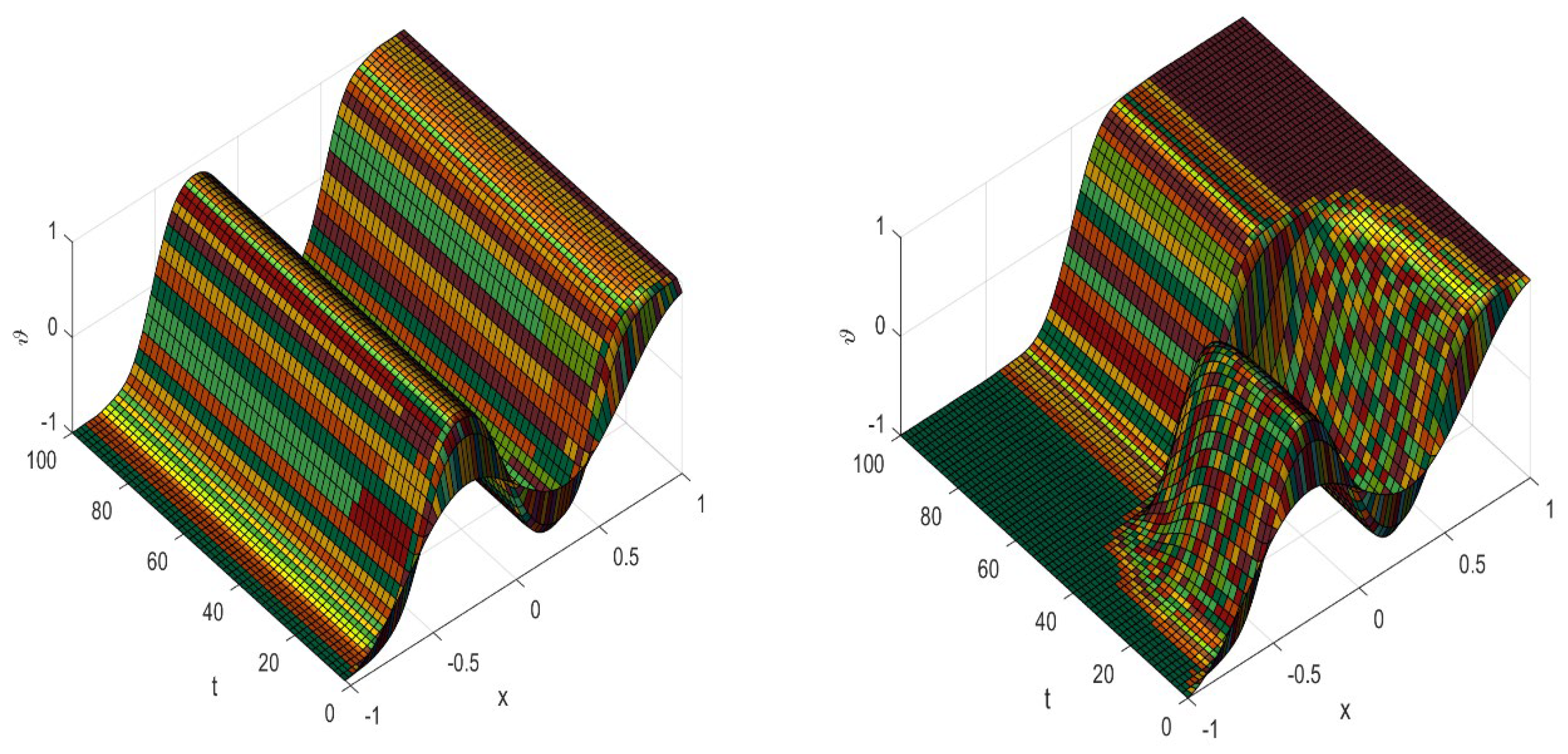
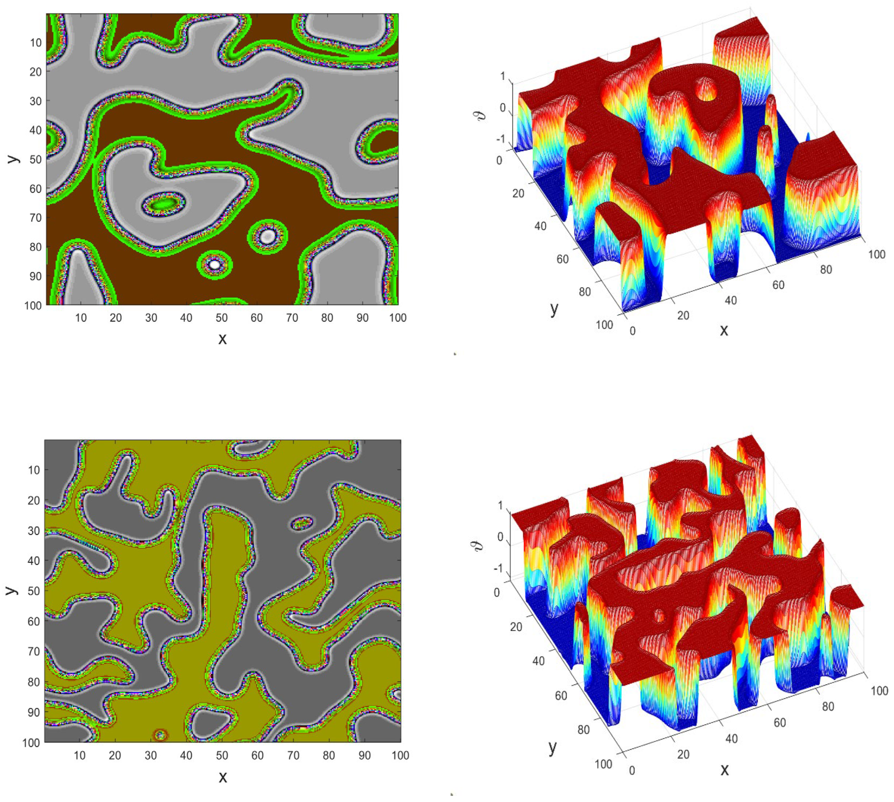
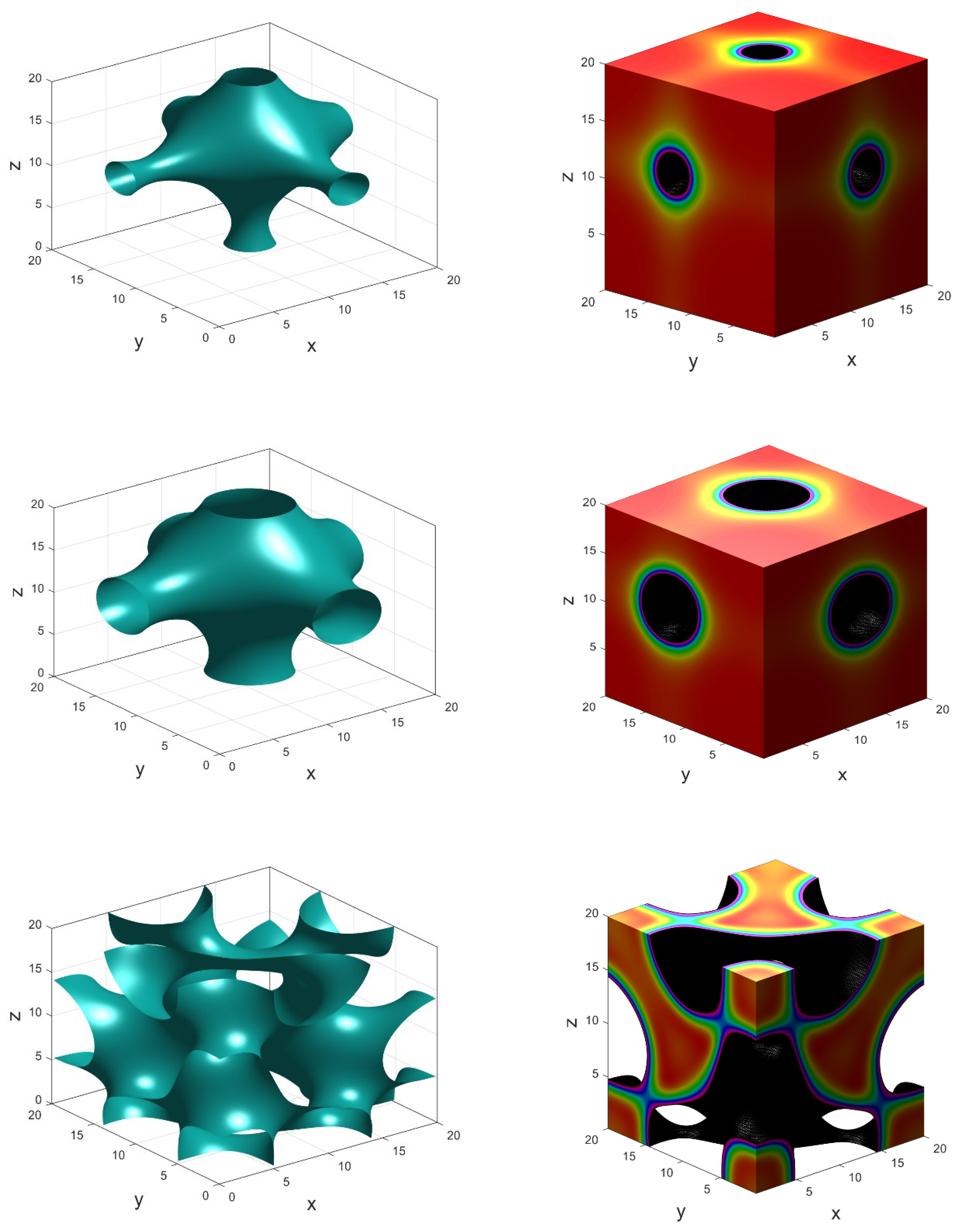
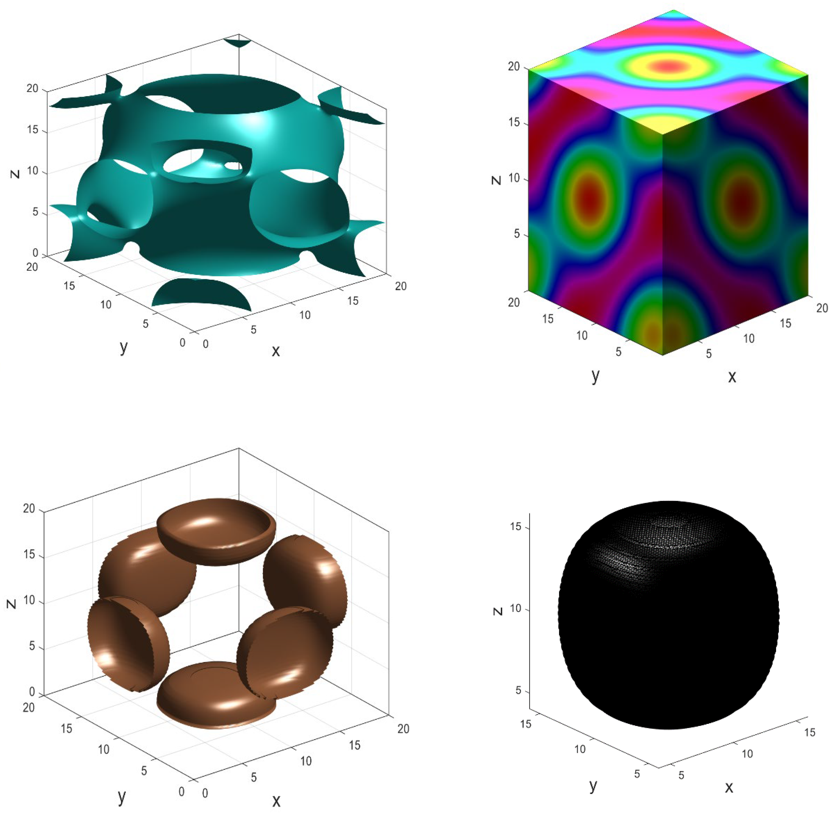
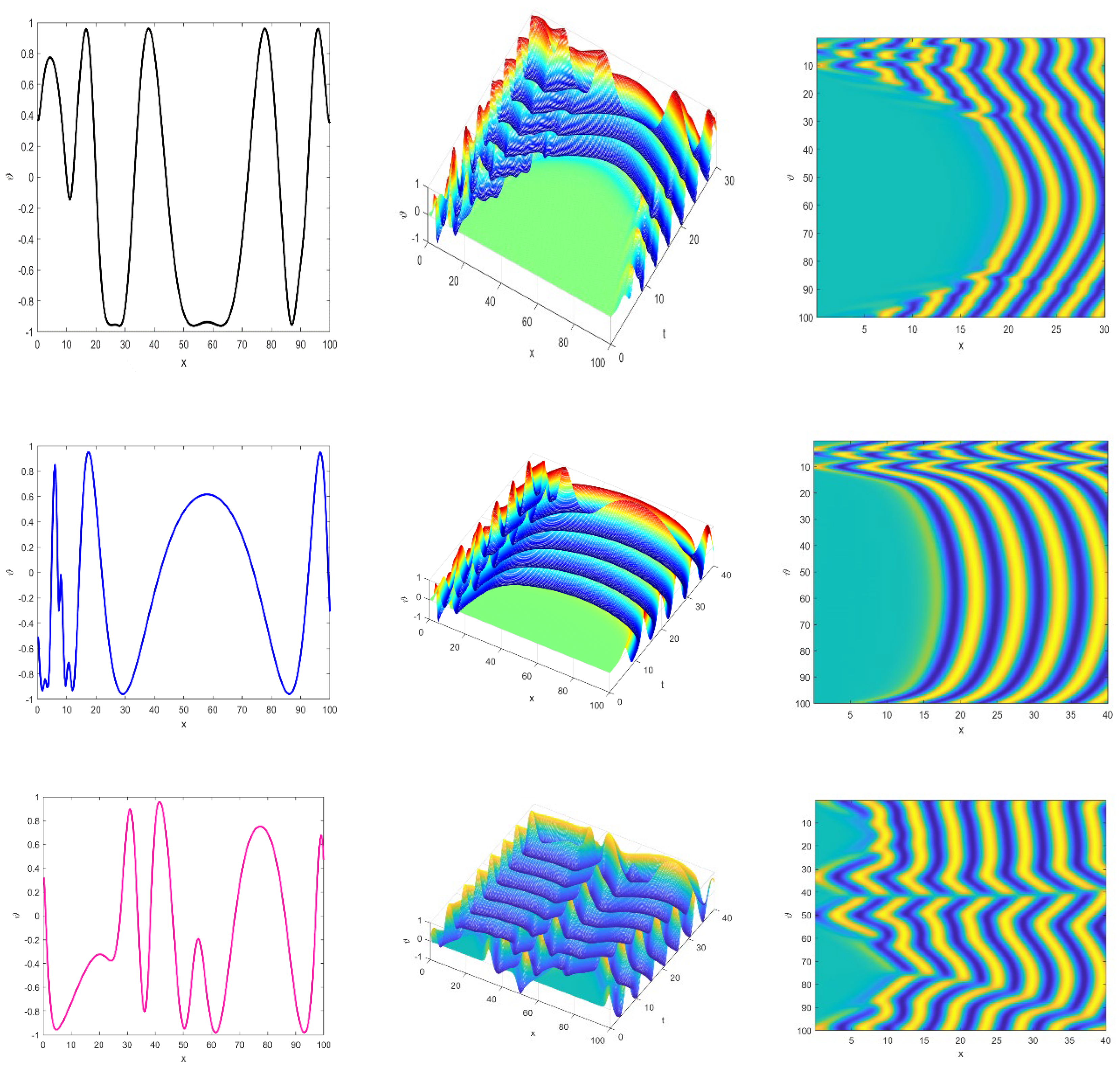
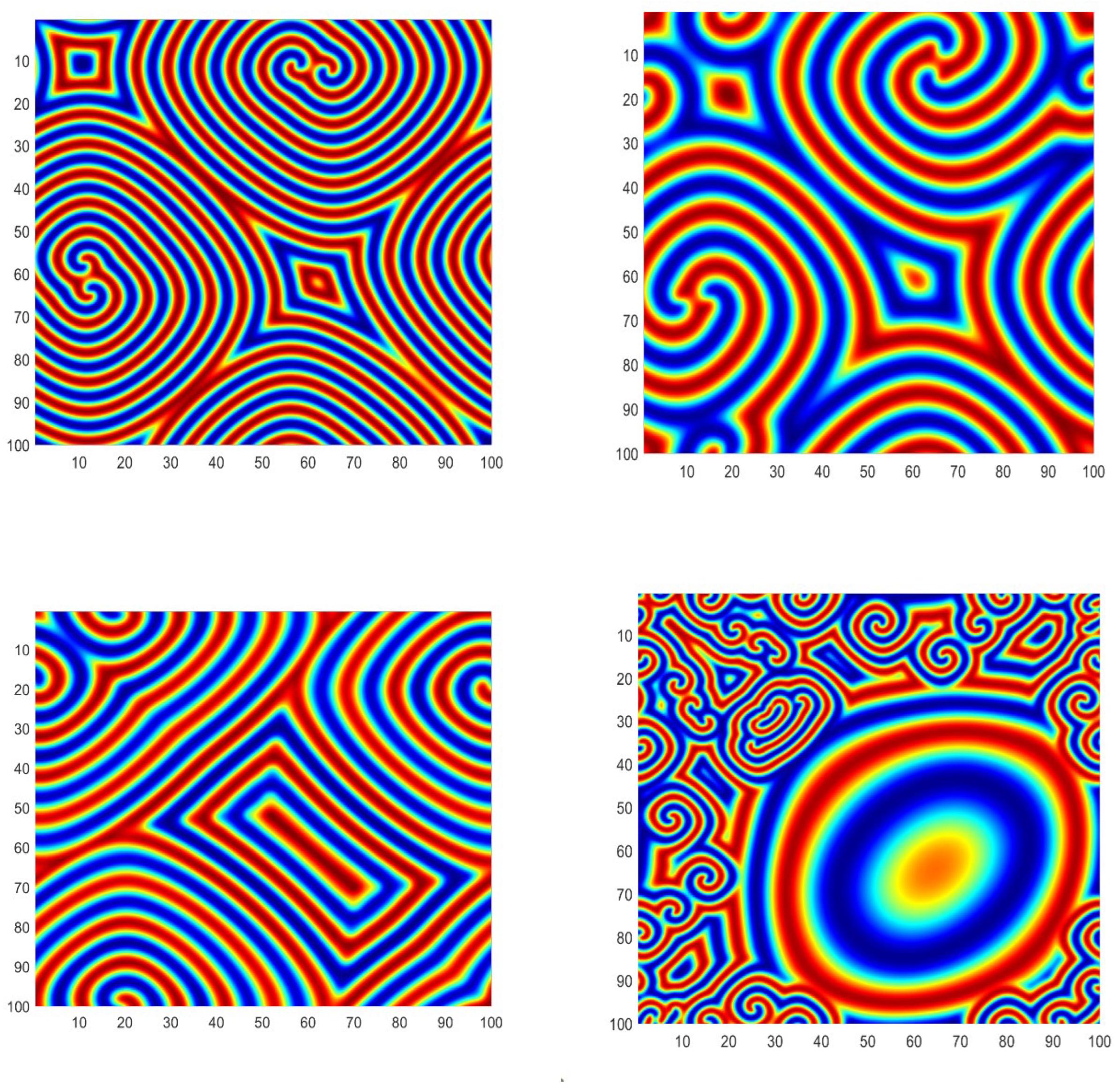
The dynamic behaviour of the fractional Allen-Cahn equation (35) in 1D, 2D and 3D are displayed in
Figure 1,
Figure 2 and
Figure 3, respectively, with
.
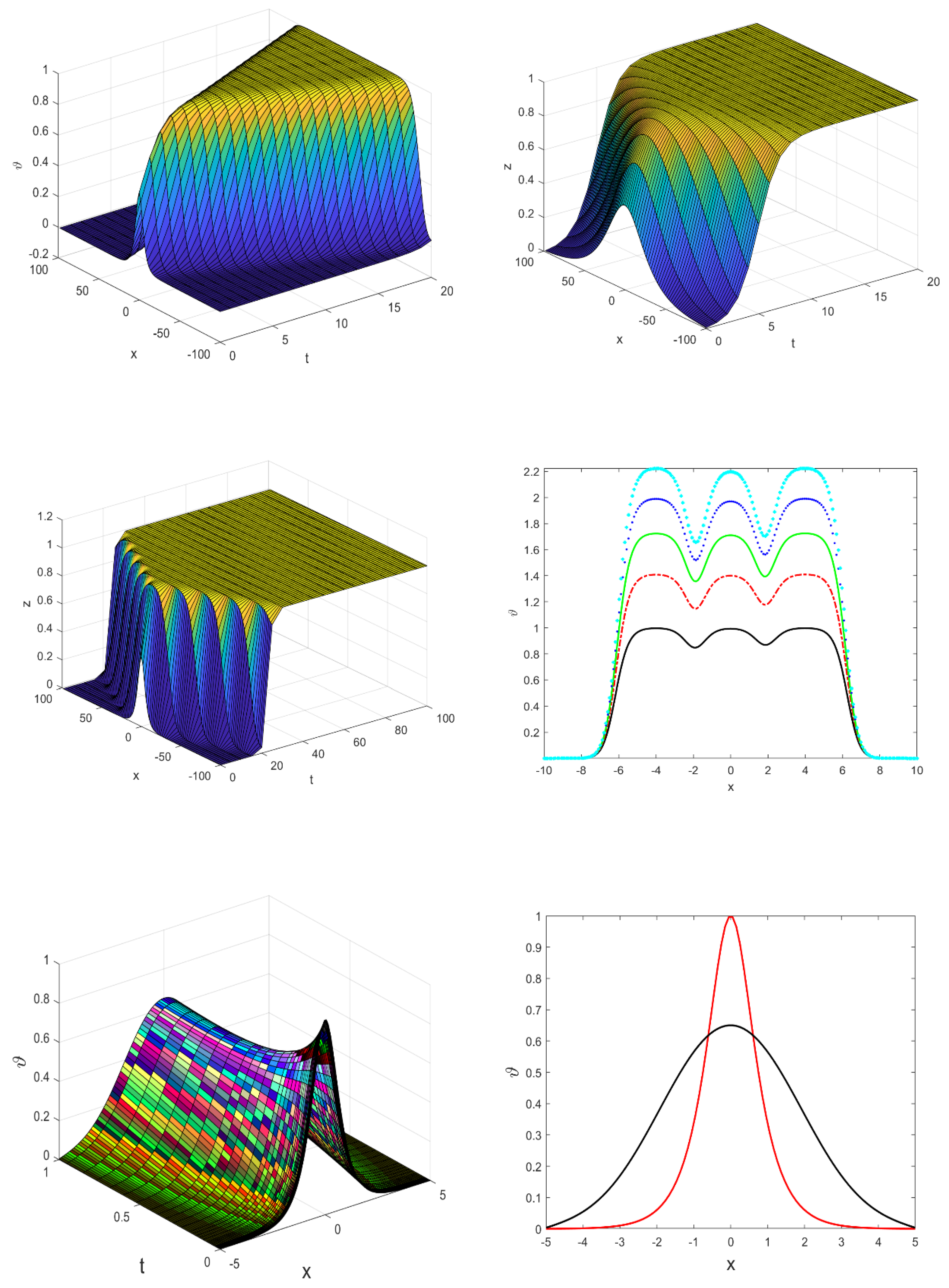
Figure 1 is obtained for varying
and
depicts the exact behavior of the standard Allen-Cahn equation in [
45]. In the experiments, the equation exhibits stable equilibria at
and an unstable equilibrium at
. A notable aspect of this equation is its metastability. Solutions close to
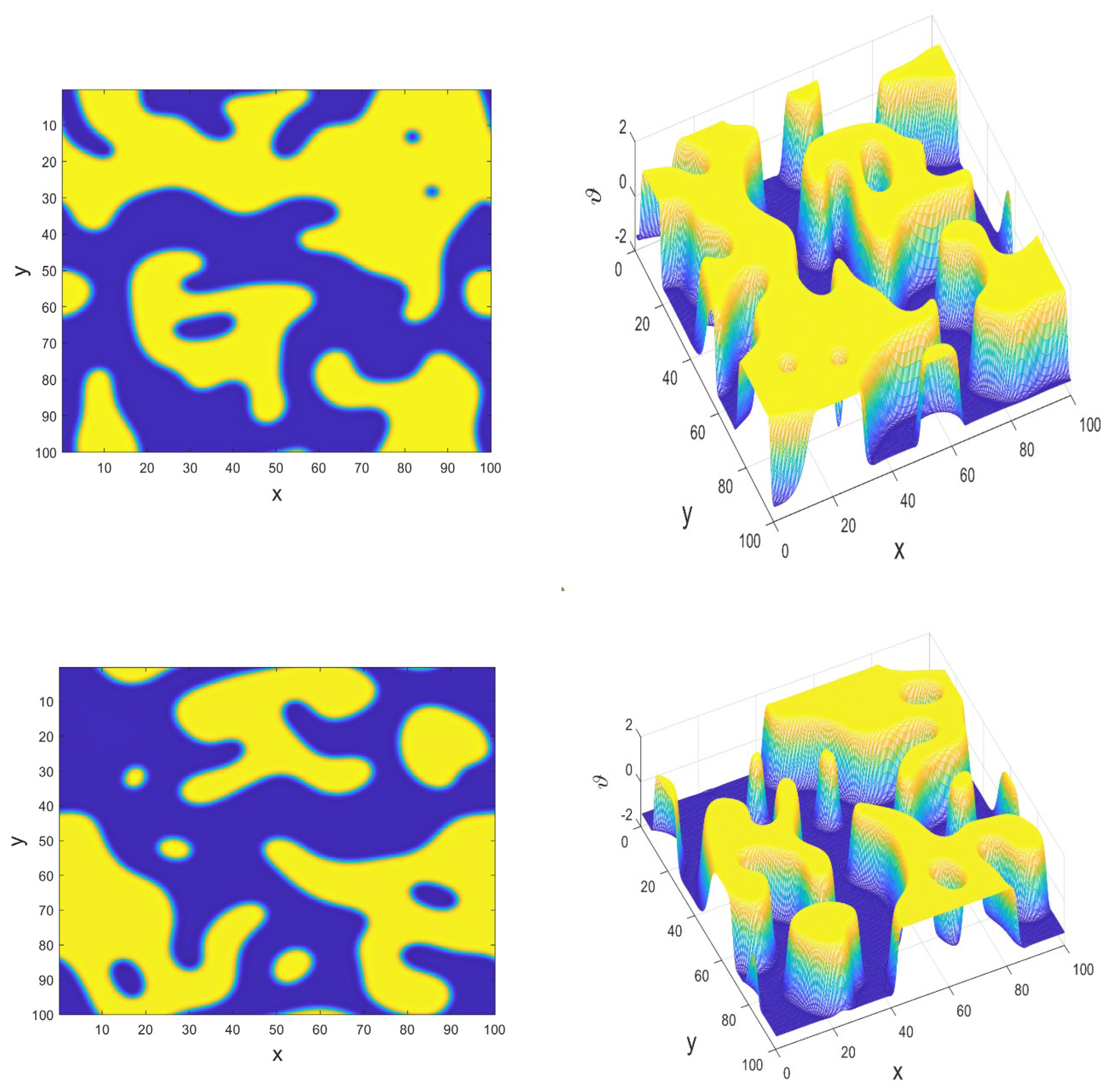
tend to have flat surface, with the interface between these regions remaining stable for extended periods before experiencing a sudden change. In 2D, we observed different spiral patterns as shown in
Figure 2. The 3D dynamics for subdiffusive
and superdiffusive
is displayed in
Figure 3 showing both stable and unstable evolution.
The Allen-Cahn equation is a fundamental tool in mathematical physics and materials science, providing deep insights into the process of phase separation and order-disorder transitions in multi-component systems. Its ability to model the interplay between diffusion and reaction kinetics makes it indispensable for understanding and predicting the behavior of complex materials.
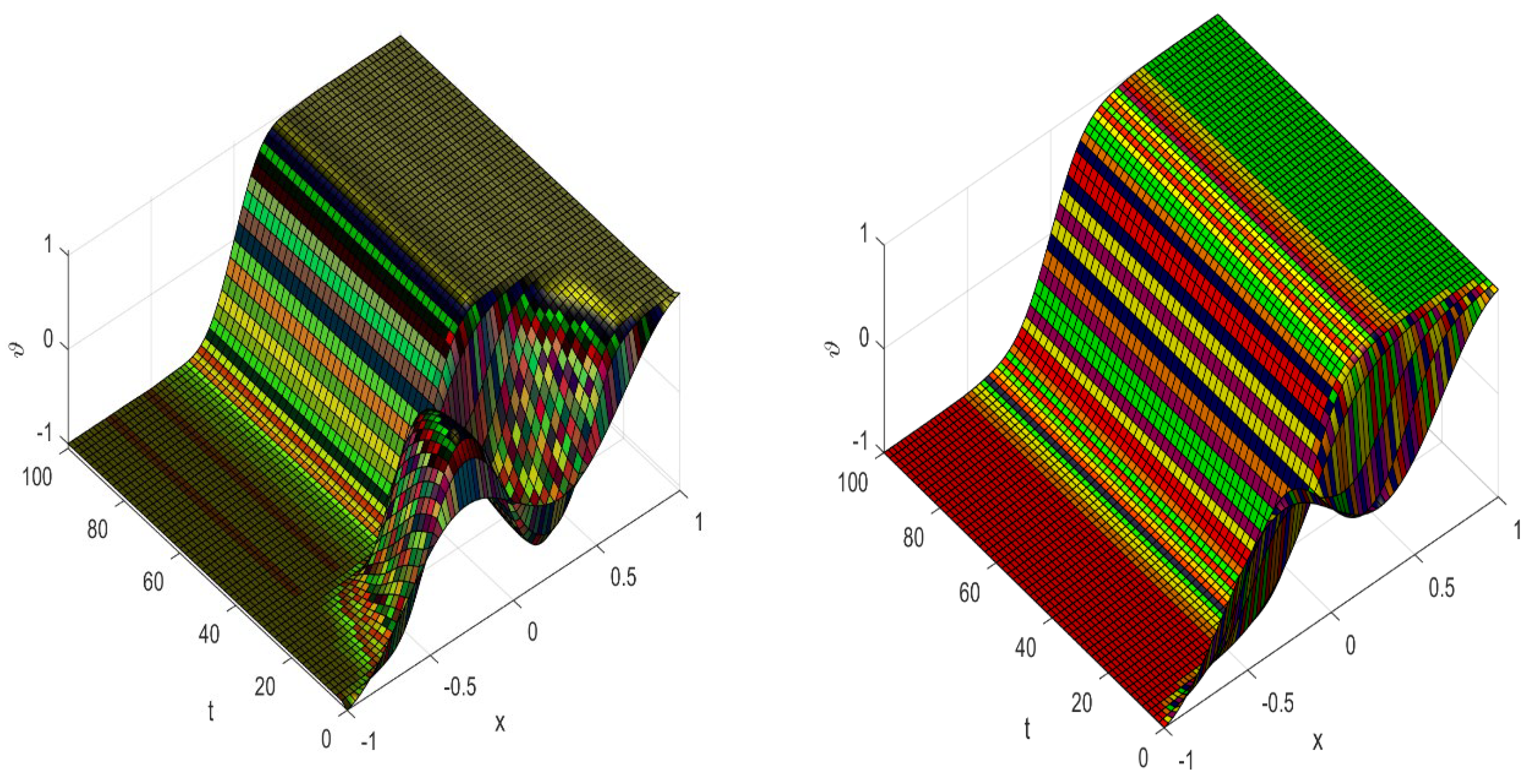
Figure 4,
Figure 5,
Figure 6 and
Figure 7 illustrate the numerical solutions of the KPP-Fisher equation (36) in one, two, and three dimensions. The 1D dynamics show a stable spatiotemporal evolution, as depicted in
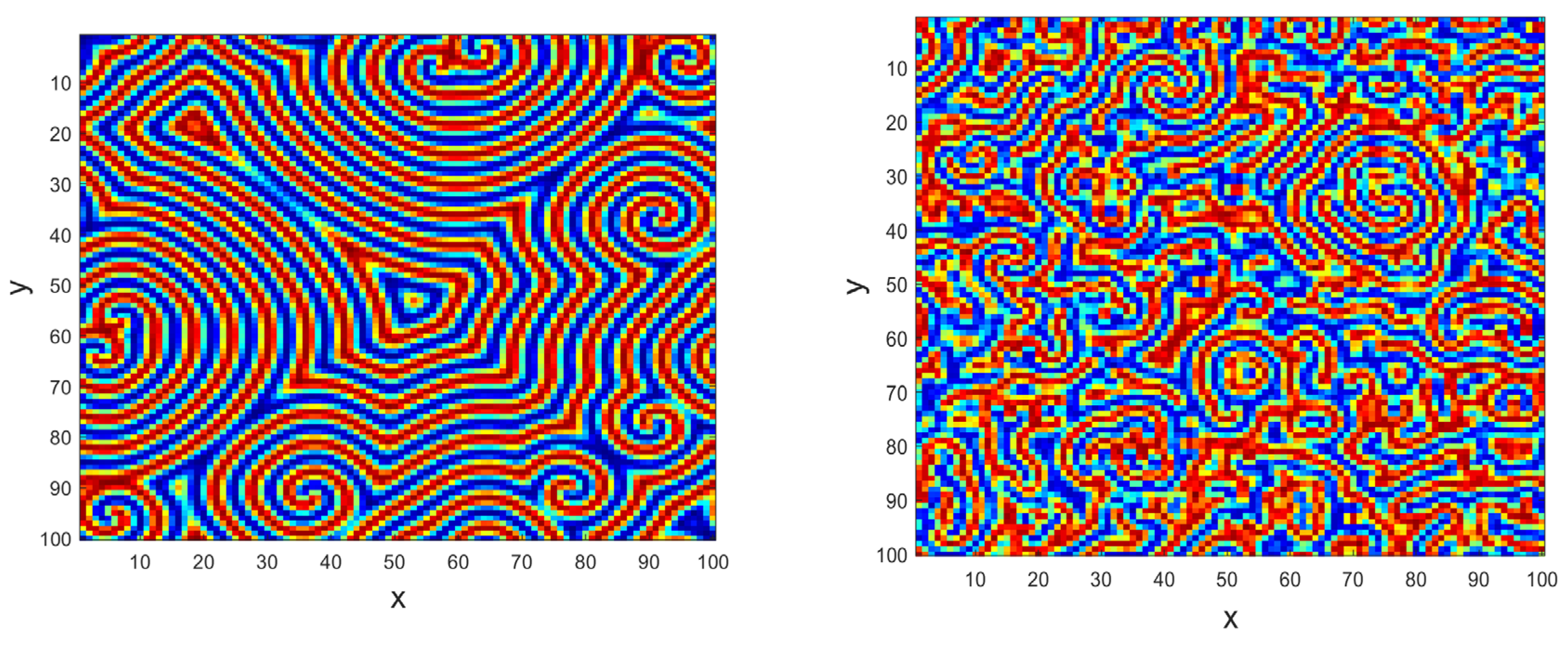
Figure 4 (see caption for details). The 2D dynamics resemble the Allen-Cahn distribution due to similarities between the two equations. Simulations with the initial conditions (41) and (42) produce the results shown in
Figure 5 and
Figure 6, respectively. The complex dynamics of the 3D evolution, starting from the initial condition in (43), are presented in
Figure 7.
The KPP-Fisher equation is a fundamental partial differential equation in mathematics and applied sciences. Its ability to model the spread of populations, genes, or chemical substances makes it a versatile tool in population genetics, ecology, and chemical kinetics. The equation’s traveling wave solutions provide deep insights into how advantageous genes spread through a population, how species expand their habitats, and how chemical reactions propagate through space. Understanding and solving the KPP-Fisher equation continues to be a significant area of research, with applications in various scientific and engineering disciplines.
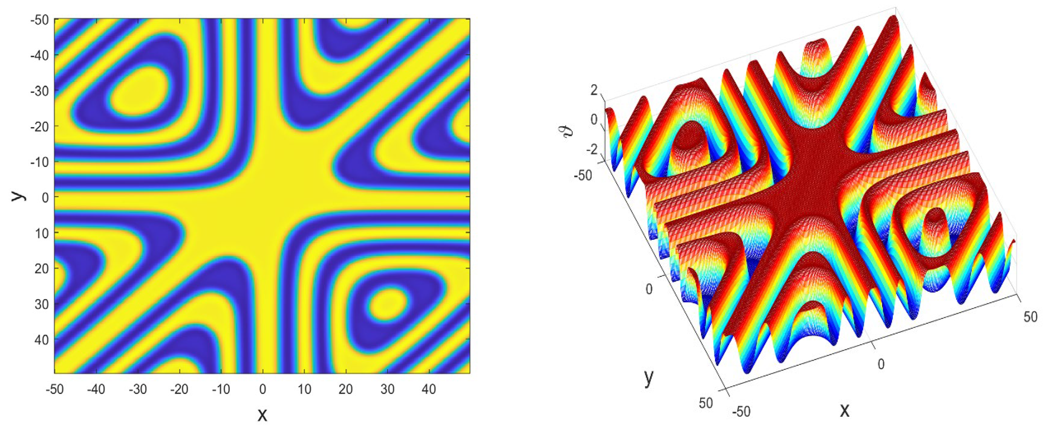
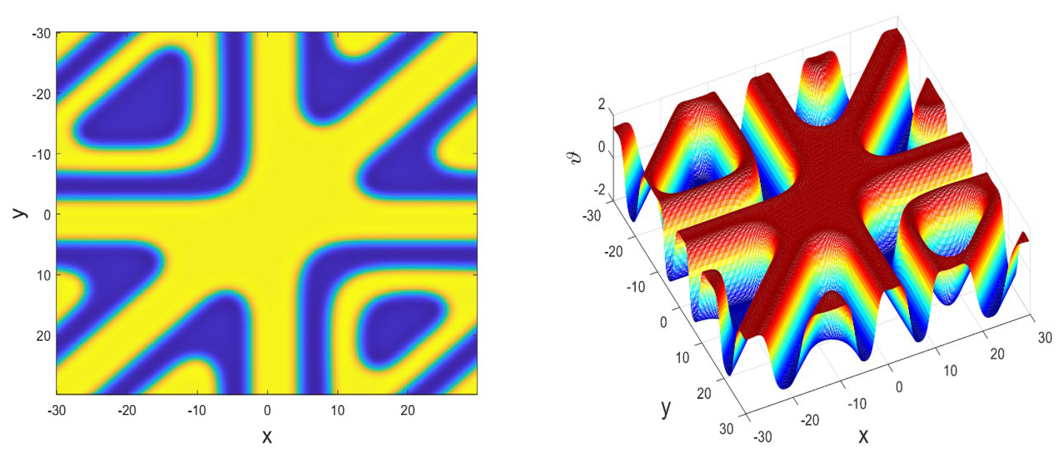
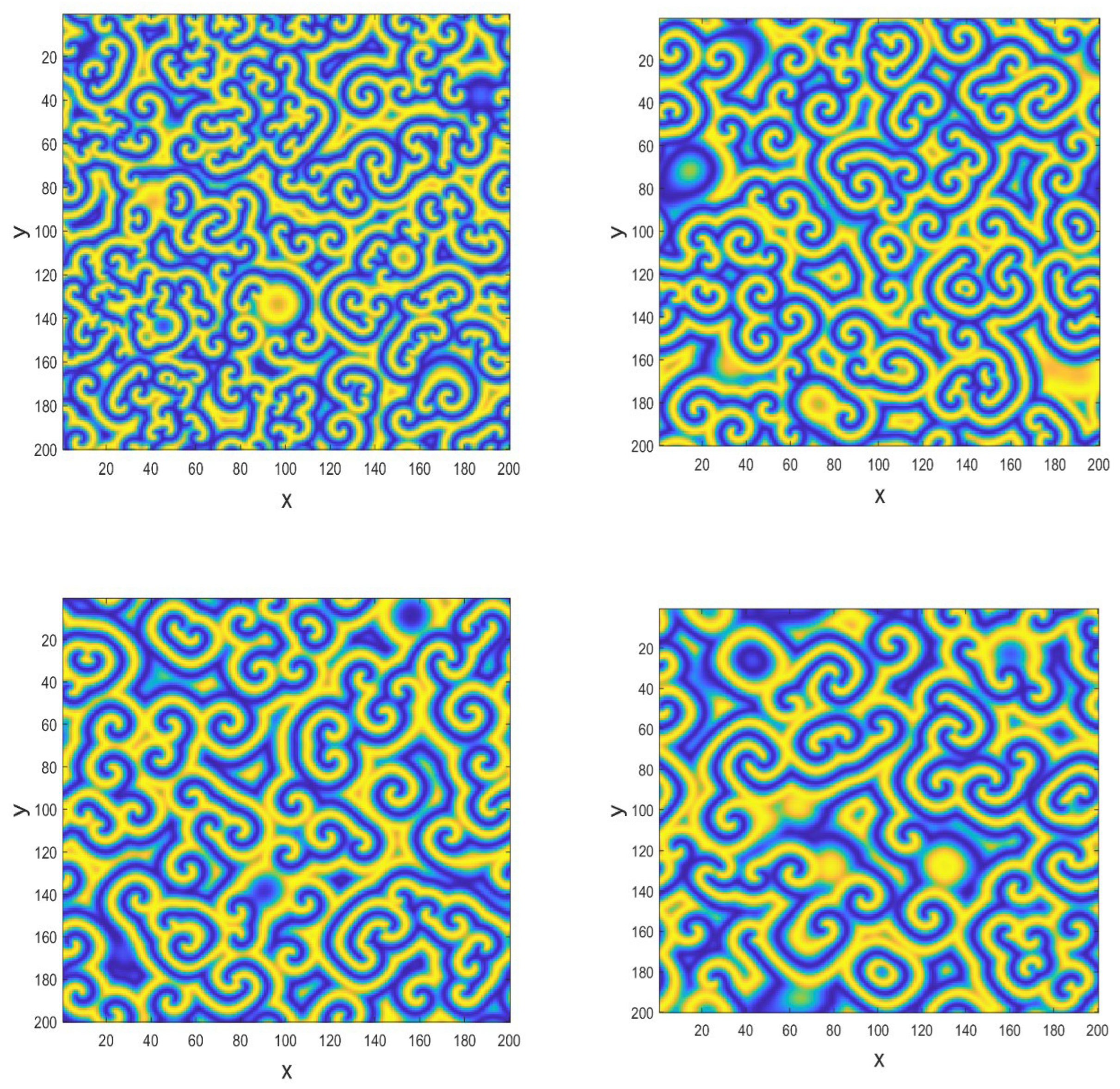
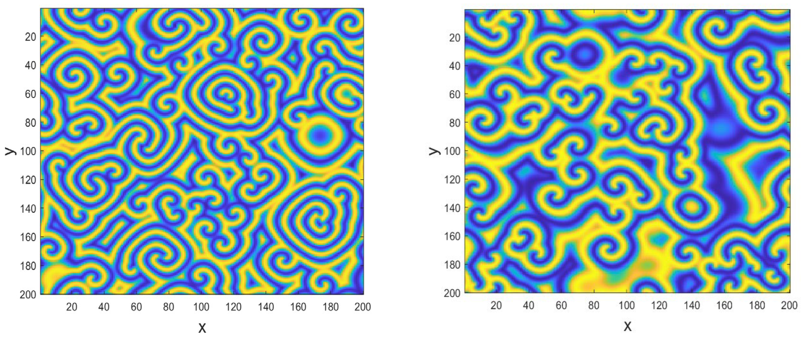
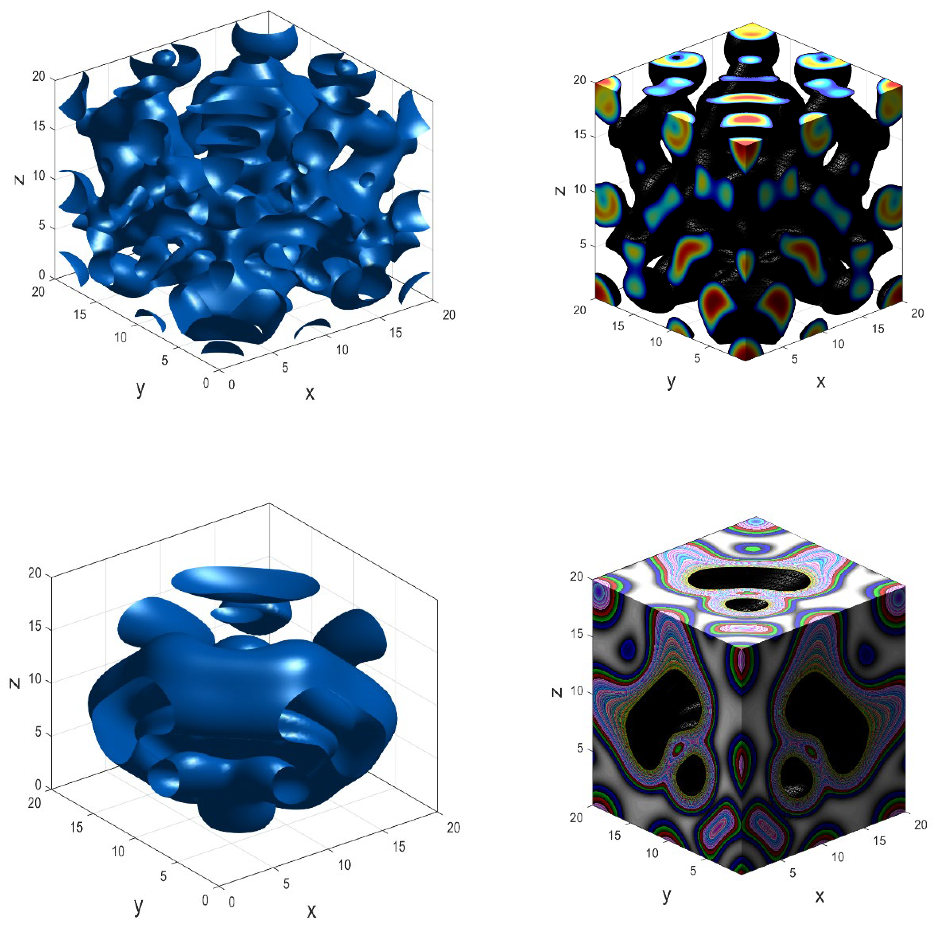
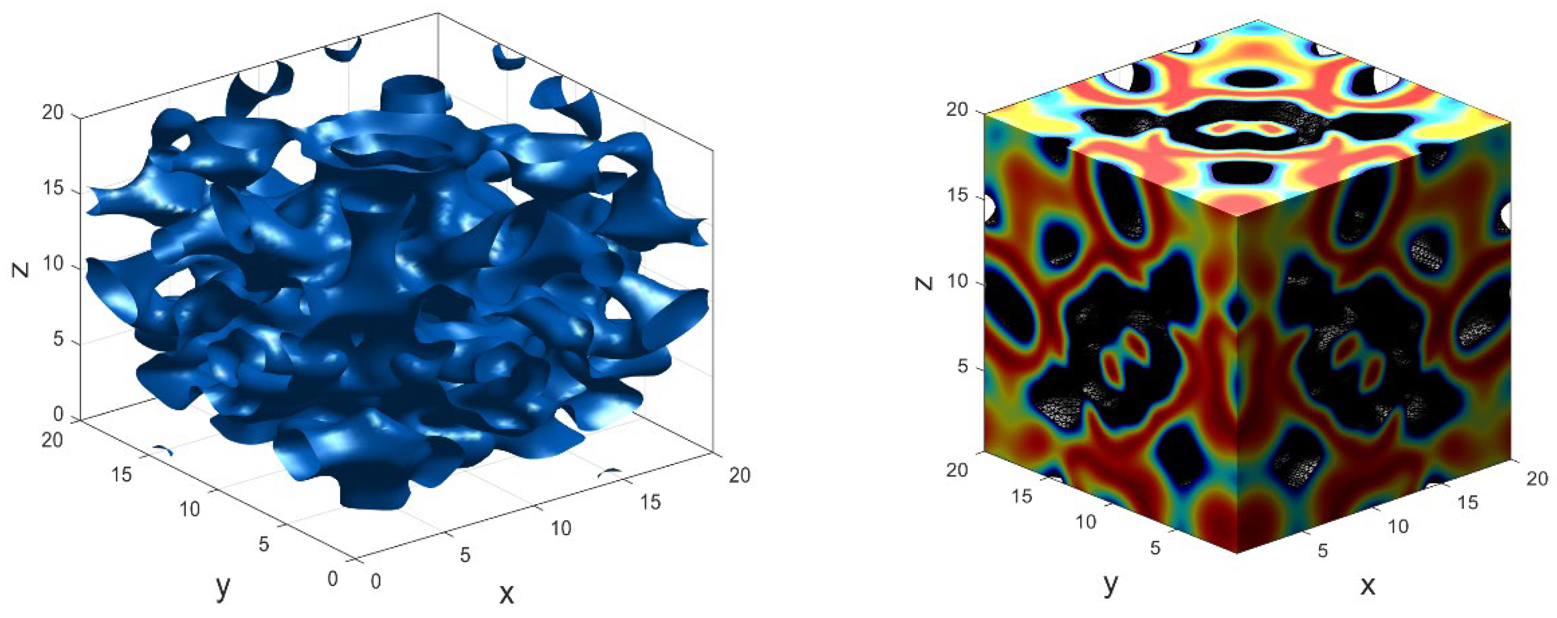
Finally, we present numerical results for fractional complex Ginzburg-Landau (CGL) equation (38) as displayed in
Figure 8,
Figure 9,
Figure 10 and
Figure 11. The CGL equation is known for its oscillatory and spiral distribution behavior, this ie evident in the 2D and 3D dynamics.
The Ginzburg-Landau equation is a cornerstone in the study of nonlinear dynamics and pattern formation as evident
Figure 8,
Figure 9,
Figure 10 and
Figure 11. By describing the evolution of disturbances near a finite wavelength bifurcation, it provides a powerful framework for understanding how complex structures emerge in a variety of physical, chemical, and biological systems. Its applications span numerous fields, making it a versatile and essential tool in both theoretical and applied research.
