Pre-Detection and Pre-Registration Averaging of Full Wave Signals in Airborne LiDAR Bathymetry

Preprint

Technical Note

Pre-Detection and Pre-Registration Averaging of Full Wave Signals in Airborne LiDAR Bathymetry

Altmetrics

Downloads

Views

Comments

A peer-reviewed article of this preprint also exists.

This version is not peer-reviewed

Submitted:

09 September 2024

Posted:

10 September 2024

You are already at the latest version

Alerts

Abstract

A well known technique to enhance the signal to noise ratio (SNR) of repetitive signals is to average them. The coherent parts of the signal add up constructively while the incoherent parts are averaged out. The prerequisite is that the signals are acquired under conditions of high repeatability, i.e.\ the signals must be sufficiently similar. In the present technical note we describe an efficient method for maintaining signal similarity by ensuring spatial and temporal proximity of laser waveform signals obtained by a sensor operated from an airborne platform. The method makes use of a few auxiliary parameters such as laser pulse repetition rate, mirror rotation rate, platform altitude, and flight speed. The method can be extended to be operated in real time.

Keywords:

Subject: Environmental and Earth Sciences - Remote Sensing

1. Introduction

Light in the visible region has the ability to substantially penetrate into water bodies. A common wavelength of laser sources used for bathymetry is 532

n

m

which is visible as green light and is close to the optimum. Light detection and ranging (LiDAR) bathymetry measures the time a pulse of such green light needs to travel from the laser source to an underwater target and back to the instrument’s receiver. Furthermore, the power density is reduced through beam geometry and scattering. As the pulse propagates through air and water it looses energy by interaction with the medium. As a result, the pulse amplitude at the receiver can become very weak, i.e. the signal-to-noise ratio (SNR) becomes very small, which can make reliable detection of the ground difficult.

One conceivable remedy to make the pulse stronger at the receiver would be to increase transmission power. Alternatively another method is to try to reduce the noise. On the one hand, it is conceivable to further improve the optical and electronic components, such as narrower optical filters and amplifiers that contribute very little noise. On the other hand storing the received signal samples, a.k.a Full-Waveform, enables SNR enhancement during post-processing.

Gutierrez et al. [1] mention the possibility of sensitivity enhancement by "averaging multiple waveforms over homogeneous surfaces" and call this stacking. Stacking generally refers to methods of averaging a number of measurements in order to enhance the coherent parts and attenuate the noise, thereby increasing the SNR. For a review of the history of stacking as used in seismic exploration see Rashed [2]. Stacking methods already have been successfully used in LiDAR by Stilla et al. [3] who describe a method of how to automatically align neighboring waveforms in order to maximize coherency and detect weak pulses. They assume a plane geometric structure in the local neighborhood and sweep over a range of angles until a maximum is found. Mader et al. [4] use waveform-stacking in LiDAR bathymetry. They use the water surface as the prominent geometric feature to align the single waveforms before averaging. For mainly horizontal ground geometries, they find that the recognisability of ground points is actually improved. It appears noteworthy, that they do not directly use the stacked waveforms for estimation of the resulting target distances, but use the distance found from the stacked waveform to define a search range within which the final range is estimated from the single waveform.

Averaging, which is at the core of waveform-stacking, has a long history in remote sensing. Motivated by a work of Lee et al. [5], George and Zamanakos [6] investigated so called Comb Filters for enhancement of SNR in Radar. Comb filters result from coherently adding up a periodic signal and can be implemented as a tapped delay line. This type of signal processing was called pre-detection averaging because the summation of the repeated pulses, taking into account the phase of the echo signal, takes place before signal detection [see e.g., [7]].

In LiDAR with the advent of digital signal processing it became feasible to record the output signal of the optical detector. The coherent addition of several such signals before processing, i.e. detecting targets, is another closely related form of pre-detection averaging and has been used by Riegl [8] and Pfennigbauer et al. [9] for some time.

In this technical note we will describe an efficient variant of pre-detection averaging that can be applied to full-wave laser data and discuss it specifically for use in bathymetry. In section 2 we describe the data sets used for the assessment and explain the algorithms. In section 3 we present the results and discuss them in section 4. We conclude with section 5.

2. Materials and Methods

2.1. Datasets

We used four data sets, two from the French Mediterranean coast covering the same area but flown with different parameters, a third from the Venetian lagoon and the fourth from the Venetian Porto di Lido - Canale di Nicolò (PdLCdN). Key parameters are listed in Table 1. The area at the French Coast was flown twice, with different pulse repetition rate (PRR) settings. The set with

PRR = 200 kHz

has been further grouped into two subsets because of the different ground speeds, the G1 set being closer to the shore. The datasets of Venice were recorded on 1st June 2024, the French data set on 19th December 2023. The latter was recorded from an uncrewed platform at a much lower flight speed. Swath and altitude data have been calculated from online waveform processing (OWP) laser range results and off nadir angles from trajectory data. Point density is a nominal value in the center of the swath, of either the forward or backward looking direction only. Swath width, however, only is a first order approximation based on an average off-nadir angle, not addressing the ellipsoidal distortion of the scan pattern. The nominal value of mirror rotation speed was the same for all sets.

Although no data on water turbidity for the Venice Lagoon was collected during the survey, a value of 4 FNU to 7

FNU

1 at the day of data acquisition can be found from satellite observations using the European Union-Copernicus Marine Service [12] which is given, however, outside the lagoon. At the day of acquisition of the French datasets no value is available from European Union-Copernicus Marine Service [12], but at 25th December 2023 a reading of 0.6

FNU

and at 15th December 2023 a reading of 0.3

FNU

is available from the same service.

2.2. Sensor

All Datasets have been acquired by sensors of type VQ-840-G from company Riegl [13]. This sensor type is a compact topo-bathymetric laser scanner for airborne platforms with OWP and full waveform recording for full waveform analysis (FWA) in post processing. The recording is unconditional, i.e., no trigger condition depending on presence of a target is required to initiate the acquisition of data-samples. This is an essential prerequisite for using the method described in this technical note, as the signal before averaging may be too small to trigger the recording.

The laser wavelength of the instrument is in the green at 532

n

m

with a selectable beam divergence and receiver field of view. The scanner is equipped with a rotating mirror that is arranged in such a way that the nadir angle of the resulting laser beam has little variation over a scan line. The effective scan-pattern is nearly elliptic with an off-nadir angle of ±20

°

perpendicular to flight direction and ±14

°

in flight direction. The pulse repetition rate is selectable between 50

kHz

and 200

kHz

while the angular rotation of the mirror is between 10 and 100 lines per second.

The sensor has also been equipped with internal inertial measurement unit and global navigation satellite system (IMU/GNSS) unit.

2.3. Pre-Detection Averaging

If a number of received signals

\begin{matrix} \begin{matrix} r_{i} (t) = p (t) + n_{i} (t) \end{matrix} \end{matrix}

(1)

are modeled as disturbed by additive white Gaussian noise (AWGN) with

\begin{matrix} \begin{matrix} E {n_{i} (t)} & = 0 and & E {n_{i} (t) n_{j} (t)} & = \{\begin{matrix} 0 & i \neq j \\ σ^{2} (t) & i = j \end{matrix}, \end{matrix} \end{matrix}

(2)

the pre-detection averaging estimator

\hat{p} (t)

p (t)

is defined by

\begin{matrix} \begin{matrix} \hat{p} (t) = \frac{1}{N} \sum_{i = 0}^{N - 1} r_{i} (t) \end{matrix} \end{matrix}

(3)

which has a smaller variance than estimating

p (t)

by a single instance of

r_{i} (t)

. The second order statistical properties of this estimator are

\begin{matrix} \begin{matrix} E {\hat{p} (t)} = p (t) \end{matrix} \end{matrix}

(4)

for the expected value and

\begin{matrix} \begin{matrix} E {{(\hat{p} (t)) - p (t))}^{2}} = \frac{1}{N} σ^{2} (t), \end{matrix} \end{matrix}

(5)

for the variance, which is reduced by the factor N, the number of averaged signals. The SNR, a measure of statistical significance, is given by

\begin{matrix} \begin{matrix} SNR (t) = \frac{| E {\hat{p} (t)} |}{\sqrt{E {{(\hat{p} (t)) - p (t))}^{2}}}} = \sqrt{N} \frac{| p (t) |}{σ} \end{matrix} \end{matrix}

(6)

and can be seen to increase proportional to the square root of the number of averaged signals.

2.4. Depth Performance

Maximum depth measurable with LiDAR depends on water turbidity. The secchi-depth

Z_{s}

as standardized in ISO 7027-2 [11] is defined as "the depth at which a matt, circular disc no longer is visible". The method, although not providing an exact measure of water clarity, since influenced by environmental factors, e.g., sun’s glare and operators eyesight capabilities, is a commonly used gauge for illustrative indication of performance in laser bathymetry.

The signal power at the receiver

P_{r}

, reflected from the water bottom at depth z, follows an exponential law

\begin{matrix} \begin{matrix} P_{r} = P_{t} κ e^{- 2 γ z} \end{matrix} \end{matrix}

(7)

with transmitted peak power

P_{t}

, system factor

κ

, and attenuation

γ

. The attenuation factor

γ

and the secchi-depth

Z_{s}

are related by

\begin{matrix} \begin{matrix} γ Z_{s} = η \end{matrix} \end{matrix}

(8)

where

η

is reported in the range 1.1 to 1.7 by Guenther [14], 1.7 to 2.3 in ISO 7027-2 [11], or 1.48 in a recent publication by Lee et al. [15].

Assuming the minimum SNR required to detect a target at depth z is

\begin{matrix} \begin{matrix} SNR = \frac{P_{t} κ e^{- 2 γ z}}{σ}, \end{matrix} \end{matrix}

(9)

to detect a target at

z + Δ z

the following equation can be established by using Equation (6)

\begin{matrix} \begin{matrix} \frac{P_{t} κ e^{- 2 γ z}}{σ} = \sqrt{N} \frac{P_{t} κ e^{- 2 γ (z + Δ z)}}{σ} . \end{matrix} \end{matrix}

(10)

Canceling common factors on both sides the following expression can be obtained indicating the expected averaging count N required to increase the resolvable depth by

Δ z

\begin{matrix} \begin{matrix} N = e^{4 η \frac{Δ z}{Z_{s}}} . \end{matrix} \end{matrix}

(11)

2.5. Coherence Enhancement

Equation (1) is applicable in a strict sense only as a model of a laser echo signal in a non scanning situation. In a scanning situation every

r_{i} (t)

will be a received signal from a different position and direction of the laser beam. Consequently Equation (1) must be changed to

\begin{matrix} \begin{matrix} r_{i} (t) = p (t) + Δ p_{i} (t) + n_{i} (t) \end{matrix} \end{matrix}

(12)

where it is assumed, that the

Δ p_{i} (t)

are deterministic differences caused by the difference in target geometries due to scanning.

Δ p_{i} (t)

is zero for the one measurement treated as reference. In consequence estimator (3) becomes biased

\begin{matrix} \begin{matrix} E {\hat{p} (t)} = p (t) + b (t), \end{matrix} \end{matrix}

(13)

with bias

\begin{matrix} \begin{matrix} b (t) = \frac{1}{N} \sum_{i = 1}^{N - 1} Δ p_{i} (t) . \end{matrix} \end{matrix}

(14)

The variance of the estimator is biased too, viz

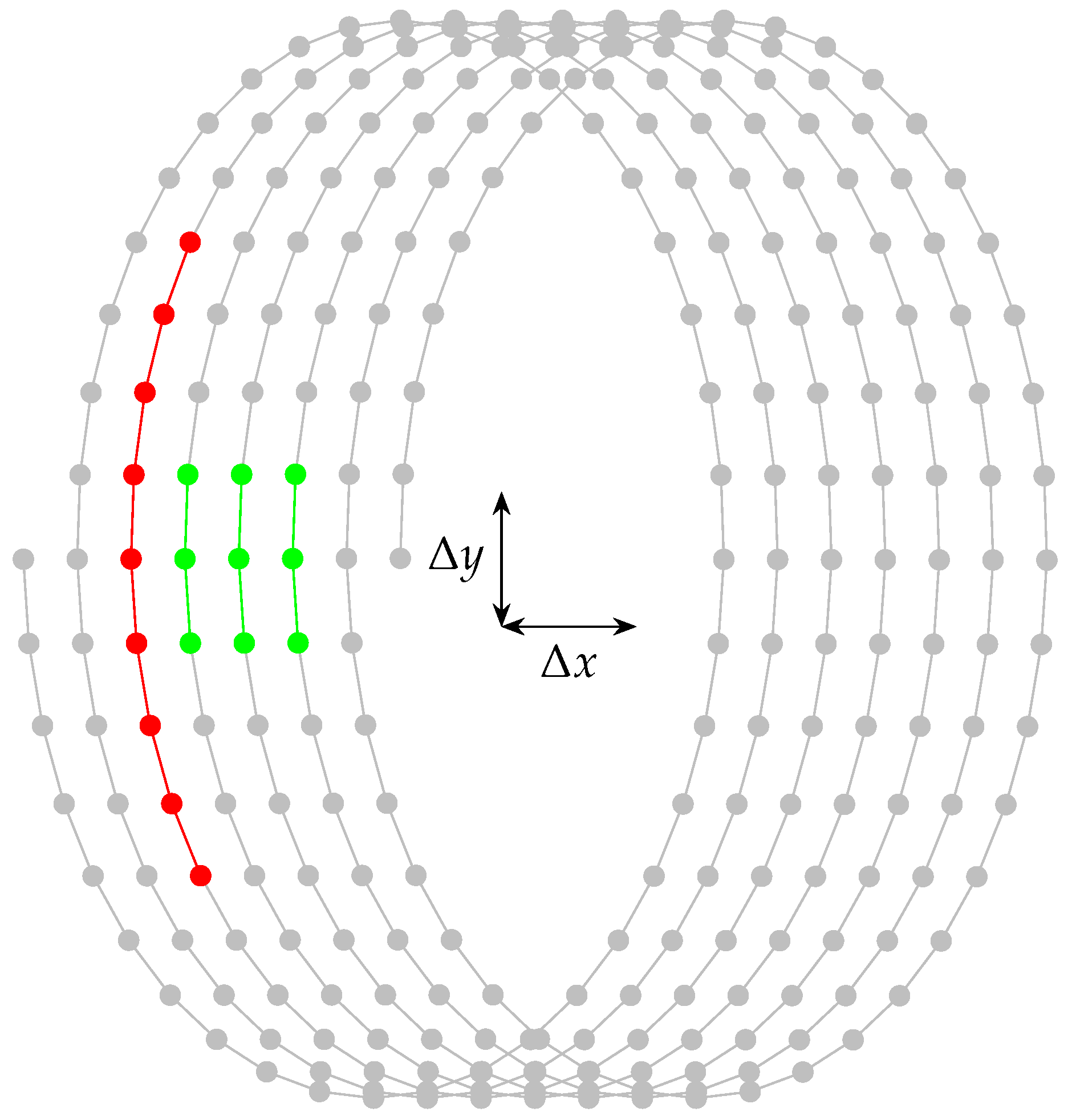
\begin{matrix} \begin{matrix} E {{({\hat{p}}_{i} (t)) - p (t))}^{2}} = b^{2} (t) + \frac{1}{N} σ^{2} (t) . \end{matrix} \end{matrix}

(15)

Enhancing coherence for a scanning instrument operated on a moving platform means reducing the bias by making the laser beam origins as close and their directions as parallel as possible. The circular scan pattern of Figure 1 is typical for bathymetric scanners for it allows to approach an almost constant nadir angle of the beam. Incremental movement

Δ x

of the platform is superimposed with an incremental rotation

Δ y

of the laser deflection mechanism. A number of adjacent shots, although close in time, can be spread out spatially quite substantially, as is indicated by the red points in Figure 1. For the same number of laser shots, the maximum spatial extent is reduced by the grouping of shots not only in time but also in space. The green dots in Figure 1 illustrate the idea.

The optimal number of lines

n_{x}

and shots

n_{y}

for a given averaging number is determined by searching for factors

n_{x}

and

n_{y}

such that

n_{x} Δ x \approx n_{y} Δ y

while keeping the product

n_{x} n_{y}

close to the given averaging number. For post-processing the required values

Δ x

and

Δ y

can be obtained from the flight trajectory and measurement data by

\begin{matrix} Δ y = r sin (θ) Δ ϕ = r sin (θ) \frac{ω}{PRR} \\ Δ x = v \frac{2 π}{ω}, \end{matrix}

(16)

with r the average distance to the water surface,

θ

the nadir angle,

Δ ϕ

the angular shot increment, v the speed of the platform, and

ω

the angular rotation speed of the scan mechanism.

Δ ϕ

is related to

ω

by the PRR. As this data is also available during the flight, i.e. prior to point cloud registration, the method described in this note can in principle also be carried out in real-time. To be precise, Equation 16 is only exact for a circular scan pattern and even then only in the center of the swath. Nevertheless, we use it as a first order approximation.

In general, the times of flight of two echo pulses that occur at different beam angles on an inclined plane are unequal. While in theory the beam angles with respect to a horizontal water surface or a horizontal water bottom should be the same for different shots in a quasi circular pattern as in Figure 1, this is not the case in practice. Pitch and roll angles of the platform as well as non-horizontal ground cause deviations from the ideal situation, and thus different times of flight.

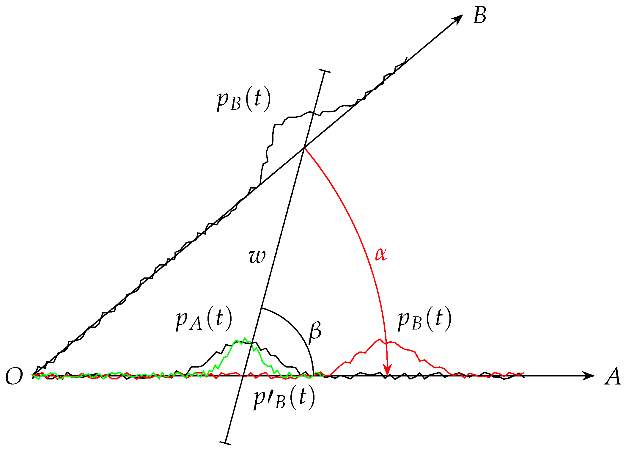
Figure 2 shows the general case. Two echos from laser beams A and B, enclosing angle

α

, are reflected from a slanted plane w with the angle

β

w.r.t. beam direction

O - A

. Assuming that the velocity in direction of flight is small enough so that the platform does not move much between successive laser shots, a fixed point O is used for both beams. Neglecting pulse spreading due to beam divergence and incidence angles on the plane, the two echoes will be of similar shape. If both angles are known the pulse from beam B can be stretched by scaling

\begin{matrix} \begin{matrix} {p^{'}}_{B} (t) = p_{B} (t \frac{sin (β - α)}{sin (β)}), \end{matrix} \end{matrix}

(17)

aligning the pulse location with pulse

p_{A} (t)

at the cost of shape distortion. Differently to Stilla et al. [3], who perform a search for the optimum angle

β

which maximizes coherence, we rely on the angle

α

being small. The same grouping criterion, which guarantees spatial proximity of the laser shots and was explained above, also leads to approximately parallel beams and thus small angles

α

The horizon of the measuring platform is known, as are the angles

α

, thus it is possible to correct the pulse scales for special planes such as the water surface or the ground. We omitted such correction, however, based on the following consideration. A first order Taylor approximation of Equation (17) for small

α

\begin{matrix} \begin{matrix} {p^{'}}_{B} (t) = p_{B} (t (1 - α cot (β))) \end{matrix} \end{matrix}

(18)

reveals that the relative stretching error is proportional to

α cot (β)

. For

β = 90^{\circ}

the error vanishes and for

β = 45^{\circ} to 135^{\circ}

the

| cot (β) |

is smaller than

1.0

meaning for angles

α < \pm 1^{\circ}

the relative error will be 1.7% at most.

2.6. Sliding Buffers

Processing starts by splitting the data of each flight strip from the quasi-circular scan pattern in Figure 1 into two partial strips, one strip in the forward direction and one strip in the backward direction. The splitting defines scan lines: A scan line comprises the laser shots from one edge of the swath to the other. Each of the two sub strips is then processed separately so that the beam directions of neighboring laser shots are approximately the same, ensuring the small angle

α

condition stated in the previous section.

With the number of lines

n_{x}

and the number of shots

n_{y}

used for an averaged waveform, the total number of scan lines held in memory at any one time need never be larger than

n_{x}

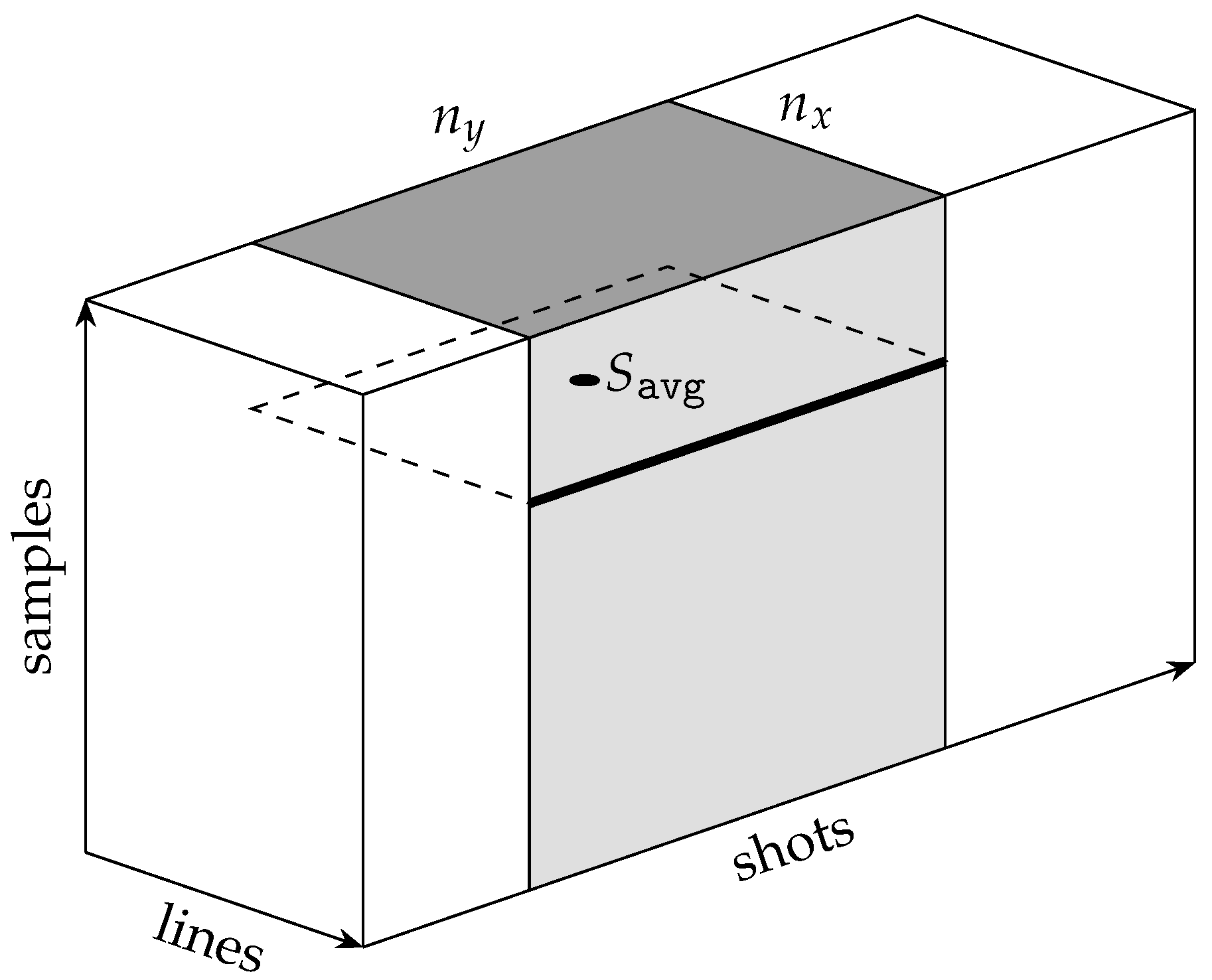
The data of the full waveforms is loaded into a buffer structure for processing which can be addressed via the line number, the shot number, and the sample index as sketched in Figure 3. A batch of

n_{x}

lines is loaded for a processing cycle. After processing a batch of lines, the buffer space of the oldest line can be reused when loading the next line, as the data of the oldest is no longer needed. A simple copy operation is not sufficient, however, for the sample values as they must be brought into a common time grid before averaging can take place. We use a simple linear interpolation scheme for this task but other more sophisticated methods such as, e.g., bandlimited interpolation are possible.

All sample values indicated by the dashed rectangle in Figure 3 contribute to an averaged sample

S_{avg}

. We do not, however, perform a plain averaging operation, but also do an outlier removal which effectively removes spurious samples that can occur as a result of the very sensitive sensor.

A cycle of the averaging process then runs in such a way that all lines of the outer cuboid are loaded in which the gray sub-cube then slides along the shot axis and at each position of the gray sub-cuboid the innermost rectangle slides over all samples. The process continues with the next cycle by loading the data of the next line until all lines have been processed.

The total number of averaged waveforms will thus be close to the number of raw waveforms. A small difference results because at both ends of the swaths from the forward and backward looking sub-strips no averaging is possible.

2.7. Bathymetry Map and Image Preparation

The averaged waveforms were analyzed using the Surface Volume Bottom (SVB) algorithm by Schwarz et al. [16] and converted into a globally registered point cloud. After classification of the water surface points a water surface model was created and used to apply refraction correction to the underwater points. The classification of the bathymetric points in the turbid Venetian datasets was done manually. The classification of the bathymetric points from the French datasets was done by using a depth threshold to cut off the water surface followed by some manual corrections.

RiProcess from company Riegl [17] was used for averaging, SVB analysis, and refraction correction, while the free software tool QGIS [18] was used for map preparation and 3D visualization.

3. Results

The nominal averaging count for post processing of all sites has been set to 100. The criterion for obtaining a shape as square as possible led to virtual spot diameters of

\approx 1.2 m to 2.2 m

for the French data sets and ≈ 8.8 m to 9.2

m

for the Italian datasets. The virtual diameter is the sum of of the intrinsic spot size and the diagonal’s length of the averaged area. The smaller virtual spot size of the French datasets is due to a a higher point density resulting from the slower airspeed of the uncrewed platform. A summary of parameters is given in Table 2. N is given by the product

n_{x} \times n_{y}

and the averaged area is

n_{x} Δ x \times n_{y} Δ y

. It can be seen that the averaged area always is almost square despite different point densities in flight and across directions.

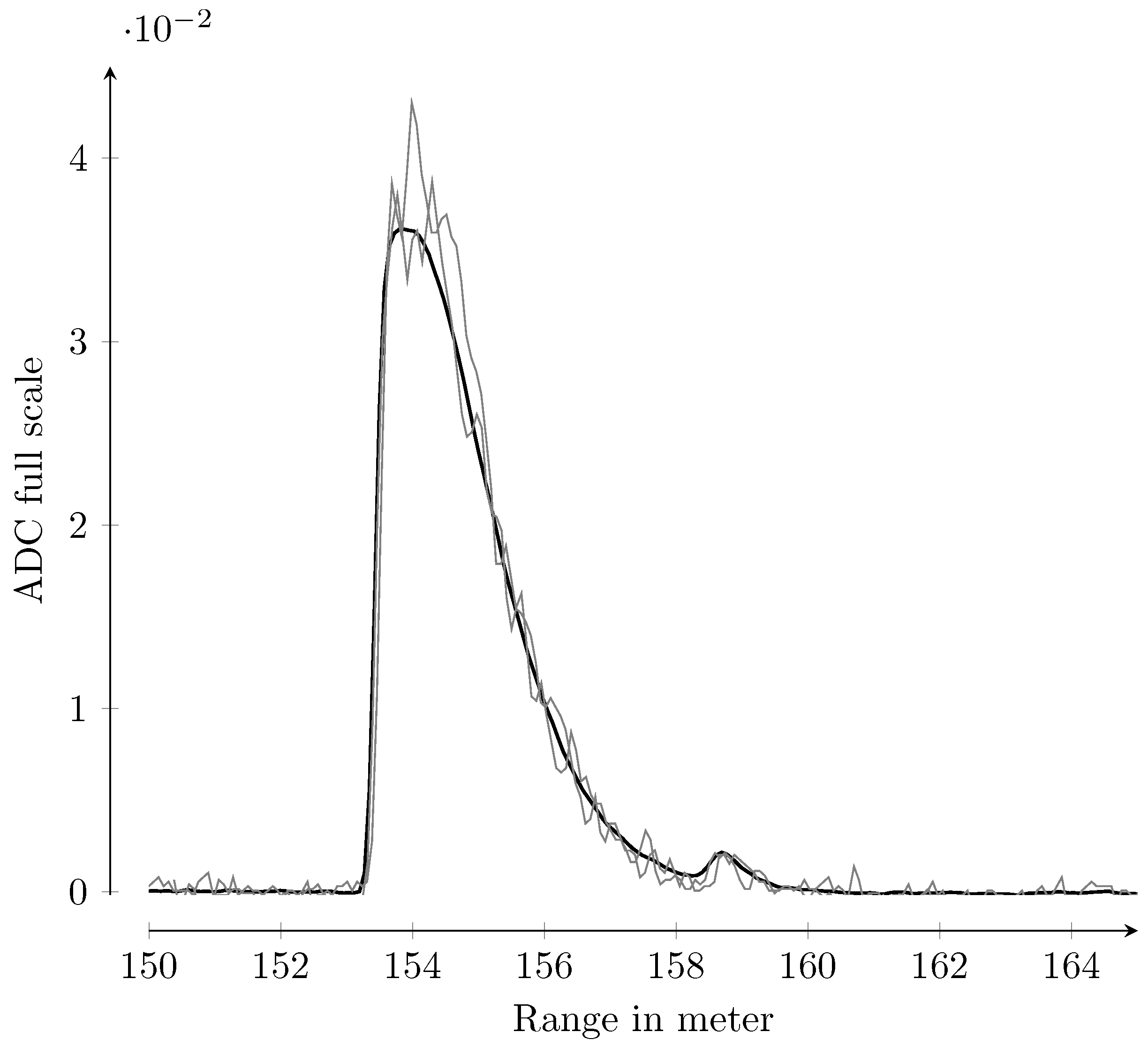
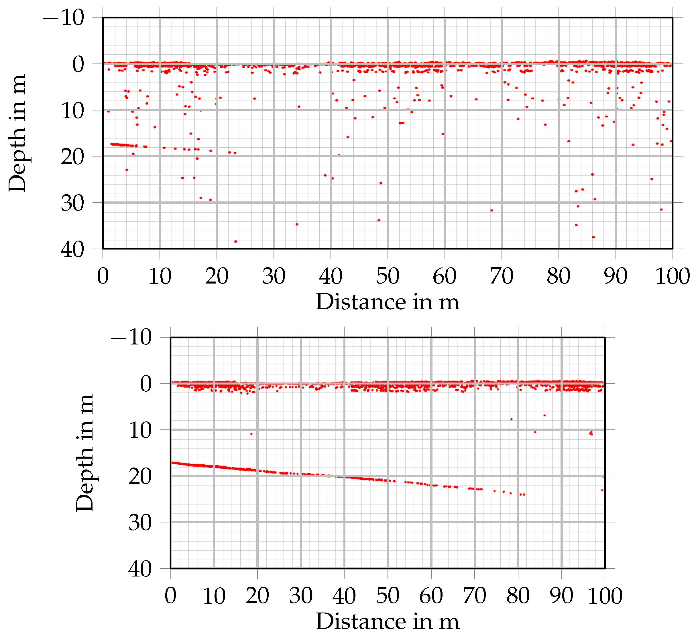
The effectiveness of pre-detection averaging is demonstrated in Figure 4 and Figure 5. Figure 4 showing two randomly selected pulses from the neighborhood of a shot, in thin gray, and the average of ≈ 100 surrounding pulses, in solid black. The averaged pulse is of smoother shape with a much lower number of local extrema. The numbers of averaged pulses, however, is only approximate for two reasons: first because the actual number is subject to the squareness criterion as described in section 2.5, second because outliers are removed prior to averaging.

For Figure 5 two profiles from France 2 dataset have been taken at the same crosscut location. The upper profile is without averaging, while the lower profile has been created using an effective averaging number of

N = 93

. The maximum resolvable depth in the not averaged case is 19

m

and 24

m

with averaging. The improvement due to averaging thus is 5

m

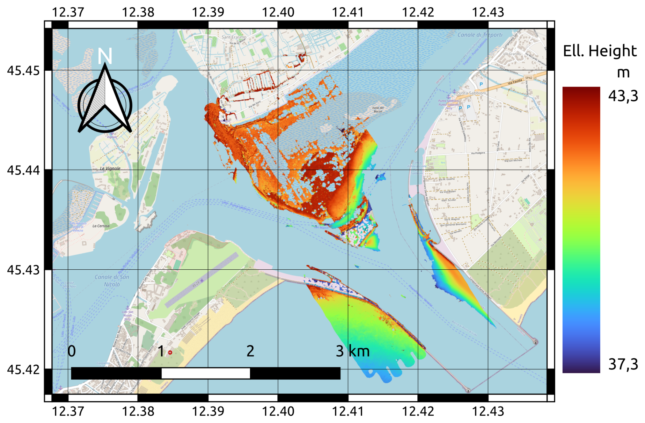
Although turbidity in the Venice area was high, underwater points could be determined from all three areas surveyed. Figure 6 shows a map of Porto di Lido - Canale di Nicolò superimposed with bathymetric points mapped to color. The maximum penetration depth of the laser below the water surface was about 6

m

on the day of recording. The underwater structures of the MOSE (Modulo Sperimentale Elettromeccanicao), the Venetian flood protection system, are not visible in the bathymetry because when it is not in operation its parts lie below the penetration depth of the laser.

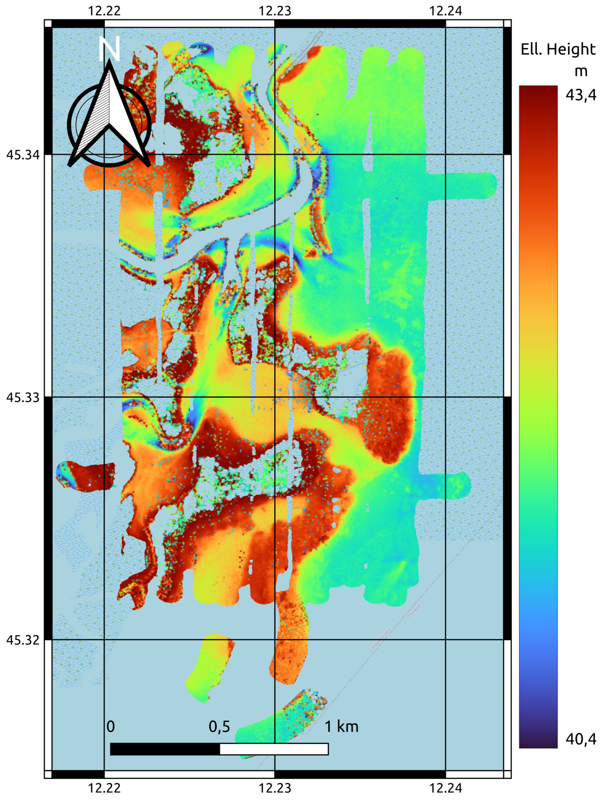
Maximum penetration depth within the Venetian Lagoon was similar to that of the PdLCdN dataset, the color map, however, has been set to cover 3

m

only to emphasize the high capability of structure resolution in the shallow water. Figure 7 exhibits a map of underwater bathymetry of the surveyed area. Some voids visible in north south direction are due to insufficient overlapping of flight strips. The map consists of bathymetric underwater points only and shows noisy gaps in places where land cover would be expected, as the model of the SVB algorithm is only suitable for underwater analysis. No maps for comparison purposes could be created without prior averaging of the datasets, because classification of bathymetric points was severely hindered by the large amount of spurious points in that case.

Turbidity was very low at the French Mediterranean Coast and the data showed that a depth penetration of 24

m

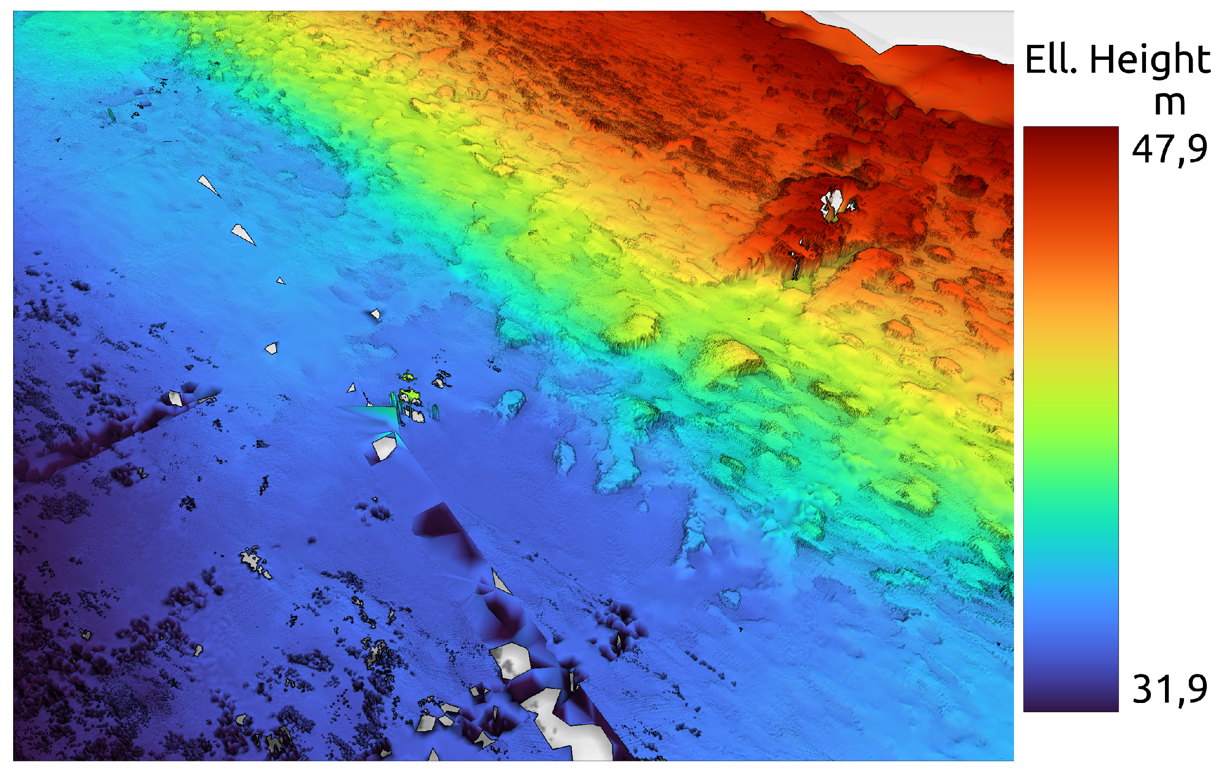
could be attained. Figure 8 shows a detail view of the water bottom in perspective projection, taken from the France 1 G1 dataset, highlighting that it is possible to obtain structures in high resolution despite a high averaging number provided flight conditions are appropriate. The rocks in the centre axis of the picture are of diameter approx. 6

m

. The visual appearance of the rocks has been further enhanced by applying a shadowing effect. Maximum depth could not be achieved in the France 1 dataset, because of a storage limitation that applies for long waveform recordings taken with a setting of 200

kHz

for the PRR.

4. Discussion

The effect of summation of a group of closely spaced laser beams with small footprint can be understood as being equivalent to a single pulse with a larger footprint. It is known, e.g., that proper selection of beam divergence, and thus footprint size, can be used to compensate for the influence of surface waves using the averaging effect over the footprint size [see. e.g. 14]. Although the purpose of averaging is different in that case, the principle is the same, which in our opinion justifies the name virtual footprint caused by the group of laser beams subjected to averaging.

As has been stated in section 2.4, the improvement in depth penetration should be logarithmic in the number of averaged waveforms.

\begin{matrix} \begin{matrix} Δ z & = \frac{ln N}{4 η} Z_{s} i . e ., & 5 m & \approx \frac{ln 93}{4 \times 2.15} \times 9.5 m . \end{matrix} \end{matrix}

(19)

From experience [19] we learned that typically two times the Secchi depth can be reached with the particular sensor type with SVB waveform processing. In an attempt to compare the theoretical relations with the empirical findings without having available on-site measurements of Secchi depth, we use the top profile in Figure 5, where a maximum depth penetration of 19

m

is achieved, to estimate

Z_{s}

to be 9.5

m

. Furthermore, a value of 2.15 for

η

is taken in accordance with ISO 7027-2 [11]. With these values relation (19) is met quite closely.

One of the adverse effects of averaging is, as must be expected, a reduction in resolution of the target scene due to the low pass behavior of averaging. This effect, however, depends on the sampling parameters of the un-averaged dataset as can bee seen in Figure 8. The strong oversampling in the France 1 G1 dataset still allows a high averaging rate without compromising resolution. But even if resolution is reduced a certain degree of averaging will be highly beneficial because robustness against the influence of surface waves is increased, thus improving derivation of the water surface. Theoretically, a low pass filtered dataset should be able to be represented with less data without loosing information, as stated by the Nyquist-Shannon sampling theorem. We took, however, the approach of not reducing the amount of data, since often the higher resolution dataset is required for further processing anyways. On the other hand, since the storage and full waveform processing requirements can be demanding the potential for optional reduction may be interesting for some projects.

Although the virtual footprint size of the Italian datasets is already half the size of satellite based systems, e.g., for ICESat-2 the footprint size is 17

m

[20], the airborne system benefits from tunability of the size and can thus be adapted during post processing. Similar to the approach of Mader et al. [4] one can also combine bathymetry with high averaging and one without averaging to increase the resolution by considering targets close to the smoothed bathymetry only.

Another possibility is to increase depth performance without reducing the resolution by scanning faster and flying slower yielding a higher point density an approach particularly interesting for use with uncrewed platforms. Figure 8 is an example of such a use case.

All test data sets show that the approximate Equation 16 suffices for selecting a suitable group of waveforms for averaging. A more thorough analysis would start at a more accurate description of the laser pattern such as the Palmer Scan, i.e., an elliptical pattern [see 21] or at an even more advanced analysis as done by Li [22] taking care of the deviations from the elliptic shape.

Another question that requires consideration is the determination of the mean distance r used in Equation 16. We use the median value that can be obtained from online range measurements, i.e., before the pre-detection step. This means that although these values represent plausible distances above a water surface, they do not necessarily reflect the distance to a water surface in heterogeneous areas with mixed water and land cover. For the Lagoon dataset a discrepancy between the altitude above the water surface as stated in Table 1 and the surface as obtained from the registered pointcloud, as in Figure 7, was observed, however, the effect was not very large. It is a simple extension to use a nominal, manually specified, altitude instead, but at the expense of non-automatic operation.

We described the method for use in post processing, but an extension that allows averaging during the flight in real time is conceivable. From the parameters needed in Equation 16 everything is in available in real time from the IMU/GNSS unit.

Comparing the presented method to an approach where the waveforms are registered into a geographical frame before averaging we can identify the following: Proper registration requires a sufficient number of points that can be derived before averaging is applied. The fact that two points are close to each other in geo-referenced space does not mean that the laser directions associated with them are parallel, a prerequisite for proper averaging.

It should not go unmentioned that the method allows a high degree of parallelism in processing and at the same time has a relatively small, constant memory requirement. This makes it possible to assign each of the horizontal slices that contribute to the

S_{avg}

point in Figure 3 to a separate CPU for simultaneous processing.

While increasing depth performance is one of the goals of averaging, within the scope of this technical note we could also demonstrate the effect of better structure recognition in shallow water. A higher SNR reduces the amount of spurious points resulting in a cleaner pointcloud which greatly assists point classification as demonstrated by the results of Figure 7 and Figure 6 which would not have been possible with the un-averaged datasets.

5. Conclusions

In this technical note, we describe a variant of waveform stacking, a method for increasing the SNR called pre-detection averaging, which is particularly useful as a pre-processing step of full waveform analysis to derive bathymetry. The higher SNR makes possible higher depth resolution and better point classification due to the smaller amount of spurious points. The presented method is fast, requires only a small and constant amount of memory, can be applied to the unregistered dataset, and can optionally be performed in real-time during flight. The single parameter that needs to be set manually is the degree of averaging. The method can be understood as a means to process the data with a virtual footprint size that is larger than the native footprint size. When done during post processing the optimum averaging size can be tuned for best results without the need for new data acquisition.

Author Contributions

Methodology, software, formal analysis, data curation, writing—original draft, visualization, R. Schwarz; conceptualization, validation, investigation, supervision, project administration, funding acquisition, writing—review and editing, M. Pfennigbauer. All authors have read and agreed to the published version of the manuscript.

Funding

This research received no external funding.

Institutional Review Board Statement

Not applicable.

Data Availability Statement

The raw data of the Venice areas supporting the conclusions of this article will be made available by the authors on request.

Acknowledgments

Full waveform data have been provided by Riegl Research and Defense GmbH. This study has been conducted using European Union-Copernicus Marine Service [12] Information; doi:10.48670/moi-00109. Map data copyrighted OpenstreetMap contributors and available from https://www.openstreetmap.org. We would like to thank the Italian civil air traffic control ENAV, in particular the OPS Venezia Tessera, the OPS Venezia Lido and the OPS Padova for coordinating the flight missions.

Conflicts of Interest

The authors are employees of Riegl Research and Defense, which financed the study.

Abbreviations

The following abbreviations are used in this manuscript:

AWGN	Additive White Gaussian Noise
FNU	Formazin Nephelometric Standard
FWA	Full Wave Analysis
IMU	Inertial Measurement Unit
GNSS	Global Navigation Satellite System
LiDAR	Light Detection and Ranging
LPS	Lines per Second
OWP	Online Waveform Processing
PRR	Pulse Repetition Rate
SNR	Signal to Noise Ratio
SVB	Surface Volume and Bottom

References

Gutierrez, R.; Neuenschwander, A.; Crawford, M. Development of laser waveform digitization for airborne LIDAR topographic mapping instrumentation. Proceedings. 2005 IEEE International Geoscience and Remote Sensing Symposium, 2005. IGARSS ’05. IEEE, 2005. [CrossRef]
Rashed, M. Fifty years of stacking. Acta Geophysica 2014, 62, 505–528. [Google Scholar] [CrossRef]
Stilla, U.; Yao, W.; Jutzi, B. Detection of weak laser pulses by full waveform stacking. The international archives of photogrammetry, remote sensing and spatial information sciences 2007, 36, 25–30. [Google Scholar] [CrossRef]
Mader, D.; Richter, K.; Westfeld, P.; Maas, H.G. Potential of a Non-linear Full-Waveform Stacking Technique in Airborne LiDAR Bathymetry. PFG – Journal of Photogrammetry, Remote Sensing and Geoinformation Science, 2021. [Google Scholar] [CrossRef]
Lee, Y.; Cheatham, T.; Wiesner, J. Application of Correlation Analysis to the Detection of Periodic Signals in Noise. Proceedings of the IRE 1950, 38, 1165–1171. [Google Scholar] [CrossRef]
George, S.F.; Zamanakos, A.S. Comb Filters for Pulsed Radar Use. Proceedings of the IRE 1954, 42, 1159–1165. [Google Scholar] [CrossRef]
Skolnik, M.I. Introduction to radar systems, 2nd ed.; McGraw-Hill Book Co: Singapore, 1981; bibtex: skolnik_introduction_1981. [Google Scholar]
Riegl, J. Eyesafe Laser Rangefinder LASERTAPE FG21. Available online: https://web.archive.org/web/20010415212138/http://www.riegl.com/lasertape/e_fg21.htm (accessed on 4 July 2024).
Pfennigbauer, M.; Ullrich, A.; Schwarz, R. Waveform-averaging airborne laser bathymetry scanner. Laser Radar Technology and Applications XXV; Turner, M.D.; Kamerman, G.W., Eds. SPIE, 2020. [CrossRef]
ISO 7027-1, C.S. Water quality - Determination of turbidity - Part 1: Quantitative methods. Standard ISO 7027-2:2019(E), International Organization for Standardization, 2016.
ISO 7027-2, C.S. Water quality - Determination of turbidity - Part 2: Semi-quantitative methods for the assessment of transparency of waters. Standard ISO 7027-2:2019(E), International Organization for Standardization, 2019.
European Union-Copernicus Marine Service. Mediterranean Sea, Bio-Geo-Chemical, L3, daily observation, 2021. [CrossRef]
Riegl. RIEGL VQ-840-G, Compact Topo-Bathymetric Airborne Laser Scannerwith Online Waveform Processing and Full Waveform Recording. Available online: http://www.riegl.com/uploads/tx_pxpriegldownloads/RIEGL_VQ-840-G_Datasheet_2023-09-11.pdf (accessed on 4 July 2024).
Guenther, G.C. Airborne Laser Hydrography System Design and Performance Factors. NOAA Professional Paper Series, National Ocean Service 1.
Lee, Z.; Shang, S.; Du, K.; Wei, J. Resolving the long-standing puzzles about the observed Secchi depth relationships. Limnology and Oceanography, 63, 2321–2336. [CrossRef]
Schwarz, R.; Mandlburger, G.; Pfennigbauer, M.; Pfeifer, N. Design and evaluation of a full-wave surface and bottom-detection algorithm for LiDAR bathymetry of very shallow waters. ISPRS Journal of Photogrammetry and Remote Sensing 2019, 150, 1–10. [Google Scholar] [CrossRef]
Riegl. RiProcess, Data Processing Software. Available online: http://www.riegl.com/uploads/tx_pxpriegldownloads/RiProcess_Datasheet_2024-02-07.pdf (accessed on 10 July 2024).
QGIS.org. QGIS Geographic Information System. Available online: http://www.qgis.org (accessed on 9 July 2024).
Mandlburger, G.; Pfennigbauer, M.; Schwarz, R.; Pöppl, F. A Decade of Progress in Topo-Bathymetric Laser Scanning Exemplified by the Pielach River Dataset. ISPRS Annals of the Photogrammetry, Remote Sensing and Spatial Information Sciences, X-1/W1-2023, 1123–1130. [CrossRef]
Neumann, T.A.; Martino, A.J.; Markus, T.; Bae, S.; Bock, M.R.; Brenner, A.C.; Brunt, K.M.; Cavanaugh, J.; Fernandes, S.T.; Hancock, D.W.; Harbeck, K.; Lee, J.; Kurtz, N.T.; Luers, P.J.; Luthcke, S.B.; Magruder, L.; Pennington, T.A.; Ramos-Izquierdo, L.; Rebold, T.; Skoog, J.; Thomas, T.C. The Ice, Cloud, and Land Elevation Satellite – 2 mission: A global geolocated photon product derived from the Advanced Topographic Laser Altimeter System. Remote Sensing of Environment, 233, 111325. [CrossRef]
Wehr, A.; Lohr, U. Airborne laser scanning—an introduction and overview. ISPRS Journal of Photogrammetry and Remote Sensing, 54, 68–82. [CrossRef]
Li, Y. Elements of optical and laser beam scanning; Number vol. no. 331 in SPIE PM, SPIE Press, 2021. Literaturangaben.

1	$FNU$ is the Formazin Nephelometric Unit [see [10,11]]

Figure 1. Quasi circular scan pattern of a LiDAR bathymetry scanner. Flight direction is in

Δ x

direction, beam rotation in

Δ y

direction (at least in the center of the swatch). The same number of adjacent laser shots (red) make for a smaller virtual spot size if distributed between shots and lines (green).

Figure 1. Quasi circular scan pattern of a LiDAR bathymetry scanner. Flight direction is in

Δ x

direction, beam rotation in

Δ y

direction (at least in the center of the swatch). The same number of adjacent laser shots (red) make for a smaller virtual spot size if distributed between shots and lines (green).

Figure 2. Coherence enhancement of neighboring pulses. A plane wall w, hit by two laser beams enclosing the angle

α

, will reflect two echoes

p_{A}

and

p_{B}

, corresponding to different propagation times. The two pulses will not add up coherently (red and black along O - A). Scaling the abscissa of red

p_{B} (t)

sin (β - α) / sin (β)

will enhance coherence (green,

{p^{'}}_{B} (t)

) at the cost of shape distortion.

Figure 2. Coherence enhancement of neighboring pulses. A plane wall w, hit by two laser beams enclosing the angle

α

, will reflect two echoes

p_{A}

and

p_{B}

, corresponding to different propagation times. The two pulses will not add up coherently (red and black along O - A). Scaling the abscissa of red

p_{B} (t)

sin (β - α) / sin (β)

will enhance coherence (green,

{p^{'}}_{B} (t)

) at the cost of shape distortion.

Figure 3. Sliding Buffers: The full waveform samples are filled into a three dimensional array organized by scan line- shot- and sample-index. The shaded rectangular cuboid contains all samples eligible for the current averaging. All samples contained in the plane surrounded by the dashed line contribute to a single averaged sample

S_{avg}

. The averaging proceeds by moving the plane along the sample axis, followed by moving the shaded cube along the shot axis, and then adding the next line and removing the oldest along the line axis.

S_{avg}

. The averaging proceeds by moving the plane along the sample axis, followed by moving the shaded cube along the shot axis, and then adding the next line and removing the oldest along the line axis.

Figure 4. Example waveforms from the Venetian Lagoon. The averaged curve is superimposed on two randomly selected light gray curves in bold black. The averaged waveform has a much smoother shape than its constituents exhibiting less local maxima which can trigger spurious targets in the final point cloud.

Figure 5. Profiles of the France 2 dataset, width 1

m

. The upper profile shows the result of XDC analysis without averaging and maximum depth 19

m

. The lower profile shows XDC analysis with effective averaging of

N = 93

shots and maximum depth 24

m

. Both profiles are taken at the same place.

Figure 5. Profiles of the France 2 dataset, width 1

m

. The upper profile shows the result of XDC analysis without averaging and maximum depth 19

m

. The lower profile shows XDC analysis with effective averaging of

N = 93

shots and maximum depth 24

m

. Both profiles are taken at the same place.

Figure 6. Bathymetry of Porto di Lido - Canale di Nicolò extracted from airborne full waveform data. Maximum depth penetration was 6

m

at the day of recording. Map data OpenstreetMap.

Figure 6. Bathymetry of Porto di Lido - Canale di Nicolò extracted from airborne full waveform data. Maximum depth penetration was 6

m

at the day of recording. Map data OpenstreetMap.

Figure 7. Bathymetry of a part of the Venetian Lagoon. The coloring has been restricted to a range of 3

m

to make finer structures visible. Map data OpenStreetMap.

Figure 7. Bathymetry of a part of the Venetian Lagoon. The coloring has been restricted to a range of 3

m

to make finer structures visible. Map data OpenStreetMap.

Figure 8. A detail view in perspective projection from the dataset at the French Mediterranean coast. A low flight speed and high laser pulse repetition rate allow a high averaging rate without compromising resolution. The ellipsoidal height is mapped to color, shading has been added to improve visual appearance. The size of the rocks in the center is about 6

m

in diameter. In consideration of the requirements of the project from which the data originates, unfortunately, we are unable to disclose the exact coordinates of the survey area.

m

in diameter. In consideration of the requirements of the project from which the data originates, unfortunately, we are unable to disclose the exact coordinates of the survey area.

Table 1. Summary of flight strip key parameters. Numbers are median values derived from trajectory data and registered point clouds, altitude is range as measured by online waveform processing (OWP) times cosine of nadir angle obtained from trajectory.

site	strips	swath	altitude	speed	LPS	PRR	density
		( $m)$	( $m)$	( $m s^{- 1})$	( $s^{- 1})$	( $kHz)$	( $m^{- 2})$
Fr. 1 G1	9	47	76	2.8	101	199	467.1
Fr. 1 G2	4	46	75	19.9	101	199	69.4
France 2	12	46	76	2.4	97	51	149.6
Lagoon	25	100	161	56.8	100	51	2.9
PdLCdN	20	103	165	56.4	100	51	2.8

Table 2. Overview of site specific processing parameters. Numbers are median values, virtual spot diameter is the sum of beam spot diamter and the diagonal length of the averaged area. Aspect ratio

Δ y / Δ x

is calculated from sensor parameters, i.e., mirror rotation lines per second (LPS) and PRR. N and averaged size follow from evaluation of the squareness criterion for selection of the lines and shots subject to averaging.

Δ y / Δ x

site	virt. spot dia.	$Δ y / Δ x$	N	averaged area
	( $m)$			( $m$ × $m)$
Fr. 1 G1	1.2	2.7	98	0.5 × 0.4
Fr. 1 G2	2.2	0.4	96	1.2 × 1.2
France 2	1.6	11.3	93	0.8 × 0.8
Lagoon	8.8	1.1	108	6.3 × 6.1
PdLCdN	9.2	1.1	110	6.2 × 6.3

Disclaimer/Publisher’s Note: The statements, opinions and data contained in all publications are solely those of the individual author(s) and contributor(s) and not of MDPI and/or the editor(s). MDPI and/or the editor(s) disclaim responsibility for any injury to people or property resulting from any ideas, methods, instructions or products referred to in the content.

© 2024 by the authors. Licensee MDPI, Basel, Switzerland. This article is an open access article distributed under the terms and conditions of the Creative Commons Attribution (CC BY) license (http://creativecommons.org/licenses/by/4.0/).

Copyright: This open access article is published under a Creative Commons CC BY 4.0 license, which permit the free download, distribution, and reuse, provided that the author and preprint are cited in any reuse.

MDPI Initiatives

Important Links

Choose an area of interest and we will send you notifications of new preprints at your preferred frequency.

Disclaimer

Pre-Detection and Pre-Registration Averaging of Full Wave Signals in Airborne LiDAR Bathymetry

Abstract

1. Introduction

2. Materials and Methods

2.1. Datasets

2.2. Sensor

2.3. Pre-Detection Averaging

2.4. Depth Performance

2.5. Coherence Enhancement

2.6. Sliding Buffers

2.7. Bathymetry Map and Image Preparation

3. Results

4. Discussion

5. Conclusions

Author Contributions

Funding

Institutional Review Board Statement

Data Availability Statement

Acknowledgments

Conflicts of Interest

Abbreviations

References

MDPI Initiatives

Important Links

Subscribe