A Comparative Data Augmentation-Assisted Diagnostic Framework for Industrial Centrifugal Pumps

This study presents an advanced data augmentation framework to enhance diagnostics in centrifugal pumps using vibration data, with a focus on practical industrial applications. Initially, Gaussian noise and signal stretching were employed to generate synthetic data, addressing the common issue of insufficient defect data in industrial settings. These methods simulate varied operating conditions and different rotating speeds. Recognizing the limitations of traditional approaches, we further integrated advanced models—Long Short-Term Memory (LSTM), Autoencoder (AE), and Generative Adversarial Networks (GANs) to augment the dataset comprehensively. This enhanced approach increases the robustness and accuracy of machine-learning models for fault detection and classification. Experimental results show significant improvements in diagnostic algorithm performance, reducing false positives and increasing fault detection rates. The study offers a complete framework for incorporating both traditional and advanced data augmentation techniques into predictive maintenance protocols, ensuring reliable operation of centrifugal pumps in diverse industrial environments.

Keywords:

Subject: Engineering - Mechanical Engineering

1. Introduction

The manufacturing and industrial sectors are currently experiencing significant transformation in the context of Industry 4.0 and the evolving Industry 5.0. These advancements are centered on integrating intelligent technologies, digital twins, and human-machine collaboration to enhance operational efficiency, predictive maintenance, and overall system intelligence. A crucial aspect of this transformation is the establishment of effective fault classification systems. These systems play a pivotal role in maintaining the health and performance of industrial systems, as they are responsible for accurately identifying and diagnosing faults in machinery and processes. More importantly, these systems are foundational to predictive maintenance strategies, which aim to anticipate failures and schedule maintenance to avoid unexpected disruptions [1,2,3,4]

Fault classification in industrial systems ensures operational reliability, safety, and efficiency [5,6]. However, several challenges impede effective fault classification, especially in the complex environments of Industry 4.0 and the emerging Industry 5.0. One major challenge is the need for high-quality datasets with labeled fault conditions. Compared to other domains with readily available data, industrial systems often need comprehensive datasets encompassing various fault types and severities [7,8]. This scarcity arises from the infrequent occurrence of specific faults, the high cost and risk of inducing faults in operational systems, and the proprietary nature of many industrial processes. Consequently, existing datasets often need more size and diversity, hindering the development of robust fault classification algorithms. A diverse dataset is crucial for training machine learning models to generalize effectively to new, unseen scenarios, enhancing their performance in real-world applications [9,10].

The complexity of industrial systems, with their myriad interacting components and processes, adds another layer of difficulty. Faults can manifest in multiple ways, with a single fault potentially presenting various symptoms and different faults causing similar symptoms [11]. For example, increased vibration in a motor might signal issues ranging from misalignment and imbalance to bearing faults or electrical problems. This complexity complicates the creation of generalized fault classification algorithms. Additionally, interactions between components can lead to secondary faults or obscure the primary fault, further complicating diagnosis. Effective fault classification requires a deep understanding of the system’s mechanics, dynamics, and operating conditions, which can vary widely across industries and individual machines.

Real-time fault detection and diagnosis are crucial for maintaining high levels of efficiency and safety in Industry 4.0 and 5.0 environments. Real-time fault classification is a cornerstone of predictive maintenance strategies, aiming to address potential issues before they escalate. However, achieving real-time performance involves several challenges. Classification models must be fast and accurate, capable of processing large volumes of real-time sensor data. This often necessitates sophisticated, computationally intensive algorithms, which may be challenging to implement on standard industrial hardware. Furthermore, models must be robust against noise and variations in data to ensure reliable performance under all operating conditions [12,13,14,15].

Recent advancements in vibration analysis leverage emerging technologies and techniques to enhance fault diagnosis capabilities. Machine learning algorithms and artificial intelligence techniques are increasingly used to automate vibration data analysis, identify complex patterns, and improve fault diagnosis accuracy [16]. IoT technologies enable real-time vibration monitoring and data analysis through connected sensors and cloud-based platforms, providing continuous insight into machinery health. Developing more sensitive and accurate sensors, including MEMS-based accelerometers and wireless vibration sensors, has improved the quality and ease of vibration data collection [17,18]. There is an urgent need for comprehensive and diverse faulty datasets to address these challenges and advance anomaly detection, fault diagnostics, and prognostics in the context of Industry 4.0 and 5.0. The development of such datasets is motivated by the need to enhance algorithm training, facilitate research and development, support predictive maintenance, and advance digital twins. A well-constructed faulty dataset would offer a rich source of information for training machine learning algorithms. The diversity of data is essential for capturing a wide range of fault types, severities, and operating conditions in industrial systems. The dataset can help algorithms differentiate between normal and faulty conditions more accurately by including various fault scenarios.

In addressing the challenge of limited and imbalanced data in fault classification, data augmentation (DA) is essential as it enhances the diversity and quantity of the dataset, enabling more robust and accurate training of machine learning models. DA techniques are crucial for generating faulty data and for training robust predictive maintenance and fault detection models. In the context of Industry 4.0 and Industry 5.0, where equipment downtime can lead to significant financial losses, having a comprehensive dataset that includes various fault scenarios is imperative [26]. DA helps simulate different fault conditions such as cavitation, misalignment, imbalance, and bearing wear, providing a more extensive dataset than what might be captured during normal operations. This approach not only enhances the diversity of the training data but also addresses the common challenge of data scarcity in industrial settings [27,28,29]. DA techniques can be classified into (1) Data-driven methods, (2) Model-level methods, and (3) Digital twin-based methods [30]. Model-level methods do not directly alter the input data but instead, modify the model architecture or the learning process to achieve the effects of data augmentation. In contrast, data-level methods directly modify the input data to create new, augmented samples, aiming to diversify the dataset [19,20]. In [21], Generative Adversarial Networks (GANs) and Auxiliary Classifier GANs (ACGANs) were utilized as powerful tools for data augmentation in machine fault diagnosis. Ma et al. [22] addressed the challenge of generating vibration signals using sparsity-constrained GANs (SC-GANs). This method included a two-stage training process that performed data augmentation with a simple structure. In [23], the authors demonstrated that deep learning-based fault diagnosis methods could greatly benefit from expanded datasets. The two main approaches were sample-based and dataset-based augmentations. Sample-based augmentation applied transformations to individual samples, while dataset-based augmentation enhanced the raw sensor data before generating training samples. Interestingly, DA for time-series classification with neural networks also included methods such as random transformations, pattern mixing, and generative models to improve model generalization by creating synthetic data from original dataset patterns, as investigated in [24]. Additionally, [25] presented easy data augmentation (EDA) to boost performance in text classification tasks, particularly improving the performance of both convolutional and recurrent neural networks on small datasets. This study’s contributions are as follows:

This study introduces a unique data augmentation method utilizing Gaussian noise addition and signal stretching to generate synthetic data, effectively addressing the challenge of insufficient defect data in industrial environments. These traditional techniques simulate varied operating conditions and different rotational speeds, contributing to more robust fault diagnostics.
The study further enhances the data augmentation process by integrating advanced techniques, including Long Short-Term Memory (LSTM), Autoencoder (AE), and Generative Adversarial Networks (GANs). This approach significantly improves the performance of diagnostic algorithms, reducing false positives and increasing fault detection rates, leading to a substantial boost in the accuracy and reliability of machine learning models for fault detection and classification.
The study underscores the critical role of data augmentation in fault diagnostics, demonstrating how a well-augmented dataset can enhance predictive maintenance protocols. By ensuring the availability of diverse and representative data, the research paves the way for more effective and reliable fault detection, contributing to the efficient operation of industrial systems.

The remainder of this study is as follows: Section 2 covers the associated background study and related works, while Section 3 covers the proposed methodology framework to achieve the fault diagnostics of the centrifugal pump. Section 4 covers the experimental procedure, and Section 5 covers the result, discussion, and limitations of this study. Section 6 shows the concluding remarks of this study.

2. Backgrounds and Related Works

The modern industrial landscape increasingly relies on advanced diagnostic techniques to ensure the efficiency and reliability of machinery. A critical example is the motor-centrifugal pump system, widely used across various applications for its precision and reliability. Understanding and diagnosing faults in such systems are crucial for maintaining operational continuity and preventing costly downtimes. This is where fault diagnosis techniques come into play, offering methods to identify and address issues before they lead to significant failures. One of the most effective techniques is vibration analysis, which uses the vibrational patterns of machinery to detect anomalies. Predictive maintenance for centrifugal water pumps involves proactively identifying potential failures before they occur by analyzing wear and cracks in critical components such as impellers, seals, and bearings. Centrifugal pumps are essential in various industrial and municipal applications, making their reliable operation crucial. Predictive maintenance techniques, such as vibration analysis, acoustic monitoring, and signal processing methods like STFT and wavelet transforms, help detect early signs of wear and cracks that can lead to pump failure. Impeller wear and cracks can significantly impact pump performance by reducing efficiency and increasing energy consumption. Monitoring impeller conditions helps identify erosion or fatigue affecting flow dynamics. Sealing failures often result in leakage and loss of pressure, potentially causing operational disruptions and safety hazards. Regular inspection and analysis of seal integrity can prevent such issues. Bearing wear is another critical aspect; deteriorated bearings can increase vibrations and noise, indicating potential mechanical failures. Figure 1 illustrates an exploded view of the centrifugal pump, highlighting the critical components, including the impeller, seal, and bearings, essential for understanding wear and maintenance. This cross-sectional view highlights the internal flow path and the arrangement of the pump’s critical parts, aiding in the understanding of its operational mechanics and potential wear points.

2.1. Fault Diagnostics under Vibration-Based AC Motor-Driven Centrifugal Pumps

AC motor-driven centrifugal pump systems are critical in various industrial applications, including water supply, wastewater treatment, and chemical processing. These systems combine AC motors’ electrical-to-mechanical energy conversion capabilities with the fluid dynamics of centrifugal pumps, resulting in highly efficient and controllable fluid handling solutions. AC motors are essential in converting electrical energy into mechanical energy through the interaction of magnetic fields. Key components include the stator, rotor, and various winding configurations. When an AC supply is provided, the stator generates a rotating magnetic field, causing the rotor to turn due to electromagnetic induction. The rotor is typically a squirrel cage or wound type, interacting with the magnetic field to produce torque. The most common AC motor type is the induction motor. It has a simple design, is robust, and requires little maintenance. It is widely used for its efficiency and reliability. Synchronous Motors run at synchronous speed, meaning their rotor speed matches the frequency of the supply current. They are used in applications where constant speed is essential. The paper [31] presents a novel automated gear fault detection method, combining Fourier–bessel series expansion (FBSE) with empirical wavelet transform (EWT), termed FBSE-EWT. This approach enhances frequency resolution by decomposing gear vibration signals into narrow-band components and selecting significant features using the Kruskal–Wallis test. Compared to traditional EWT, FBSE-EWT with a random forest classifier demonstrates superior gear fault detection performance, offering improved reliability and, most importantly, enhanced effectiveness in monitoring rotary systems. The paper [32] introduces a novel network architecture, signal bootstrap your own latent (SBYOL), designed to enhance fault diagnosis in rotating machinery with minimal labeled data. Unlike traditional methods relying on semi-supervised and transfer learning, SBYOL leverages unlabeled vibration signals to tackle challenges like variable working conditions and noise. The architecture incorporates a self-supervised pre-training network using ResNet-18 and a time-frequency signal transformation (TFST) technique for robust fault feature recognition and diagnosis, showing superior performance in scenarios with limited samples and intense noise. In the paper [33], a fault prognostic system using long short-term memory (LSTM) is developed to enhance the reliability of rolling element bearings in industrial systems. This model leverages raw time series sensor data, minimizing feature engineering compared to conventional methods that use time, frequency, or time-frequency domain features. The LSTM model achieved the lowest root mean square error and demonstrated superior generalization across various vibration data sources, including hydro and wind power turbines, showcasing its effectiveness in proactive fault diagnostics. In their study [34], the authors present a comprehensive method for monitoring and diagnosing water hammer faults in centrifugal pumps, a critical aspect of industrial safety and water supply systems. They develop a novel approach to capture and analyze vibration signals, implementing a monitoring model that integrates edge and server-side diagnostics. Experimental results validate their method’s effectiveness, showing that high-pass filtering and subsequent analysis using kurtosis, pulse, and margin indices reliably detect water hammer events. This model significantly enhances the safety and reliability of centrifugal pump operations by providing timely fault detection and accurate diagnostics. In their paper [35], the authors address the challenge of unbalanced mechanical condition monitoring data affecting diagnosis accuracy. They propose an advanced fault diagnosis method combining SMOTE + Tomek Link for sample balancing and a dual-channel feature fusion approach. By integrating a global–local feature complementary module (GLFC) with BiGRU and an attention layer, their method enhances diagnostic performance even with limited fault samples. Experimental results validate the model’s improved accuracy and robustness. In the study by [36], an innovative approach for fault detection in monoblock centrifugal pumps (MCP) is presented, utilizing deep transfer learning techniques. By converting accelerometer-captured vibration signals into spectrogram images, the study employs a sophisticated deep-learning classification system to diagnose faults. Evaluating 15 pre-trained networks, including ResNet-50 and AlexNet, the research finds AlexNet achieves 100% accuracy with a training time of 17 seconds. This method promises enhanced reliability and maintenance practices for MCP in industrial applications.

2.2. Gaussian Noise and Signal Stretching

Gaussian noise (GN) is a common type of statistical noise that follows a Gaussian distribution. Its bell-shaped probability density function characterizes it and is prevalent in various data types, including images, audio, and sensor readings. Many factors, such as electronic interference, thermal fluctuations, and quantization errors, introduce this noise. In data augmentation, GN is often used to simulate real-world conditions, enhancing the robustness of models by preventing overfitting and improving generalization. GN can be represented mathematically as

X \sim N (μ, σ^{2})

where

N

denotes a normal distribution,

μ

is the mean of the noise, and

σ^{2}

is the variance. For a data point x, the noisy observation

x^{'}

is given by:

x^{'} = x + ϵ

(1)

where

ϵ

is a random variable drawn from the Gaussian distribution

N (μ, σ^{2})

. The probability density function of a normal distribution is given by:

f (x) = \frac{1}{\sqrt{2 π σ^{2}}} exp (- \frac{{(x - μ)}^{2}}{2 σ^{2}})

(2)

Signal stretching (SS) is a data augmentation technique used to simulate variations in a signal’s temporal or spatial domain. It involves altering the duration or length of the signal, which can help generalize the model to handle variations in input data. This technique is particularly useful in time series and audio data, where stretching can mimic changes in speed or sampling rates. It improves the model’s robustness to such variations and enhances its generalization ability to unseen data. SS can be mathematically expressed using time-scaling transformations. For a signal

s (t)

, the stretched signal

s^{'} (t)

is defined as:

s^{'} (t) = s (t / α)

(3)

where

α

is the stretching factor. If

α

> 1, the signal is stretched (i.e., duration increased), while

α

< 1 compresses the signal (i.e., duration increased).

2.3. Machine Learning Classifier

The Support Vector Machine (SVM) classifier is a supervised learning method used for classification tasks. It aims to find the optimal hyperplane that separates data points of different classes with the maximum margin. Unlike the One-Class SVM, which is designed for anomaly detection, the traditional SVM is focused on distinguishing between two or more classes by finding the hyperplane that maximizes the distance (margin) between the closest points (support vectors) of each class. The SVM classifier maps the input data into a high-dimensional feature space using a kernel function. The goal is to find a hyperplane that separates the classes in this feature space as distinctly as possible. The data points that lie closest to the hyperplane are called support vectors, and they play a crucial role in defining the decision boundary. The SVM classifier can handle both linear and non-linear classification tasks depending on the kernel used. Mathematically, the SVM classifier aims to solve the following optimization problem:

min_{W, b, ξ} \frac{1}{2} {|W|}^{2} + C \sum_{i = 1}^{n} ξ_{i}

(4)

subject to

y_{i} (W \cdot ϕ (X_{i}) + b) \geq 1 - ξ_{i}, ξ_{i} \geq 0, i = 1, . . . . ., n

where W is the weight vector, b is the bias term,

ξ_{i}

are slack variables that allow some data points to be misclassified, C is the regularization parameter that controls the trade-off between maximizing the margin and minimizing the classification error,

ϕ (X_{i})

represents the mapping of the input data into the high-dimensional feature space, and

y_{i}

denotes the class labels. This optimization problem ensures that the SVM classifier finds a hyperplane that maximizes the margin while allowing for some misclassifications to achieve better generalization on unseen data [37,38]. Random Forest (RF) is an ensemble learning method that builds multiple decision trees during training and outputs the mode of the classes or the mean prediction of the individual trees. The key idea is to improve the model’s accuracy and robustness by reducing the variance associated with decision trees. Each tree in RF is trained on a different bootstrap sample of the original data, and at each node, the best split is chosen from a random subset of features, which introduces diversity among the trees [39]. The prediction of RF for a given input x can be expressed mathematically as:

\hat{y} = \frac{1}{N} \sum_{i = 1}^{N} h_{i} (x)

(5)

where N is the number of trees in the model, and

h_{i} (x)

is the prediction from the

i - t h

tree. Gradient Boosting (GB) is an ensemble learning technique that builds models sequentially, with each new model aiming to correct the errors made by the previous ones. Unlike RF model where trees are built independently, Gradient Boosting constructs trees one at a time, and each new tree fits the negative gradient of the loss function with respect to the prediction. GB is highly effective for both classification and regression tasks, offering high accuracy by focusing on difficult-to-predict instances. It is particularly useful in situations where overfitting can be controlled through techniques such as regularization and early stopping [40]. The prediction of a Gradient Boosting model is given by:

\hat{y} = \sum_{m = 1}^{M} α_{m} h_{m} (x)

(6)

where M is the number of trees,

h_{m} (x)

is the

m - t h

tree’s prediction, and

α_{m}

is the learning rate that scales the contribution of each tree.

2.4. Long Short-Term Memory Networks (LSTM)

Long short-term memory (LSTM) networks are a type of recurrent neural network (RNN) designed to model temporal sequences and long-range dependencies more effectively than traditional RNNs. Proposed by Hochreiter and Schmidhuber in 1997, LSTMs address the vanishing gradient problem, enabling the learning of long-term dependencies. The core of an LSTM is its memory cell, which maintains information over time. Each cell has three gates: the input gate

(i_{t}

), the forget gate

(f_{t})

, and the output gate

0_{t}

. These gates regulate the flow of information into, within, and out of the cell [41,42,43]. Mathematically, the forget gates

f_{t}

, input gate

i_{t}

, candidate values

{\tilde{c}}_{t}

, cell state

(c_{t})

, output gate

o_{t}

, and hidden state gate are updated as follows respectively:

f_{t} = σ (W_{f} \cdot [h_{t - 1}] + b_{f})

(7)

i_{t} = σ (W_{i} \cdot [h_{t - 1}] + b_{i})

(8)

{\tilde{c}}_{t} = t a n h (W_{c} \cdot [h_{t - 1}, x_{t}] + b_{c})

(9)

c_{t} = f_{t} \cdot c_{t - 1} + i_{t} \cdot \tilde{c_{t}})

(10)

o_{t} = σ (W_{o} \cdot [h_{t - 1}, x_{t}] + b_{o})

(11)

h_{t} = o_{t} \cdot t a n h (c_{t})

(12)

These mechanisms allow LSTMs to retain and update information over long periods, making them effective for tasks like time series prediction [44], natural language processing [45], and anomaly detection [46] in sequential data.

2.5. Autoencoder Network

Autoencoder (AE) is a generative model that learns to encode input data into a lower-dimensional latent space and then reconstruct the data from this latent space. It consists of an encoder network, which maps input data x to a latent distribution

q (z | x)

, and a decoder network, which reconstructs the data from this latent distribution

p (x | z)

. The AE is particularly useful for anomaly detection by learning a distribution of normal data and identifying deviations from this learned distribution as anomalies. The AE optimizes the evidence lower bound (ELBO) on the log-likelihood of the data with the equation expressed as follows:

log p (x) \geq E_{q (z | x)} [log p (x | z)] - K L [q (z | x) | | p (z)]

(13)

where

p (x | z)

is the reconstruction probability of the data given the latent variables,

q (z | x)

is the approximation of the posterior distribution of the latent variables, and

p (z)

is the prior distribution of the latent variables. The Kullback-Leibler (KL) divergence term penalizes the divergence between the learned latent distribution and the prior distribution. For anomaly detection, the reconstruction error and the latent space distribution help identify outliers. Anomalies typically exhibit high reconstruction errors because they deviate significantly from the normal data distribution learned by the AE. Autoencoders (AEs) have been employed for anomaly detection by learning the distribution of normal data and identifying deviations that signify anomalies [47,48,49,50,51].

2.6. Generative Adversarial Networks (GANs

Generative adversarial networks (GANs) are a class of machine learning models introduced by Ian Goodfellow and colleagues in 2014. GANs consist of two neural networks, the generator, and the discriminator, that are trained simultaneously through a process of adversarial learning. The generator aims to produce synthetic data that is indistinguishable from real data, while the discriminator’s goal is to correctly classify data as either real or generated. The interplay between these two networks allows GANs to learn and generate high-quality data samples [52,53,54]. The core concept of GANs can be understood through the following components:

Generator (G): The generator network $G (z; θ_{G})$ takes as input a random noise vector z (often sampled from a uniform or normal distribution) and transforms it into a synthetic data sample $G (z)$ . The generator is parameterized by $θ_{G}$ , which are the weights of the neural network.
Discriminator (D): The discriminator network $D (x;) θ_{D}$ takes as input a data sample x (which can be real or generated) and outputs a probability $D (x)$ indicating whether the sample is real (close to 1) or generated (close to 0). The discriminator is parameterized by $θ_{D}$ .
Adversarial Loss: The training process of a GAN involves optimizing the following minimax objective: ${min}_{G} {max}_{D} V (D, G) = E_{x \sim p_{data} (x)} [log D (x)] + E_{z \sim p_{z} (z)} [log (1 - D (G (z)))]$
Training Process: Step 1: Update the discriminator by maximizing $V (D, G)$ while keeping the generator fixed. This step improves the discriminator’s ability to distinguish between real and fake data. Step 2: Update the generator by minimizing $V (D, G)$ while keeping the discriminator fixed. This step improves the generator’s ability to produce data that fools the discriminator.
Convergence: Theoretically, a GAN reaches a Nash equilibrium when the discriminator cannot distinguish between real and generated data, meaning $D (x) = 0.5$ for all x. At this point, the generator has learned the underlying data distribution.

2.7. Time-Frequency Signal Processing Techniques

The Short-time Fourier transform (STFT) is a technique used in signal processing to analyze the frequency content of a signal over time. It is essentially a Fourier transform applied to localized sections of the signal, which allows for the examination of non-stationary signals. The signal is divided into overlapping segments, each windowed to minimize edge effects, and the Fourier transform is computed for each segment [55]. Mathematically, the STFT of a signal

x_{t}

is defined as:

S T F T \{x (t)\} (t, f) = \int_{- \infty}^{\infty} x (τ) w (t - τ) e^{- j 2 π f τ} d τ

(14)

where

w (t)

is a window function centered around zero. The wavelet transform is another time-frequency analysis tool that decomposes a signal into shifted and scaled versions of a wavelet function. Unlike the STFT, wavelets can provide multi-resolution analysis, offering good time resolution at high frequencies and good frequency resolution at low frequencies [56]. The continuous wavelet transform (CWT) of a signal

x_{t}

is defined as:

C W T (a, b) = \int_{- \infty}^{\infty} x (t) ψ^{*} (\frac{t - b}{a}) d t

(15)

where

ψ (t)

is the mother wavelet, a is the scaling factor, and b is the translation factor. The Hilbert transform is used to derive the analytic representation of a real-valued signal, which helps in extracting the instantaneous amplitude and phase. It is used extensively in modulation and demodulation schemes in communications and in the analysis of non-stationary signals [57]. The Hilbert transform

\hat{x} (t)

of a signal

x (t)

is given by:

\hat{x} (t) = \frac{1}{π} P . V . \int_{- \infty}^{\infty} \frac{x (τ)}{t - τ} d τ

(16)

where

P . V .

denotes the Cauchy principal value. The analytic signal

z (t)

is then defined as:

z (t) = x (t) + j \hat{x} (t)

(17)

3. Methodology

3.1. Gaussian Noise and Signal Stretching

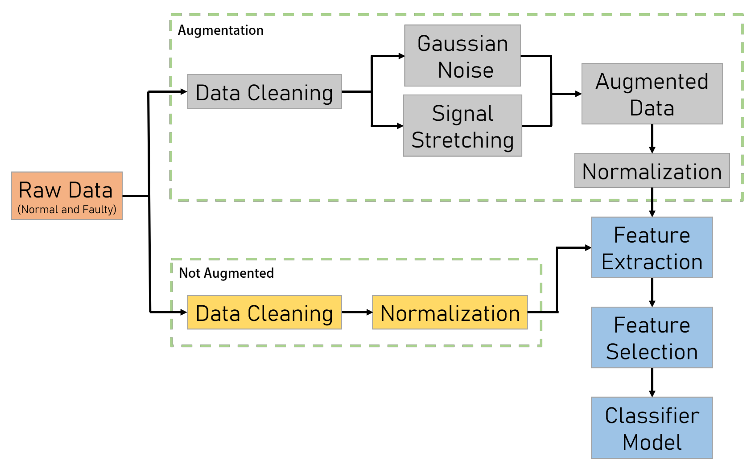
The data collected from the centrifugal pump over one day consisted of 1,048,576 normal data points, 97,912 wear data points, and 109,328 crack data points. The overall framework is illustrated in Figure 2. Before feeding the data into the model, several pre-processing techniques were applied: i) Data cleaning to remove rows with missing values, ii) Normalization to scale the values uniformly without altering their relative differences, iii) Feature extraction to identify relevant features for model training, and iv) Feature selection to choose the most significant features using a threshold of 0.9. For the augmented data, we performed data augmentation on the faulty data using a combination of Gaussian noise and signal stretching. Gaussian noise was added to the raw data with a standard deviation of 0.15, and signal stretching was applied with a stretch factor of 0.2. The augmented data was then combined with the original faulty data, increasing the data size to three times the original size before normalization. After feature selection, the normal data was reduced to 5,825 features, while the augmented faulty data, comprising wear and crack data, was reduced to 1,619 and 1,822 features, respectively. Without data augmentation, the selected features for the faulty data were reduced to 539 and 607, respectively. For training the classifier models—support vector classifier (SVC), random forest (RF), and gradient boosting (GB)—we used 70% of the data for training and 30% for testing. The parameters of the classifier models are shown in Table 1. The performance of each model, both before and after augmentation, was evaluated in terms of accuracy, precision, recall, F1-score, confusion matrix, and 5-fold cross-validation.

3.2. LSTM-AE-GAN for Anomaly Detection

The LSTM-Autoencoder-GAN (LSTMAEGAN) model is integrated to effectively handle and generate sequential data. This hybrid model leverages the strengths of LSTM networks for sequence reconstruction and GANs for generating realistic synthetic sequences. The LSTM-AE serves as the foundation of the model. It consists of an encoder that processes input sequences through an LSTM layer with 128 units, compressing them into a latent representation. This latent space representation is then expanded to reconstruct the original sequence length using a decoder LSTM layer with 128 units. The final output is produced through a TimeDistributed Dense layer that matches the original sequence dimensions. This architecture is detailed in Table 2. Following the autoencoder, the GAN framework introduces two additional components: the generator and the discriminator. The generator network creates synthetic sequences from random noise. It begins with a Dense layer with 100 units, followed by a LeakyReLU activation and BatchNormalization to stabilize training. The generator then uses another Dense layer with a tanh activation function to output sequences reshaped to the desired dimensions, as shown in Table 3. The discriminator is tasked with distinguishing between real and fake sequences. It comprises two LSTM layers: the first with 128 units and the second with 64 units, designed to process the sequences and extract features. The final layer is a Dense layer with a sigmoid activation function that outputs the probability of the sequence being real or fake. This setup is detailed in Table 4. Training the model involves a two-phase process. First, the discriminator is trained to differentiate actual sequences from those generated by the generator. Then, the generator is trained to improve its ability to produce sequences that can effectively fool the discriminator. This iterative training process enhances the model’s capability to generate high-quality synthetic sequences and refine sequence reconstruction. Overall, the LSTMAEGAN model leverages advanced sequence processing and generative techniques to handle time series data, making it a robust tool for anomaly detection and synthetic data generation tasks. Combining the autoencoder’s reconstruction capabilities with the GAN’s generative power, the model offers a comprehensive approach to managing and analyzing sequential data.

3.3. Performance Metrics

The performance of machine learning models is commonly assessed using key metrics: accuracy, precision, recall, and F1 score. These metrics are particularly important in evaluating models on imbalanced datasets. In this analysis, the Support Vector Classifier (SVC), Random Forest (RF), and Gradient Boost (GD) models were evaluated using 5-fold cross-validation to ensure the robustness of the results. Additionally, the LSTMAEGAN model was assessed using precision, recall, F1 score, and a reconstruction error threshold, reflecting its role as a generative model. The SVC aims to find the optimal hyperplane that maximizes the margin between classes, generally performing well in accuracy. However, accuracy alone can be misleading in imbalanced datasets, making precision and recall critical for a more comprehensive evaluation. The SVC typically exhibits strong precision but may vary in recall, impacting the F1 score. On one hand, The RF model, an ensemble method of decision trees, performs exceptionally well in accuracy due to its ability to capture complex patterns. It tends to achieve high precision and recall, resulting in a balanced F1 score. On the other hand, the GD model, which incrementally builds an ensemble, also shows high accuracy and precision but may sacrifice recall, leading to a moderate F1 score depending on the model’s focus on correcting specific errors. However, the LSTMAEGAN model, combining LSTM Autoencoder with a Generative Adversarial Network (GAN), is evaluated on its ability to correctly reconstruct regular sequences (precision) and detect true anomalies (recall). The F1 score, balancing precision and recall, along with the reconstruction error threshold, determines the model’s effectiveness in anomaly detection. Each model’s performance metrics highlight its strengths and weaknesses: SVC excels in precision, RF and GD offer balanced performance, and LSTMAEGAN specializes in anomaly detection with its unique reconstruction error threshold. This comprehensive evaluation provides a robust understanding of the models’ abilities in classification and anomaly detection.

The mathematical expressions are as follows:

A c c u r a c y = \frac{T P + T N}{T P + T N + F P + F N}

(18)

P r e c i s i o n = \frac{T P}{T P + F P}

(19)

R e c a l l = \frac{T P}{T P + F N}

(20)

F 1 S c o r e = 2 \times \frac{P r e c i s i o n \times R e c a l l}{P r e c i s i o n ∔ R e c a l l}

(21)

R e c o n s t r u c t i o n E r r o r = ∥x - \hat{x}∥

(22)

where TP is the number of true positives, TN is the number of true negatives, FP is the number of false positives, FN is the number of false negatives, x is the original input sequence,

\hat{x}

is the reconstructed sequence by the model,

∥\cdot∥

and represents a norm, typically the Euclidean norm.

4. Experimental Study

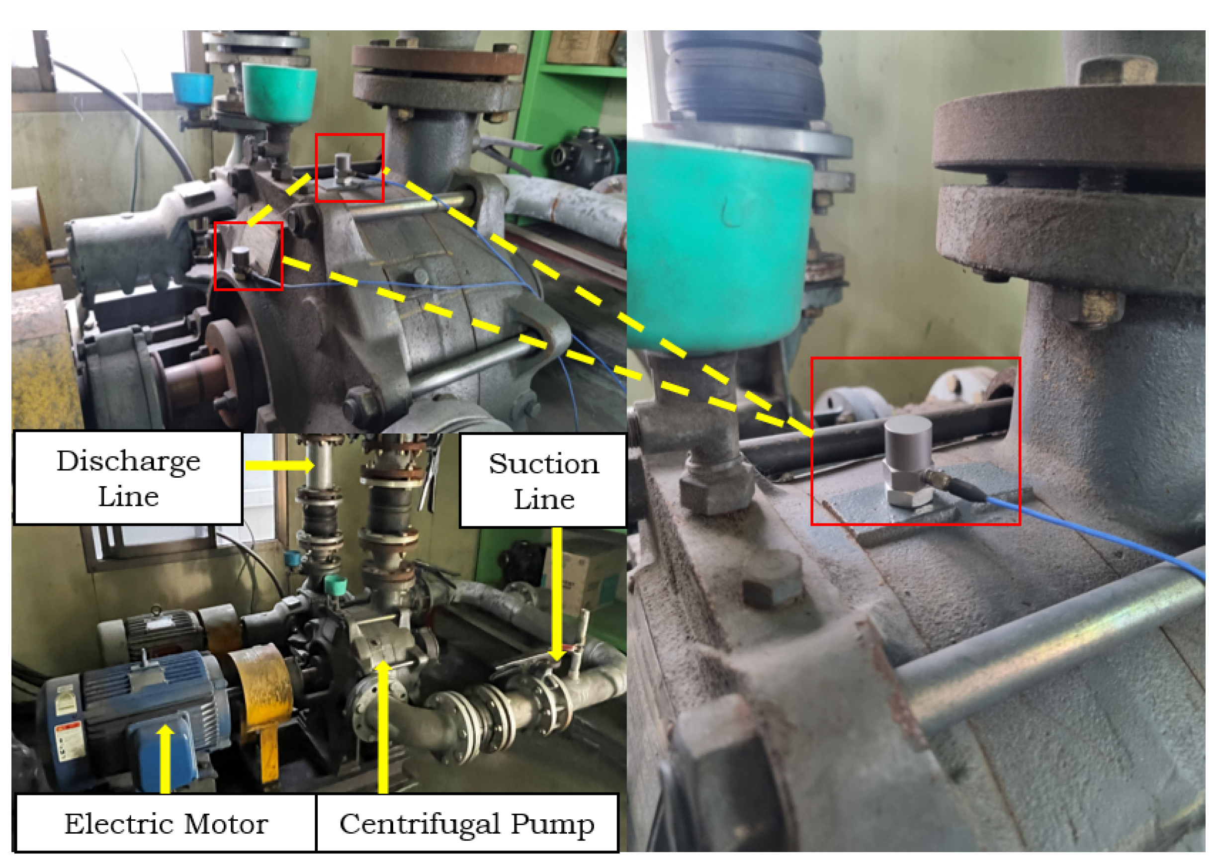
Figure 3 shows the vibration sensor placement for validation of the proposed method in this study. Our experimental study of a centrifugal water pump focused on analyzing vibrations to detect potential anomalies and improve maintenance strategies. Two vibration sensors were strategically attached to the centrifugal pump to capture data from different points, ensuring a comprehensive understanding of the pump’s operational state.

4.1. Data Collection and Preprocessing

The sensors meticulously recorded vibration signals continuously, generating raw data that underwent several meticulous preprocessing steps. Initially, the data was cleaned with precision to remove any noise or irrelevant information. The signals were then normalized using Min-Max scaling to ensure a consistent range and facilitate comparison across different datasets. Sequences were created from the time-series data with careful consideration to refine the data further, allowing for more structured input suitable for machine learning models.

4.2. Data Augmentation and Implementation

Traditional data augmentation techniques, such as adding Gaussian noise and signal stretching, are straightforward yet effective in increasing dataset diversity. Gaussian noise enhances model robustness by introducing random variations, while signal stretching adjusts signal timing without altering content, allowing the model to learn from different signal durations. In contrast, advanced data augmentation using LSTMAEGAN leverages deep learning to generate synthetic data that closely mimics the original dataset’s complex patterns. This method preserves temporal dependencies and produces more diverse and high-quality augmentations, significantly improving model generalization and performance, especially in detecting anomalies or rare events. In our implementation, these augmented datasets were used to train anomaly detection algorithms, enhancing the models’ accuracy and robustness. By combining traditional and advanced augmentation techniques, we significantly improved the system’s ability to detect and classify anomalies in vibration data, leading to more effective maintenance strategies for centrifugal pumps. This study underscores the crucial role of data augmentation in predictive maintenance and highlights the potential of advanced machine learning techniques in improving the reliability and efficiency of industrial equipment.

5. Results and Discussion

5.1. Time-frequency Signal Processing

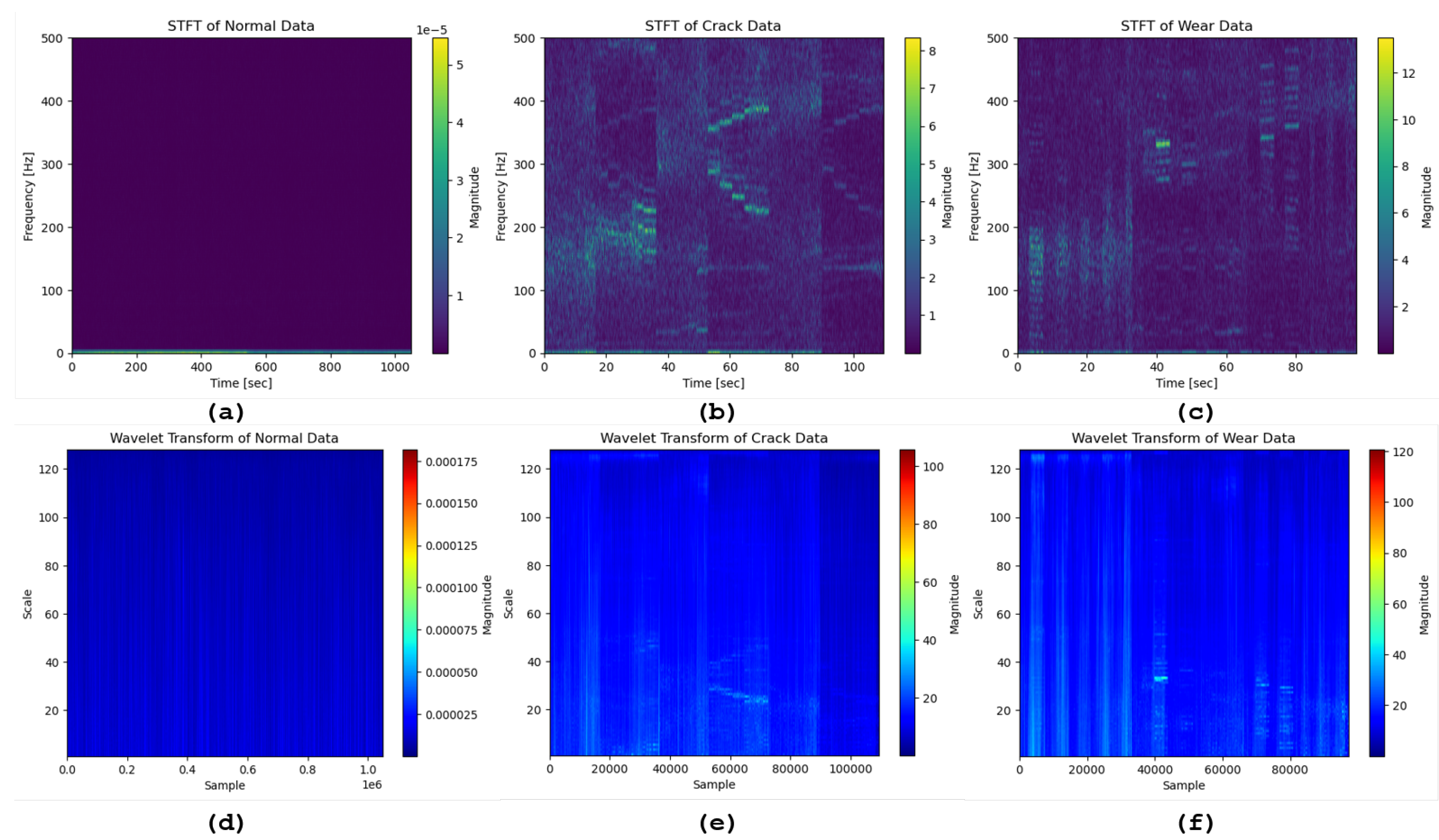
Figure 4 illustrates the application of time-frequency analysis techniques—Short-time Fourier transform (STFT) and continuous wavelet transform (CWT)—to vibration signals from normal, crack, and wear conditions. STFT (top row) provides a view of how the signal’s frequency content changes over time. The STFT captures the frequency content over time, while the CWT provides a time-frequency representation that highlights varying scales of the signals. This technique is advantageous for its simplicity and efficiency in identifying consistent frequency components, making it useful for detecting periodic signals. However, its fixed window size limits its ability to simultaneously resolve time and frequency details, potentially missing transient anomalies. CWT (bottom row) offers a more flexible approach by analyzing the signal at multiple scales, thus capturing varying frequency components with better temporal resolution. This adaptability is beneficial for detecting transient or non-stationary features, though it may result in higher computational costs and complexity. When interpreting these plots, it’s crucial to look for distinct changes in frequency patterns and scales, which can indicate the presence of anomalies or faults in the signal. Figure 5 showcases the Hilbert transform’s ability to extract amplitude envelope and instantaneous frequency information from vibration signals under normal, crack, and wear conditions. The HT is valuable for analyzing non-stationary signals, providing insights into the amplitude modulation and instantaneous frequency crucial for fault detection and condition monitoring. Its primary advantage lies in its capability to reveal phase information and the time-varying frequency of signals. However, the HT may be sensitive to noise and less effective for signals with overlapping frequency components. In these plots, observe the amplitude envelope for changes in signal strength and the instantaneous frequency plot for variations in frequency, which can highlight anomalies or deviations from normal operating conditions. This analysis helps understand the signal’s dynamic behavior and identify potential faults.

5.2. Statistical Feature Engineering

Statistical feature engineering is a critical step in the preprocessing phase of machine learning, especially in tasks involving time-series or sequential data, such as vibration analysis in predictive maintenance. By transforming raw data into meaningful statistical features, we can capture essential characteristics that help in distinguishing between normal and abnormal behavior in systems like centrifugal pumps. Table 5 shows the time domain statistical features extracted from the vibration dataset.

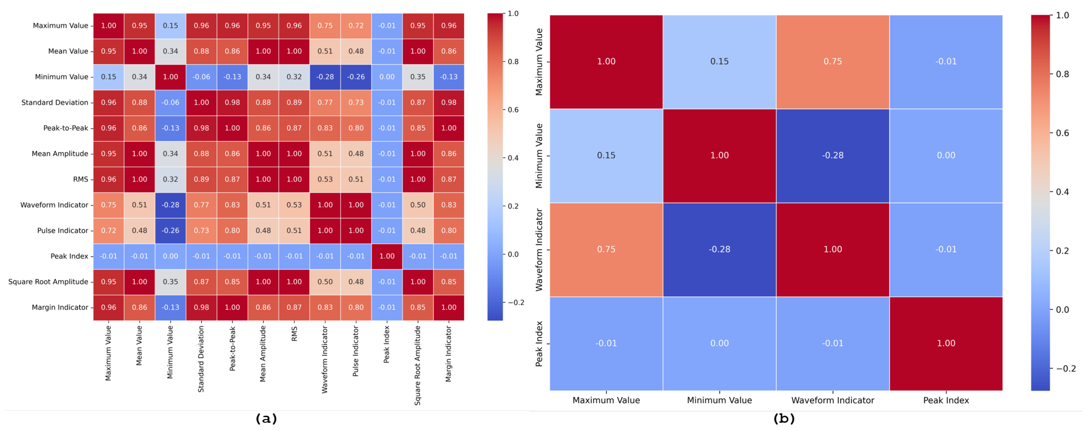
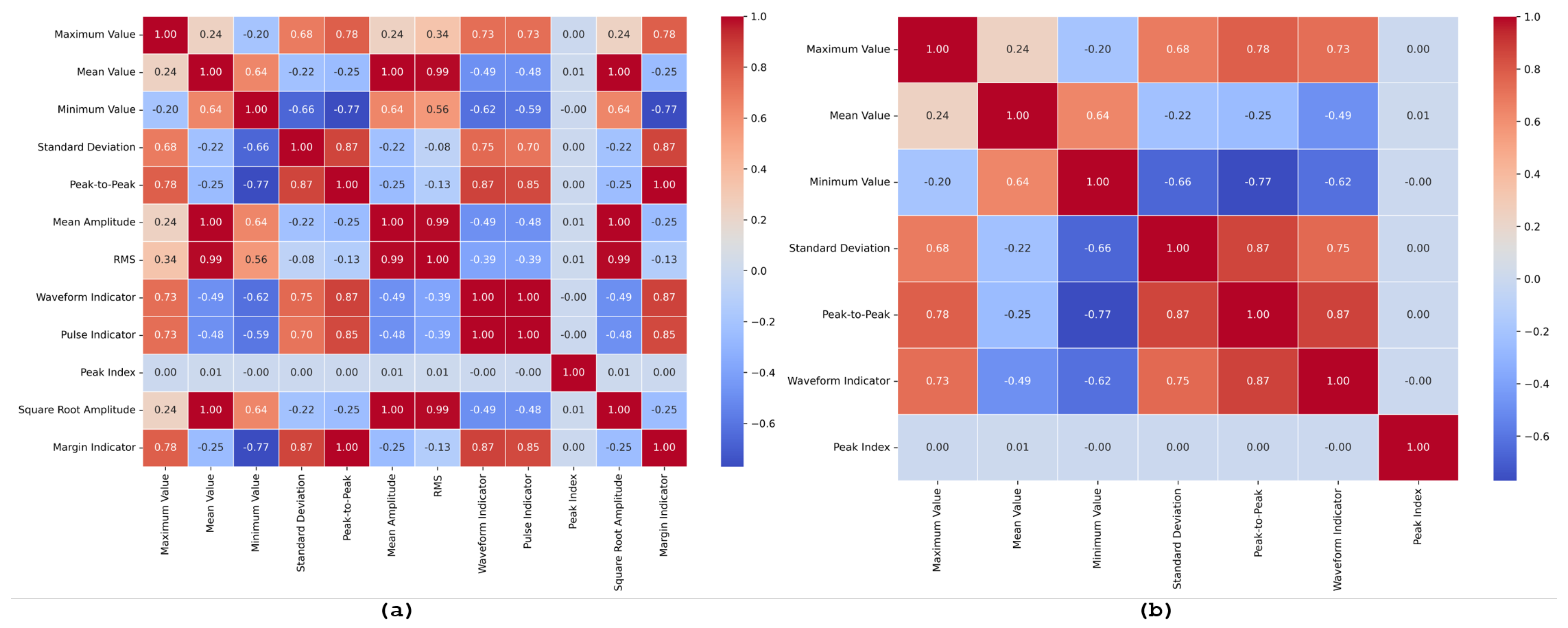
Before data augmentation, the correlation plot of the extracted statistical features in Figure 6(a) provides insights into the relationships among the twelve features: maximum value, mean value, minimum value, standard deviation, peak-to-peak, mean amplitude, RMS, waveform factor, pulse indicator, peak index, square root amplitude, and margin indicator. This analysis helps in understanding how these features are interrelated and highlights potential multicollinearity issues. High correlations, particularly those above 0.9, indicate that several features might convey similar information, which can lead to redundancy and decreased model efficiency. Applying a Pearson correlation threshold of 0.9 before augmentation led to the selection of a more streamlined feature set: maximum value, minimum value, waveform indicator, and peak index, as shown in Figure 6(b). These features were chosen for their lower inter-correlation, ensuring that each provides distinct and valuable information for the model. This selection process helps in reducing the complexity of the model, making it more interpretable and potentially more accurate. DA, through techniques like Gaussian noise addition and signal stretching, plays a significant role in enhancing the dataset. Augmentation increases the diversity of the data, helping to mitigate overfitting by providing the model with more varied examples. After augmentation, the feature set expands to include additional features such as standard deviation and peak-to-peak, which were previously excluded. This change indicates that augmentation can reveal additional meaningful relationships in the data, contributing to a more robust and generalizable model. The significance of data augmentation is thus evident in its ability to enrich the dataset, enabling the selection of a broader and more informative set of features for model training.

The correlation plot of the extracted statistical features in Figure 7(a) reveals the relationships among the twelve features: maximum value, mean value, minimum value, standard deviation, peak-to-peak, mean amplitude, RMS, waveform factor, pulse indicator, peak index, square root amplitude, and margin indicator. This plot is essential for identifying multicollinearity, where features are highly correlated, potentially leading to redundancy and reduced model performance. High correlations, particularly those above 0.9, indicate that some features provide overlapping information, which can affect the robustness and generalization of the model.

To address this, a Pearson correlation threshold of 0.9 was applied, as shown in Figure 7(b). After applying this threshold, the selected features—maximum value, mean value, minimum value, standard deviation, peak-to-peak, waveform indicator, and peak factor—were retained. These features demonstrate lower inter-correlation, ensuring that the selected features are more independent and contribute uniquely to the model. This selection process not only simplifies the feature set but also enhances the model’s ability to distinguish between different conditions without being influenced by redundant information. The reduced feature set contributes to a more efficient and interpretable model, improving its predictive performance and reliability.

5.3. Gaussian Noise and Signal Stretching

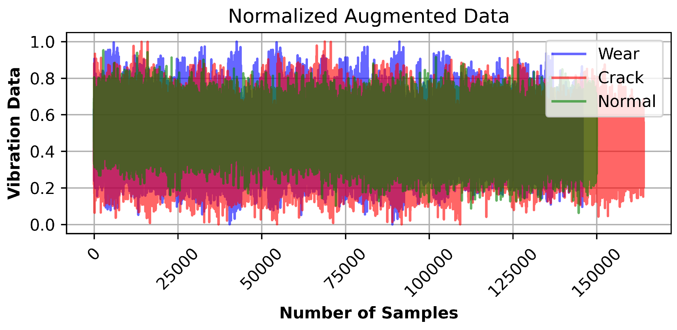
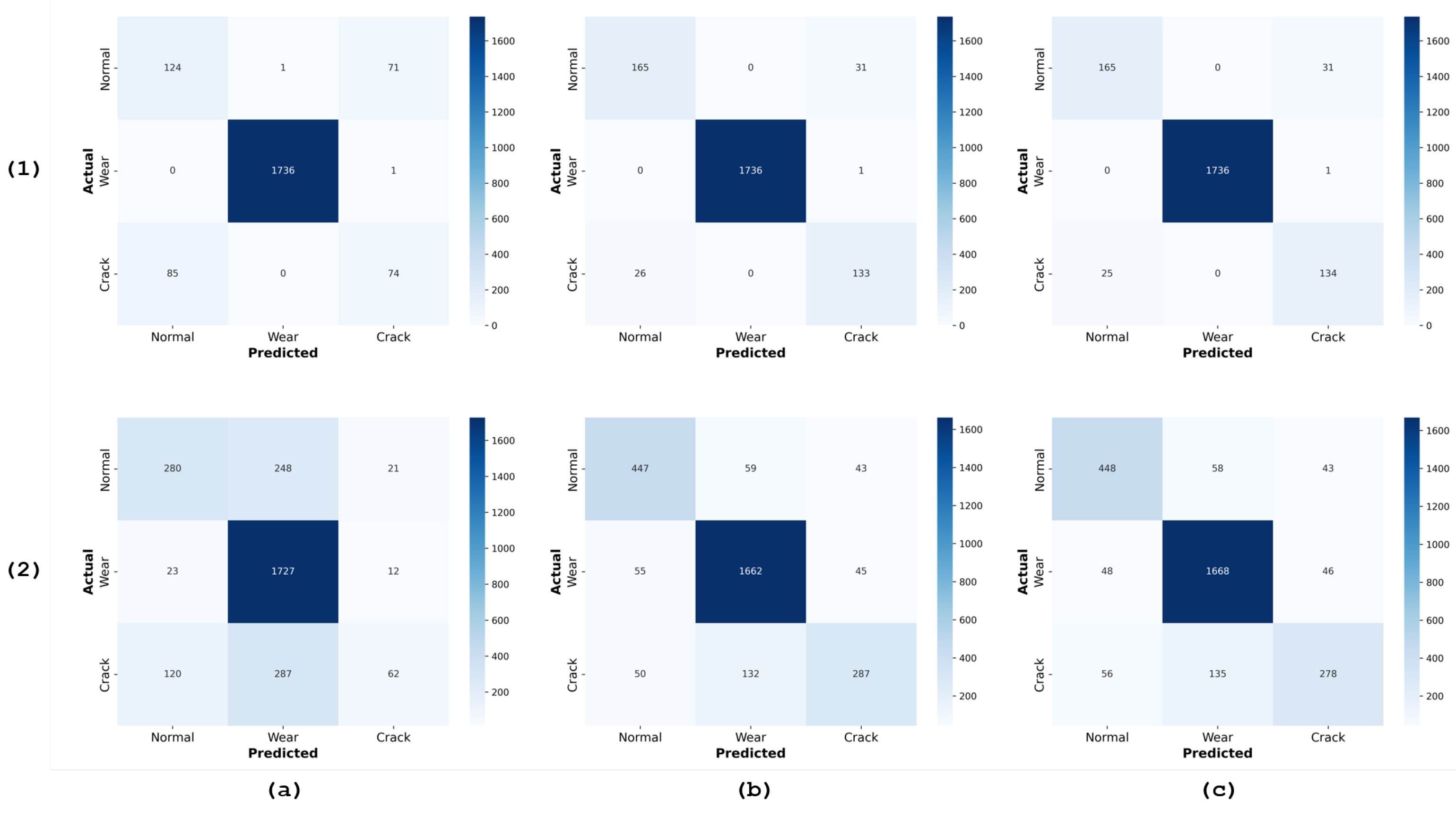
Gaussian noise (GN) and signal stretching (SS) are data augmentation techniques aimed at improving the robustness and generalization of machine learning models by increasing the diversity of the training dataset. The process involved applying these augmentations to the raw data, calculating the weighted average, and extracting statistical features. Figure 8 shows the normalized augmented dataset for the three class labels. These features were then selected based on a set threshold before being fed into three machine learning classifiers: Support Vector Classifier (SVC), Random Forest (RF), and Gradient Boosting (GB). These classifiers were chosen for their different approaches to handling data and their potential to demonstrate the impact of data augmentation on model performance. Below, we discuss the results before and after augmentation, focusing on the impact on the actual label predictions across the three models. Figure 9 shows the confusion matrix plot for the classifier model before and after augmentation.

Before data augmentation, the classifiers demonstrated a commendable performance, as reflected in their high accuracy, precision, recall, and F1 scores. For instance, the SVC model showed strong performance, particularly in precision and recall for the majority class (wear), although it faced challenges with minority classes such as regular and crack. SVC results before augmentation:

Normal: Out of 196 samples, 124 were correctly predicted as usual, 71 were misclassified as crack, and only one misclassified as wear.
Wear: Among 1737 samples, the model performed exceptionally well, correctly predicting 1736 as wear, with just one misclassified as crack.
Crack: Out of 159 crack samples, 74 were correctly identified as crack, but a significant number (85) were misclassified as normal.

These results underscore the critical issue of class imbalance, where the model is biased towards the majority class (wear), resulting in a higher number of misclassifications for the minority classes (normal and crack). Addressing this imbalance is crucial for a more balanced and accurate model performance.

After applying GN and SS, the number of data samples increased significantly, introducing more variability into the training set and helping mitigate some of the class imbalance. This increase in data variability, while leading to a decrease in performance metrics such as accuracy, precision, recall, and F1 score, also led to an increase in true label predictions for the augmented data, particularly for the normal and crack classes. This indicates a promising improvement in the model’s ability to recognize these previously underrepresented classes. SVC results after augmentation:

Normal: The normal class saw a substantial increase in sample size to 549, with 280 correctly predicted as normal, though 248 were misclassified as wear and 21 as crack.
Wear: Out of 1762 wear samples, 1727 were correctly identified, with a slight increase in misclassifications into the normal (23) and crack (12) classes.
Crack: The crack class also benefited from augmentation, increasing to 469 samples. Here, 120 were misclassified as normal, 287 as wear, and 62 correctly identified as crack.

These results indicate that while augmentation led to a slight decrease in overall performance metrics, the increase in true label predictions for normal and crack classes is significant. The improvement in the model’s ability to detect these classes suggests that data augmentation helped address the data imbalance issue, providing a more diverse training set that allowed the classifiers to generalize better to previously underrepresented classes. The augmentation process demonstrates that while traditional metrics like accuracy, precision, and recall might decrease, the true positive rate for minority classes can improve, leading to a more balanced model performance across different classes. This is particularly evident in the confusion matrix results, where the post-augmentation predictions for normal and crack samples increased significantly across all three models. This improvement can be attributed to the augmentation techniques creating more diverse and representative samples, which reduce the model’s bias towards the majority class.

Random forest (RF) results before augmentation:

Normal: Out of 196 normal samples, 165 were correctly classified, but 31 were misclassified as crack.
Wear: The RF model performed excellently in the wear class, correctly classifying 1,736 out of 1,737 samples and misclassifying only one as a crack.
Crack: For crack samples, 133 out of 159 were correctly identified, but 26 were incorrectly labeled as normal.

After Augmentation:

Normal: Post-augmentation, the number of normal samples increased to 549, with 447 correctly predicted. This represents a significant improvement in the true positive rate for normal samples, a key benefit of data augmentation. However, the model now misclassified 59 samples as wear and 43 as crack, introducing more variability in misclassification.
Wear: Among the 1,762 wear samples, 1,662 were correctly identified, showing a slight decline from the pre-augmentation performance. 55 were misclassified as normal, and 45 were classified as cracks.
Crack: For crack samples, the model correctly classified 287 out of 469 samples. However, the increase in misclassifications, particularly into the wear category (132 samples), indicates that while the model’s ability to detect cracks improved, it also became more prone to confusion between similar classes.

The RF model’s performance metrics slightly declined after augmentation, with a noticeable misclassification increase across all classes. However, the model showed a marked improvement in identifying normal samples, which were previously underrepresented. The increase in true positives for the normal class suggests that the augmented data provided more diverse examples for the model to learn from, reducing bias towards the majority class (wear). The trade-off here is an increase in the number of misclassified samples, particularly for the crack class. This may indicate that the augmented data introduced new complexities that the RF model struggled to generalize.

Gradient boosting (GB) results before augmentation:

Normal: Out of 196 normal samples, 165 were correctly classified, with 31 misclassified as crack, similar to RF.
Wear: The GB model performed almost flawlessly for the wear class, correctly classifying 1,736 out of 1,737 samples, with only one misclassification as crack.
Crack: Among the crack samples, 134 out of 159 were correctly classified, with 25 misclassified as normal.

After Augmentation:

Normal: The sample size for normal increased significantly, with 448 out of 549 samples correctly identified. The misclassification rates were 58 as wear and 43 as crack, showing an improvement in identifying normal samples but with similar misclassification patterns as RF.
Wear: The GB model correctly identified 1,668 out of 1,762 wear samples, showing a slight decline in accuracy compared to the pre-augmentation results. This decline underscores the trade-offs involved in improving class representation through data augmentation.
Crack: The model correctly classified 278 out of 469 crack samples. However, misclassifications increased, with 56 labeled as normal and 135 as wear, indicating a similar challenge in distinguishing cracks from other classes.

The GB model, like RF, decreased overall performance metrics after augmentation, but with an improved true positive rate for the normal class. The augmentation led to a better balance in class representation, particularly for normal and crack samples, which were previously underrepresented. However, the model’s ability to accurately distinguish between similar fault types, especially wear and crack, was somewhat compromised. This suggests that while the augmented data helped address the class imbalance, it also introduced additional complexity that the model had difficulty managing, leading to increased misclassifications.

Table 6 shows the performance metrics involving the accuracy, precision, recall, and f1 score. Data augmentation through Gaussian noise and signal stretching significantly impacted the performance of both the RF and GB models. While traditional performance metrics such as accuracy, precision, and recall decreased, the true positive rates for minority classes (normal and crack) improved. This indicates that the models became better at detecting these underrepresented classes, albeit at the cost of increased misclassification in the more complex fault types (wear and crack). The augmentation process addressed the class imbalance, providing the models with a more diverse set of training examples. However, the introduction of more complex variations in the data likely contributed to the increase in misclassifications. This underscores the need to carefully balance augmentation techniques to ensure that while class representation is improved, the data remains distinguishable by the models.

5.4. LSTM-AE-GAN

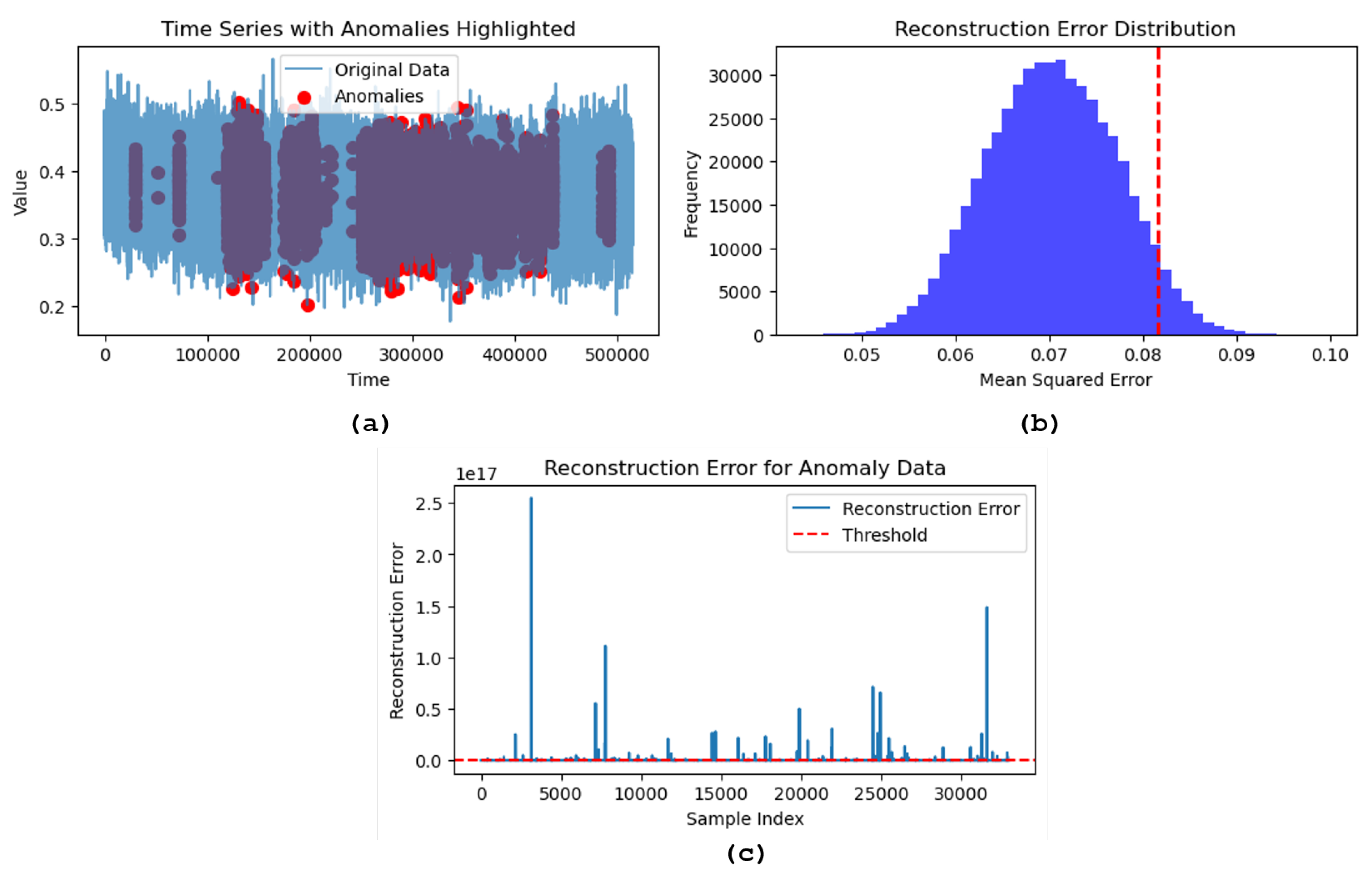
In this study, we employed a comprehensive data preprocessing and augmentation pipeline to enhance the robustness of our diagnostic models. We collected vibration data from centrifugal pumps, which was first scaled using the MinMaxScaler to normalize the values. The data was then segmented into sequences of 100 time steps each, ensuring that temporal patterns in the vibration data were preserved. This sequential data was divided into training and testing sets, with 20% reserved for testing. We implemented an LSTM-based autoencoder to capture the normal behavior of the pump. The autoencoder was trained on the training sequences, and its performance was evaluated on the test sequences. The reconstruction error, measured as Mean Squared Error (MSE), was used as an indicator of anomalies. The reconstruction error distribution was analyzed, and a threshold of 2.115 was set at the 95th percentile for anomaly detection. Anomalies were identified as those sequences with reconstruction errors exceeding this threshold. To further augment our dataset and improve anomaly detection, we developed a Generative Adversarial Network (GAN) consisting of a generator and discriminator. The GAN was trained to generate synthetic sequences that resemble the real vibration data, which were used to enhance the training set. This approach aimed to introduce additional variability and improve the model’s generalization capabilities. The performance of the anomaly detection model was evaluated using key metrics, including accuracy, precision, recall, and F1 score. The results are as follows: Accuracy: 1.0, Precision: 1.0, Recall: 0.98, and F1 Score: 0.99. The confusion matrix further supported these findings, with the model correctly identifying 2058016 normal sequences and 205802 anomalies, while misclassifying only a small number of sequences. The reconstruction error distribution was visualized to understand the model’s error characteristics better. A histogram of the MSE values revealed that most errors were low, with a distinct separation for sequences classified as anomalies. Additionally, a time series plot of the vibration data highlighted the detected anomalies as shown in Figure 10, providing clear visual confirmation of the model’s effectiveness. The results demonstrate that the combination of LSTM autoencoder and GAN-based data augmentation significantly improves the accuracy and reliability of anomaly detection in centrifugal pumps. The model’s ability to detect subtle deviations in the vibration patterns ensures early identification of potential faults, making it a valuable tool for predictive maintenance in industrial settings.

6. Conclusions

In this study, we conducted an extensive experiment on a centrifugal water pump using vibration sensors to monitor and analyze the system’s operational state. Two strategically positioned sensors captured detailed vibration data, which formed the foundation of our analysis.

Initially, we employed traditional data augmentation techniques, incorporating Gaussian noise and signal processing methods to enhance the dataset. Statistical features based on time were then extracted, and a weighted average of the augmented data was calculated to ensure a robust representation of the vibration patterns. This processed data was subsequently input into three different classifier models—Support Vector Classifier (SVC), Random Forest (RF), and Gradient Descent (GD). By implementing a 5-fold cross-validation, we ensured the reliability of our results, calculating the average across key performance metrics: accuracy, precision, recall, and F1 score.

Recognizing the limitations of traditional augmentation methods, we advanced our approach by integrating Long Short-Term Memory (LSTM), Autoencoder (AE), and Generative Adversarial Network (GAN) models for more sophisticated data augmentation. This advanced LSTM-AE-GAN model was also utilized to perform anomaly detection, distinguishing between normal and anomalous operation states of the pump.

The comparative analysis between traditional and advanced methods revealed that the LSTM-AE-GAN approach significantly improved the model’s ability to detect anomalies, demonstrating the potential of deep learning techniques in enhancing the accuracy and reliability of predictive maintenance systems. Our results underscore the importance of adopting advanced data augmentation and deep learning models for more effective and precise anomaly detection in industrial applications. This study not only showcases the efficacy of modern techniques but also sets the stage for future research in optimizing predictive maintenance strategies.

Author Contributions

Conceptualization D.K., A.B.K., and D.D.; methodology D.K., A.B.K., and D.D.,software D.K., A.B.K., and D.D., and J.-W.H.; validation D.K., A.B.K., and D.D.; formal analysis D.K., A.B.K., and D.D.; investigation D.K., A.B.K., and D.D.; data curation D.K., A.B.K., and D.D., writing—original draft preparation A.B.K.; and D.D.; writing—review and editing A.B.K.; and D.D.; and visualization D.K., A.B.K., and D.D., resources and supervision J.-W.H.; project administration J.-W.H.; and funding acquisition J.-W.H. All authors have read and agreed to the published version of the manuscript.

Funding

This work was supported by the Innovative Human Resource Development for Local Intellectualization program through the Institute of Information & Communications Technology Planning & Evaluation(IITP) grant funded by the Korean government(MSIT) (IITP-2024-2020-0-01612).

Institutional Review Board Statement

Not applicable.

Informed Consent Statement

Not applicable.

Data Availability Statement

The data presented in this study are available on request from the corresponding author. The data are not publicly available due to laboratory regulations.

Conflicts of Interest

The authors declare no conflicts of interest.

References

Espina-Romero, L.; Guerrero-Alcedo, J.; Goñi Avila, N.; Noroño Sánchez, J.G.; Gutiérrez Hurtado, H.; Quiñones Li, A. Industry 5.0: Tracking Scientific Activity on the Most Influential Industries, Associated Topics, and Future Research Agenda. Sustainability 2023, 15, 5554. [Google Scholar] [CrossRef]
Mladineo, M.; Celent, L.; Milković, V.; Veža, I. Current State Analysis of Croatian Manufacturing Industry with Regard to Industry 4.0/5.0. Machines 2024, 12, 87. [Google Scholar] [CrossRef]
Jamwal, A.; Agrawal, R.; Sharma, M.; Giallanza, A. Industry 4.0 Technologies for Manufacturing Sustainability: A Systematic Review and Future Research Directions. Appl. Sci 2021, 11, 5725. [Google Scholar] [CrossRef]
Konstantinidis, F.K.; Myrillas, N.; Mouroutsos, S.G.; Koulouriotis, D.; Gasteratos, A. Assessment of Industry 4.0 for Modern Manufacturing Ecosystem: A Systematic Survey of Surveys. Machines 2022, 10, 746. [Google Scholar] [CrossRef]
Webert, H.; Döß, T.; Kaupp, L.; Simons, S. Fault Handling in Industry 4.0: Definition, Process and Applications. Sensors 2022, 22, 2205 [CrossRef]. [Google Scholar] [CrossRef]
Angelopoulos, A.; Michailidis, E.T.; Nomikos, N.; Trakadas, P.; Hatziefremidis, A.; Voliotis, S.; Zahariadis, T. Tackling Faults in the Industry 4.0 Era—A Survey of Machine-Learning Solutions and Key Aspects. Sensors 2020, 20, 109. [Google Scholar] [CrossRef]
Hadi, R.H.; Hady, H.N.; Hasan, A.M.; Al-Jodah, A.; Humaidi, A.J. Improved Fault Classification for Predictive Maintenance in Industrial IoT Based on AutoML: A Case Study of Ball-Bearing Faults. Processes 2023, 11, 1507. [Google Scholar] [CrossRef]
Kim, S.W.; Kong, J.H.; Lee, S.W.; et al. Recent Advances of Artificial Intelligence in Manufacturing Industrial Sectors: A Review. Int. J. Precis. Eng. Manuf. 2022, 23, 111–129. [Google Scholar] [CrossRef]
Aldoseri, A.; Al-Khalifa, K.N.; Hamouda, A.M. Re-Thinking Data Strategy and Integration for Artificial Intelligence: Concepts, Opportunities, and Challenges. Appl. Sci. 2023, 13, 7082. [Google Scholar] [CrossRef]
Cao, K.; Zhang, T.; Huang, J. Advanced Hybrid LSTM-Transformer Architecture for Real-Time Multi-Task Prediction in Engineering Systems. Sci. Rep. 2024, 14, 4890. [Google Scholar] [CrossRef]
Törngren, M.; Grogan, P.T. How to Deal with the Complexity of Future Cyber-Physical Systems? Designs 2018, 2, 40. [Google Scholar] [CrossRef]
Yan, W.; Wang, J.; Lu, S.; Zhou, M.; Peng, X. A Review of Real-Time Fault Diagnosis Methods for Industrial Smart Manufacturing. Processes 2023, 11, 369. [Google Scholar] [CrossRef]
Gültekin, Ö.; Cinar, E.; Özkan, K.; Yazıcı, A. Real-Time Fault Detection and Condition Monitoring for Industrial Autonomous Transfer Vehicles Utilizing Edge Artificial Intelligence. Sensors 2022, 22, 3208. [Google Scholar] [CrossRef] [PubMed]
Moshrefi, A.; Nabki, F. Advanced Industrial Fault Detection: A Comparative Analysis of Ultrasonic Signal Processing and Ensemble Machine Learning Techniques. Appl. Sci. 2024, 14, 6397. [Google Scholar] [CrossRef]
Mercorelli, P. Recent Advances in Intelligent Algorithms for Fault Detection and Diagnosis. Sensors 2024, 24, 2656. [Google Scholar] [CrossRef]
Mey, O.; Neufeld, D. Explainable AI Algorithms for Vibration Data-Based Fault Detection: Use Case-Adapted Methods and Critical Evaluation. Sensors 2022, 22, 9037. [Google Scholar] [CrossRef]
Łuczak, D. Data-Driven Machine Fault Diagnosis of Multisensor Vibration Data Using Synchrosqueezed Transform and Time-Frequency Image Recognition with Convolutional Neural Network. Electronics 2024, 13, 2411. [Google Scholar] [CrossRef]
Senjoba, L.; Ikeda, H.; Toriya, H.; Adachi, T.; Kawamura, Y. Enhancing Interpretability in Drill Bit Wear Analysis through Explainable Artificial Intelligence: A Grad-CAM Approach. Appl. Sci. 2024, 14, 3621. [Google Scholar] [CrossRef]
Cai, Z.; Ma, W.; Wang, X.; Wang, H.; Feng, Z. The Performance Analysis of Time Series Data Augmentation Technology for Small Sample Communication Device Recognition. IEEE Transactions on Reliability 2023, 72(2), 574–585. [Google Scholar] [CrossRef]
Jiang, X.; Ge, Z. Data Augmentation Classifier for Imbalanced Fault Classification. IEEE Transactions on Automation Science and Engineering 2021, 18(3), 1206–1217. [Google Scholar] [CrossRef]
Shao, S.; Wang, P.; Yan, R. Generative Adversarial Networks for Data Augmentation in Machine Fault Diagnosis. Computers in Industry 2019, 106, 85–93. [Google Scholar] [CrossRef]
Ma, L.; Ding, Y.; Wang, Z.; Wang, C.; Ma, J.; Lu, C. An Interpretable Data Augmentation Scheme for Machine Fault Diagnosis Based on a Sparsity-Constrained Generative Adversarial Network. Expert Systems with Applications 2021, 182, 115234. [Google Scholar] [CrossRef]
Li, X.; Zhang, W.; Ding, Q.; Sun, J.-Q. Intelligent Rotating Machinery Fault Diagnosis Based on Deep Learning Using Data Augmentation. Journal of Intelligent Manufacturing.
Iwana, B.K.; Uchida, S. An Empirical Survey of Data Augmentation for Time Series Classification with Neural Networks. PLoS ONE 2021, 16(7), e0254841. [Google Scholar] [CrossRef] [PubMed]
Wei, J.; Zou, K. EDA: Easy Data Augmentation Techniques for Boosting Performance on Text Classification Tasks. In Proceedings of the 2019 Conference on Empirical Methods in Natural Language Processing and the 9th International Joint Conference on Natural Language Processing (EMNLP-IJCNLP), Hong Kong, China, 2019; Association for Computational Linguistics. pp. 6382–6388. [Google Scholar]
Jeong, H.; Jeung, S.; Lee, H.; Kwon, J. BiVi-GAN: Bivariate Vibration GAN. Sensors 2024, 24, 1765. [Google Scholar] [CrossRef]
Stathatos, E.; Tzimas, E.; Benardos, P.; Vosniakos, G.-C. Convolutional Neural Networks for Raw Signal Classification in CNC Turning Process Monitoring. Sensors 2024, 24, 1390. [Google Scholar] [CrossRef]
Cui, W.; Ding, J.; Meng, G.; Lv, Z.; Feng, Y.; Wang, A.; Wan, X. Fault Diagnosis of Rolling Bearings in Primary Mine Fans under Sample Imbalance Conditions. Entropy 2023, 25, 1233. [Google Scholar] [CrossRef]
Wang, H.; Li, Y.; Jin, Y.; Zhao, S.; Han, C.; Song, L. Remaining Useful Life Prediction Method Enhanced by Data Augmentation and Similarity Fusion. Vibration 2024, 7, 560–581. [Google Scholar] [CrossRef]
Lyu, P.; Zhang, H.; Yu, W.; Liu, C. A Novel Model-Independent Data Augmentation Method for Fault Diagnosis in Smart Manufacturing. Procedia CIRP 2022, 107, 949–954. [Google Scholar] [CrossRef]
Ramteke, D.S.; Parey, A.; Pachori, R.B. A New Automated Classification Framework for Gear Fault Diagnosis Using Fourier–Bessel Domain-Based Empirical Wavelet Transform. Machines 2023, 11, 1055. [Google Scholar] [CrossRef]
Yan, Z.; Liu, H.; Tao, L.; Ma, J.; Cheng, Y. A Universal Feature Extractor Based on Self-Supervised Pre-Training for Fault Diagnosis of Rotating Machinery under Limited Data. Aerospace 2023, 10, 681. [Google Scholar] [CrossRef]
Afridi, Y.S.; Hasan, L.; Ullah, R.; Ahmad, Z.; Kim, J.-M. LSTM-Based Condition Monitoring and Fault Prognostics of Rolling Element Bearings Using Raw Vibrational Data. Machines 2023, 11, 531. [Google Scholar] [CrossRef]
Chen, L.; Li, Z.; Shi, W.; Li, W. Research on Fault Detection and Automatic Diagnosis Technology of Water Hammer in Centrifugal Pump. Appl. Sci. 2024, 14, 5606. [Google Scholar] [CrossRef]
Yang, X.; Xu, X.; Wang, Y.; Liu, S.; Bai, X.; Jing, L.; Ma, J.; Huang, J. The Fault Diagnosis of a Plunger Pump Based on the SMOTE + Tomek Link and Dual-Channel Feature Fusion. Appl. Sci. 2024, 14, 4785. [Google Scholar] [CrossRef]
Viswanathan, C.; Venkatesh, S.N.; Dhanasekaran, S.; Mahanta, T.K.; Sugumaran, V.; Lakshmaiya, N.; Ramasamy, S.N. Deep Learning for Enhanced Fault Diagnosis of Monoblock Centrifugal Pumps: Spectrogram-Based Analysis. Machines 2023, 11, 874. [Google Scholar] [CrossRef]
Alizadeh, J.; Bogdan, M.; Classen, J.; Fricke, C. Support Vector Machine Classifiers Show High Generalizability in Automatic Fall Detection in Older Adults. Sensors 2021, 21, 7166. [Google Scholar] [CrossRef]
Kabir, R.; Watanobe, Y.; Islam, M.R.; Naruse, K.; Rahman, M.M. Unknown Object Detection Using a One-Class Support Vector Machine for a Cloud–Robot System. Sensors 2022, 22, 1352. [Google Scholar] [CrossRef]
Kareem, A.B.; Ejike Akpudo, U.; Hur, J.-W. An Integrated Cost-Aware Dual Monitoring Framework for SMPS Switching Device Diagnosis. Electronics 2021, 10, 2487. [Google Scholar] [CrossRef]
Nadkarni, S.B.; Vijay, G.S.; Kamath, R.C. Comparative Study of Random Forest and Gradient Boosting Algorithms to Predict Airfoil Self-Noise. Eng. Proc. 2023, 59, 24. [Google Scholar] [CrossRef]
Yang, Y.; Li, Y.; Cai, Y.; Tang, H.; Xu, P. Data-Driven Golden Jackal Optimization–Long Short-Term Memory Short-Term Energy-Consumption Prediction and Optimization System. Energies 2024, 17, 3738. [Google Scholar] [CrossRef]
Wang, W.; Ma, B.; Guo, X.; Chen, Y.; Xu, Y. A Hybrid ARIMA-LSTM Model for Short-Term Vehicle Speed Prediction. Energies 2024, 17, 3736. [Google Scholar] [CrossRef]
Moon, Y.; Lee, Y.; Hwang, Y.; Jeong, J. Long Short-Term Memory Autoencoder and Extreme Gradient Boosting-Based Factory Energy Management Framework for Power Consumption Forecasting. Energies 2024, 17, 3666. [Google Scholar] [CrossRef]
Ju, J.; Liu, F.-A. Multivariate Time Series Data Prediction Based on ATT-LSTM Network. Appl. Sci. 2021, 11, 9373. [Google Scholar] [CrossRef]
Yin, Z.; Shao, J.; Hussain, M.J.; Hao, Y.; Chen, Y.; Zhang, X.; Wang, L. DPG-LSTM: An Enhanced LSTM Framework for Sentiment Analysis in Social Media Text Based on Dependency Parsing and GCN. Appl. Sci. 2023, 13, 354. [Google Scholar] [CrossRef]
Kim, T.; Kim, J.; You, I. An Anomaly Detection Method Based on Multiple LSTM-Autoencoder Models for In-Vehicle Network. Electronics 2023, 12, 3543. [Google Scholar] [CrossRef]
Do, J.S.; Kareem, A.B.; Hur, J.-W. LSTM-Autoencoder for Vibration Anomaly Detection in Vertical Carousel Storage and Retrieval System (VCSRS). Sensors 2023, 23, 1009. [Google Scholar] [CrossRef]
Lee, S.; Kareem, A.B.; Hur, J.-W. A Comparative Study of Deep-Learning Autoencoders (DLAEs) for Vibration Anomaly Detection in Manufacturing Equipment. Electronics 2024, 13, 1700. [Google Scholar] [CrossRef]
Lee, J.-H.; Okwuosa, C.N.; Hur, J.-W. Extruder Machine Gear Fault Detection Using Autoencoder LSTM via Sensor Fusion Approach. Inventions 2023, 8, 140. [Google Scholar] [CrossRef]
Lee, J.-G.; Kim, D.-H.; Lee, J.H. Proactive Fault Diagnosis of a Radiator: A Combination of Gaussian Mixture Model and LSTM Autoencoder. Sensors 2023, 23, 8688. [Google Scholar] [CrossRef]
Lachekhab, F.; Benzaoui, M.; Tadjer, S.A.; Bensmaine, A.; Hamma, H. LSTM-Autoencoder Deep Learning Model for Anomaly Detection in Electric Motor. Energies 2024, 17, 2340. [Google Scholar] [CrossRef]
Tang, T.-W.; Kuo, W.-H.; Lan, J.-H.; Ding, C.-F.; Hsu, H.; Young, H.-T. Anomaly Detection Neural Network with Dual Auto-Encoders GAN and Its Industrial Inspection Applications. Sensors 2020, 20, 3336. [Google Scholar] [CrossRef]
Chen, L.; Li, Y.; Deng, X.; Liu, Z.; Lv, M.; Zhang, H. Dual Auto-Encoder GAN-Based Anomaly Detection for Industrial Control System. Appl. Sci. 2022, 12, 4986. [Google Scholar] [CrossRef]
Avola, D.; Cannistraci, I.; Cascio, M.; Cinque, L.; Diko, A.; Fagioli, A.; Foresti, G.L.; Lanzino, R.; Mancini, M.; Mecca, A.; et al. A Novel GAN-Based Anomaly Detection and Localization Method for Aerial Video Surveillance at Low Altitude. Remote Sens. 2022, 14, 4110. [Google Scholar] [CrossRef]
Ewert, P.; Wicher, B.; Pajchrowski, T. Application of the STFT for Detection of the Rotor Unbalance of a Servo-Drive System with an Elastic Interconnection. Electronics 2024, 13, 441. [Google Scholar] [CrossRef]
Yang, X.; Chen, X.; Sun, K.; Xiong, C.; Song, D.; Lu, Y.; Huang, L.; He, S.; Zhang, X. A Wavelet Transform-Based Real-Time Filtering Algorithm for Fusion Magnet Power Signals and Its Implementation. Energies 2023, 16, 4091. [Google Scholar] [CrossRef]
Li, Y.; Lin, J.; Niu, G.; Wu, M.; Wei, X. A Hilbert–Huang Transform-Based Adaptive Fault Detection and Classification Method for Microgrids. Energies 2021, 14, 5040. [Google Scholar] [CrossRef]
Gonçalves, J.P.S.; Fruett, F.; Dalfré Filho, J.G.; Giesbrecht, M. Faults Detection and Classification in a Centrifugal Pump from Vibration Data Using Markov Parameters. Mechanical Systems and Signal Processing 2021, 158, 107694. [Google Scholar] [CrossRef]
Sun, H.; Yuan, S.; Luo, Y. Cyclic Spectral Analysis of Vibration Signals for Centrifugal Pump Fault Characterization. IEEE Sensors Journal 2018, 18(7), 2925–2933. [Google Scholar] [CrossRef]
Sakthivel, N.R.; Nair, B.B.; Elangovan, M.; Sugumaran, V.; Saravanmurugan, S. Comparison of Dimensionality Reduction Techniques for the Fault Diagnosis of Mono Block Centrifugal Pump Using Vibration Signals. Engineering Science and Technology, an International Journal 2014, 17(1), 30–38. [Google Scholar] [CrossRef]
Karagiovanidis, M.; Pantazi, X.E.; Papamichail, D.; Fragos, V. Early Detection of Cavitation in Centrifugal Pumps Using Low-Cost Vibration and Sound Sensors. Agriculture 2023, 13, 1544. [Google Scholar] [CrossRef]
Ahmad, S.; Ahmad, Z.; Kim, J.-M. A Centrifugal Pump Fault Diagnosis Framework Based on Supervised Contrastive Learning. Sensors 2022, 22, 6448. [Google Scholar] [CrossRef]

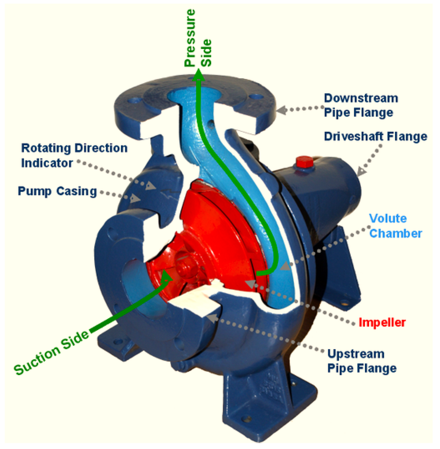
Figure 1. A side cut-through of a centrifugal pump, clearly illustrating key components such as the suction inlet, impeller, pressure outlet, casing, and volute chamber.

Figure 2. Framework for using data augmentation using Gaussian noise and signal stretching

Figure 3. Vibration data collection setup for the water pump system

Figure 4. Time-frequency analysis of vibration signals from different conditions. The top row shows the STFT of vibration data: (a) Normal, (b) Crack, and (c) Wear. The bottom row displays the CWT of the same signals: (d) Normal, (e) Crack, and (f) Wear.

Figure 5. Analysis of vibration signals using the HT. For each dataset (a) Normal, (b) Crack, and (c) Wear, the plot shows the following: (1) The original signal, (2) The amplitude envelope computed from the Hilbert Transform, and (3) The instantaneous frequency derived from the phase of the analytic signal.

Figure 6. Before augmentation (a) Correlation plot of all statistical features, showing the degree of the linear relationship between each pair of features. This plot helps identify multicollinearity among the features. (b) Selected features after applying a Pearson correlation threshold of <0.9, highlighting the features with lower inter-correlation, thus reducing redundancy and improving the robustness of the model.

Figure 7. After augmentation (a) Correlation plot of all statistical features, showing the degree of linear relationship between each pair of features. This plot helps identify multicollinearity among the features. (b) Selected features after applying a Pearson correlation threshold of <0.9, highlighting the features with lower inter-correlation, thus reducing redundancy and improving the robustness of the model.

Figure 8. Plot of the normalized weighted average of Gaussian noise and signal processing under different fault conditions: normal, wear, and crack.

Figure 9. Confusion matrices for the classification performance of three models: (a) SVC, (b) Random Forest, and (c) Gradient Boost. The matrices are presented for each dataset before and after data augmentation. The first set of matrices (1) corresponds to the performance before augmentation, while the second set (2) corresponds to the performance after augmentation. Each matrix shows the classification of vibration signal labels: ’Normal’, ’Crack’, and ’Wear Fault’.

Figure 10. (a) Distribution of reconstruction errors for the dataset, with the red dashed line indicating the chosen threshold for anomaly detection. The histogram shows the frequency of Mean Squared Errors (MSE), helping to visualize the separation between normal and anomalous data points. (b) Time series plot of the original data with anomalies highlighted in red. The anomalies, identified based on the reconstruction error threshold, are marked against the backdrop of the normal data, illustrating the model’s ability to detect deviations over time.

Table 1. Machine learning models and parameter values.

ML Model	Parameter	Value
SVC	gamma, C	scale, 90
RF and GB	n estimators	70

Table 2. Architecture of the LSTM Autoencoder

Layer Type	Units	Activation	Output Shape
Input	-	-	(seq_length, n_features)
LSTM (Encoder)	128	ReLU	(seq_length, 128)
RepeatVector	-	-	(seq_length, 128)
LSTM (Decoder)	128	ReLU	(seq_length, 128)
Dense	n_features	-	(seq_length, n_features)

Table 3. Architecture of the Generator Network

Layer Type	Units	Activation	Output Shape
Dense	100	LeakyReLU	(None, 100)
BatchNormalization	-	-	(None, 100)
Dense	seq_length × n_features	Tanh	(None, seq_length × n_features)
Reshape	-	-	(None, seq_length, n_features)

Table 4. Architecture of the Discriminator Network

Layer Type	Units	Activation	Output Shape
LSTM	128	-	(seq_length, 128)
LSTM	64	-	(64)
Dense	1	Sigmoid	(1)

Table 5. Description of Statistical Features.

Statistical Feature	Description (Mathematical Expression)
Maximum Value	$max (x)$
Mean Value	$μ = \frac{1}{N} \sum_{i = 1}^{N} x_{i}$
Minimum Value	$min (x)$
Standard Deviation	$σ = \sqrt{\frac{1}{N} \sum_{i = 1}^{N} {(x_{i} - μ)}^{2}}$
Peak to Peak	$P 2 P = max (x) - min (x)$
Mean Amplitude	$Mean Amplitude = \frac{1}{N} \sum_{i = 1}^{N} \| x_{i} \|$
RMS	$RMS = \sqrt{\frac{1}{N} \sum_{i = 1}^{N} x_{i}^{2}}$
Waveform Indicator	$Waveform Indicator = \frac{RMS}{Mean Amplitude}$
Pulse Indicator	$Pulse Indicator = \frac{max (x)}{Mean Amplitude}$
Peak Index	$Peak Index = \frac{max (x)}{RMS}$
Square Root Amplitude	$Square Root Amplitude = \sqrt{\frac{1}{N} \sum_{i = 1}^{N} \sqrt{\| x_{i} \|}}$
Margin Indicator	$Margin Indicator = \frac{max (x)}{Square Root Amplitude}$

Table 6. Comparison of performance metrics across different machine learning models (SVC, Random Forest, Gradient Boost) before and after data augmentation, evaluated using 5-fold cross-validation. The table presents the accuracy, precision, recall, and F1-score for each fold, along with the averaged results, highlighting the impact of data augmentation on model performance.

Model	Fold	Before Augmentation				After Augmentation
Model	Fold	Accuracy	Precision	Recall	F1-score	Accuracy	Precision	Recall	F1-score
SVC	1	0.9211	0.9158	0.9211	0.9175	0.7250	0.7123	0.7250	0.6616
	2	0.9273	0.9246	0.9273	0.9231	0.7309	0.7340	0.7309	0.6678
	3	0.9293	0.9282	0.9293	0.9239	0.7147	0.7525	0.7147	0.6379
	4	0.9201	0.9144	0.9201	0.9169	0.7217	0.6930	0.7217	0.6690
	5	0.9159	0.9095	0.9159	0.9109	0.7247	0.6971	0.7247	0.6678
	Averaged	0.9227	0.9185	0.9227	0.9185	0.7234	0.7190	0.7234	0.6608
RF	1	0.9590	0.9602	0.9590	0.9588	0.8621	0.8593	0.8621	0.8594
	2	0.9590	0.9593	0.9590	0.9592	0.8620	0.8606	0.8620	0.8568
	3	0.9631	0.9631	0.9631	0.9631	0.8520	0.8483	0.8520	0.8475
	4	0.9579	0.9550	0.9549	0.9548	0.8589	0.8539	0.8590	0.8526
	5	0.9662	0.9661	0.9662	0.9661	0.8466	0.8423	0.8466	0.8424
	Averaged	0.9604	0.9607	0.9604	0.9604	0.8563	0.8529	0.8563	0.8517
GB	1	0.9600	0.9618	0.9600	0.9598	0.8606	0.8575	0.8606	0.8579
	2	0.9570	0.9576	0.9569	0.9571	0.8558	0.8532	0.8558	0.8489
	3	0.9549	0.9549	0.9549	0.9549	0.8481	0.8430	0.8481	0.8426
	4	0.9631	0.9631	0.9631	0.9631	0.8581	0.8528	0.8581	0.8508
	5	0.9579	0.9579	0.9579	0.9579	0.8427	0.8372	0.8427	0.8369
	Averaged	0.9586	0.9591	0.9586	0.9586	0.8531	0.8487	0.8531	0.8474

Disclaimer/Publisher’s Note: The statements, opinions and data contained in all publications are solely those of the individual author(s) and contributor(s) and not of MDPI and/or the editor(s). MDPI and/or the editor(s) disclaim responsibility for any injury to people or property resulting from any ideas, methods, instructions or products referred to in the content.

© 2024 by the authors. Licensee MDPI, Basel, Switzerland. This article is an open access article distributed under the terms and conditions of the Creative Commons Attribution (CC BY) license (http://creativecommons.org/licenses/by/4.0/).

Copyright: This open access article is published under a Creative Commons CC BY 4.0 license, which permit the free download, distribution, and reuse, provided that the author and preprint are cited in any reuse.

MDPI Initiatives

Important Links

Choose an area of interest and we will send you notifications of new preprints at your preferred frequency.

Disclaimer

A Comparative Data Augmentation-Assisted Diagnostic Framework for Industrial Centrifugal Pumps

Abstract

1. Introduction

2. Backgrounds and Related Works

2.1. Fault Diagnostics under Vibration-Based AC Motor-Driven Centrifugal Pumps

2.2. Gaussian Noise and Signal Stretching

2.3. Machine Learning Classifier

2.4. Long Short-Term Memory Networks (LSTM)

2.5. Autoencoder Network

2.6. Generative Adversarial Networks (GANs

2.7. Time-Frequency Signal Processing Techniques

3. Methodology

3.1. Gaussian Noise and Signal Stretching

3.2. LSTM-AE-GAN for Anomaly Detection

3.3. Performance Metrics

4. Experimental Study

4.1. Data Collection and Preprocessing

4.2. Data Augmentation and Implementation

5. Results and Discussion

5.1. Time-frequency Signal Processing

5.2. Statistical Feature Engineering

5.3. Gaussian Noise and Signal Stretching

5.4. LSTM-AE-GAN

6. Conclusions

Author Contributions

Funding

Institutional Review Board Statement

Informed Consent Statement

Data Availability Statement

Conflicts of Interest

References

MDPI Initiatives

Important Links

Subscribe