1. Introduction
Classic approaches to chemical research consist of trial-and-error experimentation with a significant amount of time and resources spent in the lab, guided by inconsistent chemical intuition (Gomez, 2018) built up by years of study. Designing the behavior of a proposed chemical structure traditionally entails a laborious and costly cycle (Sertkaya et al., 2024) of synthesis, refinement, and characterization. While many successes in obtaining chemicals with desired properties have resulted over the long history of chemical research, just as much (if not vastly more) data on failures have concurrently been accumulated in the process.
With the advent of modern computing, data-driven techniques that rapidly predict properties from structure promise to alleviate the resource burden on traditional discovery cycles. For example, we have previously applied various machine learning (ML) methods to connect material structure to property, (Lew, 2023) (Lew et al., 2021) obtain simplified representations of design space for easier navigation, (Lew & Buehler, 2021a) (Lew & Buehler, 2022) and even conduct the inverse design process for generating structures with desired properties (Lew & Buehler, 2021b) (Lew et al., 2023a) (Lew et al., 2023b) (Lew & Buehler, 2023), as part of more general efforts in ML-augmented materials design in recent years. (Liu et al., 2017) (Sanchez-Lengeling & Aspuru-Guzik, 2018) (Pollice et al., 2021) Through using machine learning techniques, a bulk of the design problem can be tackled in silico, then the top-rated candidate structures can be synthesized for experimental verification.
Many ML techniques for molecular development, specifically targeting the acquisition of particular chemical properties, have been explored with practical successes - and of much interest to industrial drug discovery operations. (Chen et al., 2018) (Paul et al., 2020) (Niazi, 2023) But with this exciting interdisciplinary explosion of computational data-driven methods applied to chemical synthesis, it can be difficult for practitioners (particularly those who have spent entire professional careers at the wet-lab bench) to parse out what informatics techniques exist and to what effect they may be used. Specifically, two questions are 1) how to choose the best data representation for a molecular structure and then 2) how to choose the best predictive model when limited prior intuition connecting structure to property is available. Often, a naive implementation of ML methods can result in unnecessarily large, unwieldy models (Ba & Caruana, 2014) - without a clear pathway of how to better curate training datasets or alter model architecture to improve performance.
Thus, here we conduct a survey of methods for predicting a key chemical property, water solubility, from chemical structure. We first establish baseline results of using 3 different common data representations of molecular structure each with 3 different basic regression models. We then compare how the application of 2 separate deep learning approaches alleviate drawbacks from the simple baseline approaches in accuracy and model size. Finally, we demonstrate how the application of modern attention mechanisms (famous as the backbone of linguistic chat models) and hyperparameter tuning loops offer a promising direction for optimizing both model size and performance - especially when limited intuition on how chemical structure should connect to solubility is known beforehand.
2. Results
We use the ESOL molecular solubility dataset (Wu et al., 2018) to evaluate methods for predicting solubility from structure, which comprises a set of molecular structures along with their corresponding solubilities. Molecules are commonly represented in text by a string of characters in Simplified Molecular Input Line Entry System (SMILES) format. (Weininger, 1988) However, when conducting regression analysis to predict a numerical solubility from this molecular structure, it is common to first transform this SMILES string into some numerical representation of the molecule instead. Here, we preprocess SMILES strings into three common representations, the RDKit fingerprint, (Landrum, 2024) Morgan fingerprint, (Capecchi et al., 2020) and a vector of six selected molecular features refined by intuition to likely correlate with solubility. Much literature on water solubility exists for deliberately generating this vector, but a well curated vector of selected features can be difficult to ascertain in general. Details of the data curation process are provided in the Methods section.
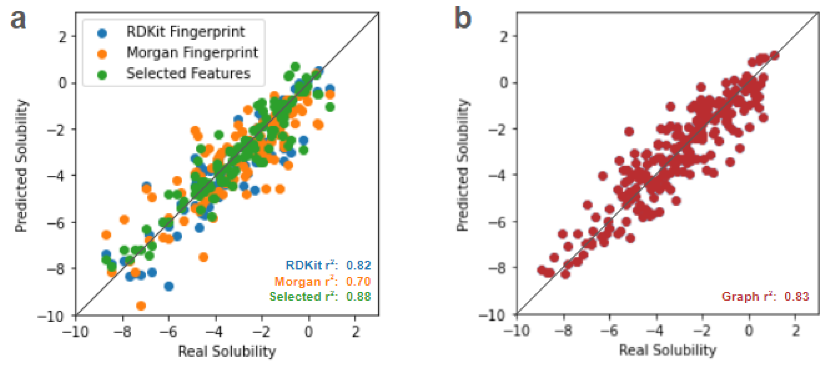
After this data preprocessing, we first begin by testing the performance of three different classical regression methods (linear, ridge, and LASSO) in predicting solubility from each of the three data representations (RDKit fingerprint, Morgan fingerprint, and selected feature vector). Details of these implementations are provided in the Methods section. Parity plots illustrating the performance of these three classical regression techniques on RDKit fingerprints, Morgan fingerprints, and the vector of selected molecular features are shown below in
Figure 1.
The simplest linear regression approach is poorly performant at predicting properties, while ridge regression that penalizes squared magnitudes of coefficients performs slightly better. LASSO regression, which penalizes the magnitudes of coefficients (without squaring), performs better than both, as this approach incorporates the ability to zero out the effect of input predictors and effectively allows for a level of feature selection. (Fonti & Belitser, 2017) For these classical regressors, using a limited vector of selected chemical features that directly represent physical attributes provides better results than the more complicated molecular fingerprints that fully encode each molecule.
However, with the advent of deep learning approaches, one can perform significantly better than the aforementioned classical techniques. Even a naive multilayer perceptron (MLP) approach as in
Figure 2a can be highly performant. The drawback of this MLP approach, however, is that 1)
a priori selection of features is still required for best performance - which is not always possible, especially in the most interesting regimes of novel discovery and 2) the MLP requires training many parameters, in this case around 70,000. Every node of each layer in the model is connected to every node in the subsequent layer, taking a brute force approach to capturing data relationships that may not be needed. Unnecessarily large models can provide a burden on training time, computational resources, and interpretability. And while we are able to implement a minimal 3 layer MLP for the example ESOL dataset used here, this cannot be assumed to be the case for more complex relationships in unknown regimes of novel discovery.
To mitigate MLP issues concerning dependency of input data curation and model size, an alternative deep learning approach is to use graph representations of each molecule. Atoms are represented as nodes and bonds as undirected edges, and a graph convolutional network (GCN) is used to perform graph regression for property prediction, as shown in
Figure 2b. In this way, 1) we do not need to encode
a priori selected features that are relevant to the prediction task and 2) are able to achieve comparable performance to the MLP with a fraction of the parameters, in this case only around 13,000 or <20% of the MLP. Details of MLP and GCN model implementation are provided in the Methods section.
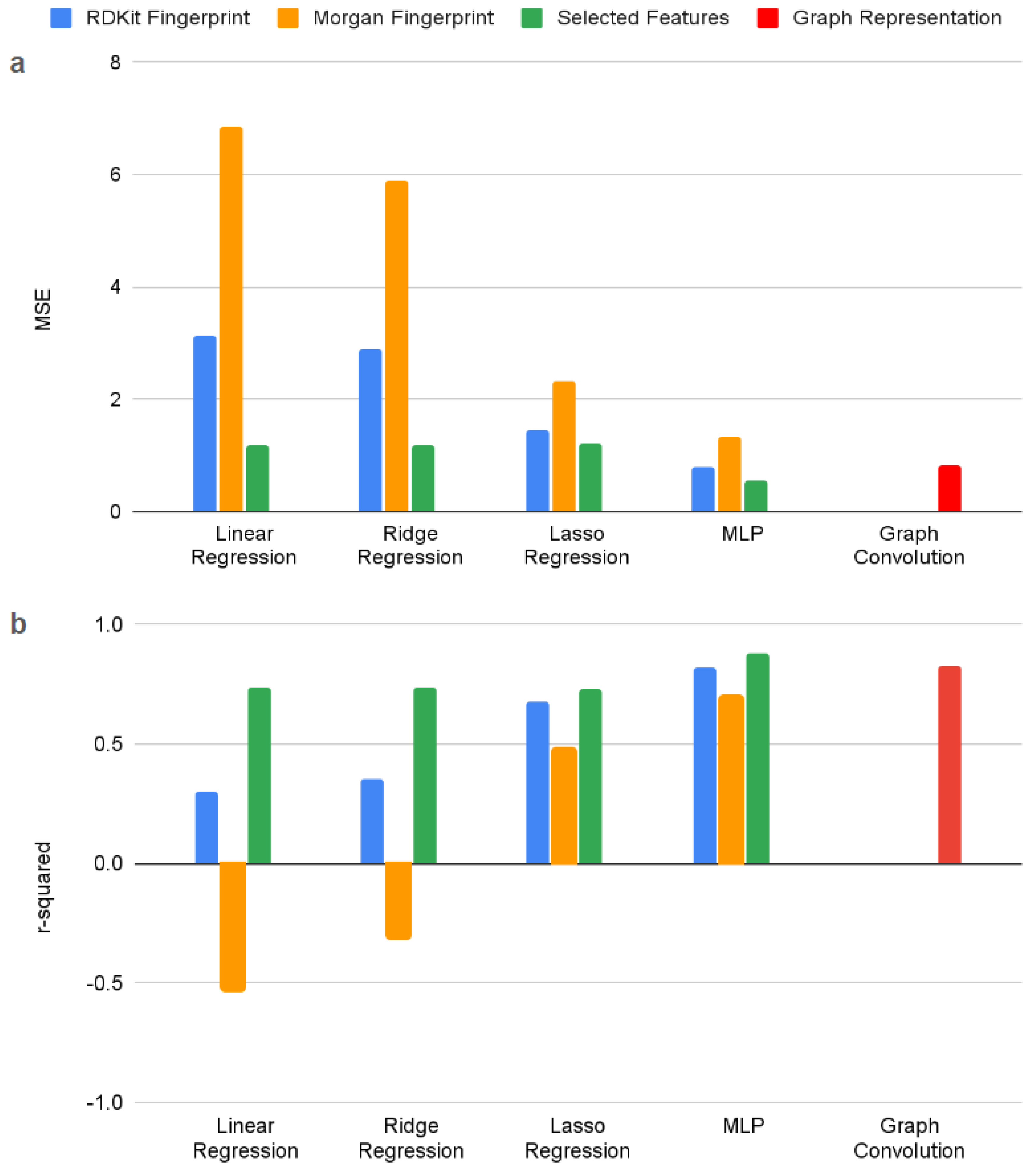
A comparison of the three classic regression techniques (linear, ridge, and LASSO) and the two deep learning techniques (MLP and GCN) is detailed below in
Figure 3. In terms of molecular representation, using selected features performs best, followed by the RDKit fingerprint, and the Morgan fingerprint (which even yields negative r-squared values with linear and ridge regression). In terms of model, the two deep learning approaches, MLP and GCN, are competitive depending on the molecular representation. Then performance is followed by LASSO regression, ridge regression, and basic linear regression.
While the MLP performs best when operating on selected features, the graph approach performs comparable to the MLP on RDKit fingerprints - without needing to preprocess the molecule into a fingerprint or utilize as many parameters. When access to intuitively selected features does not exist (as when attempting to explore unknown structure-property relationships) the graph method offers both high performance and fewer parameters to train, store, and interpret compared to the MLP. As a result, graph networks have been a growing and popular approach for chemical property prediction. (Reiser et al., 2022)
Despite their successes, graph approaches are not perfect. For instance, there is a limit to how deep a GCN can be made - too many layers will make features indistinguishable and hurt classification accuracy. (Li et al., 2018) Additionally, current schemes cannot provably distinguish all distinct graphs up to graph isomorphisms, (Murphy et al., 2019) meaning a GCN approach may spuriously treat different molecules identically in certain circumstances. Thus, we next explore an alternate deep learning approach to solubility prediction.
Previously in
Figure 3, we identified optimal results by applying models on pre-selected features. But, because the manual determination of important features is such an art, we ideally would want to incorporate the ability to learn important relationships between features into the model design. Here, we can pull from interdisciplinary successes in modern language models, which leverage the attention mechanism to excel at processing key relationships within a data string. In short, these attention-based approaches “tokenize” an input and learn the strength of correlations between each token (and its own token in self-attention cases) in order to make a prediction. (Vaswani et al., 2017) In other words, how much each token “pays attention” to each other is determined. Using an attention-based approach, which has been demonstrated to successfully perform tasks such as predicting the overall sentiment from a language string, (Letarte et al., 2018) allows us to analogously predict an overall molecular property from a string representation of molecular structure.
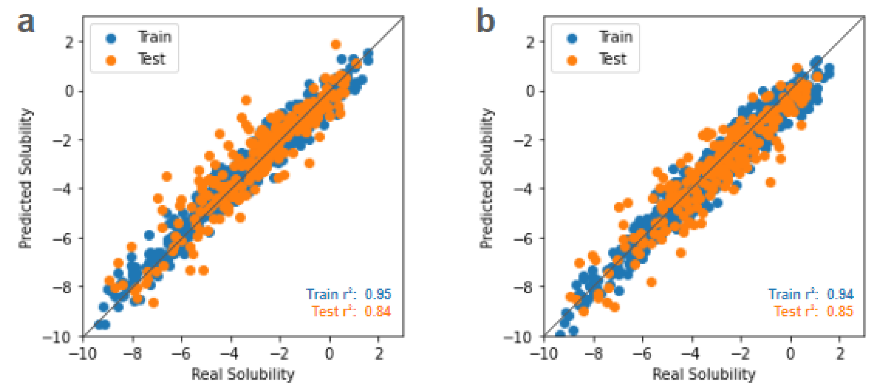
Thus, here we apply an attention-based transformer encoder network to operate directly on SMILES strings and obtain highly performant results without requiring pre-selected features. This model has a more complicated architecture than a simple MLP, with choices for how many attention branches or “heads” to use, how large the embedding dimension is per head, and a dropout parameter acting as a regularization factor. Rather than manually choose values for these hyperparameters by intuition or conduct a brute force guess-and-check search, we subsequently implement Bayesian optimization to systematically tune these hyperparameters of the attention encoder model. Parity plots for the initial transformer model and the Bayesian optimized transformer model are shown in
Figure 4a and 4b, respectively. Details of the transformer model and Bayesian optimization process are provided in the Methods section.
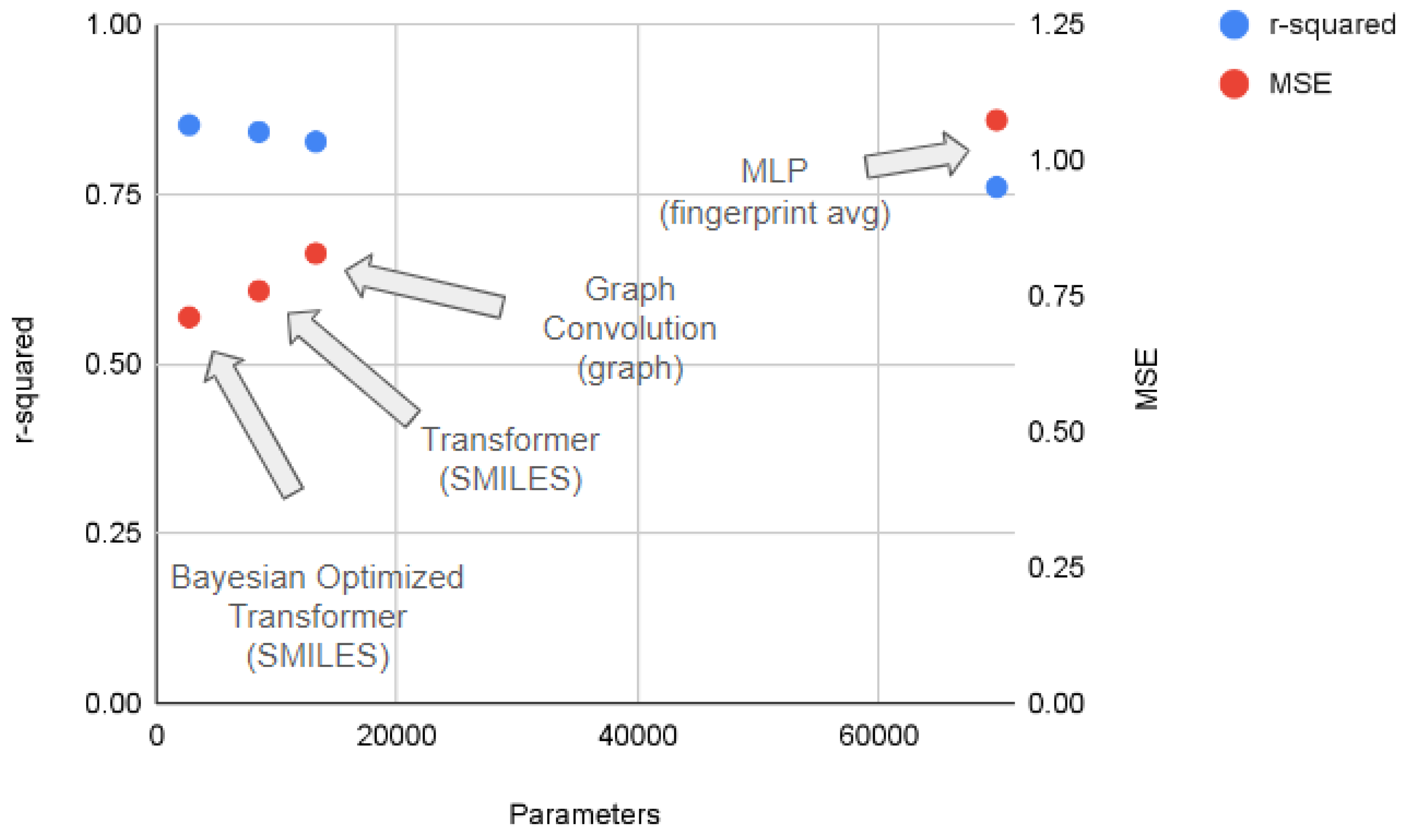
Figure 5 shows a comparison of deep learning approaches operating in the regime of minimal data curation, where pre-selected features are not available. We compare the performance of each approach (in terms of r-squared and MSE values) along with each model size (in terms of number of parameters). Each approach is labeled by both the deep learning model and the molecular representation used.
The performance of the MLP approach (averaged between RDKit and Morgan molecular fingerprints) performs comparably the worst, while also being the most unwieldy model requiring the largest number of parameters. The graph convolutional network approach requires fewer parameters and performs better than the MLP fingerprint average. The attention-based transformer model is even more efficient at learning the relationship between chemical structure and solubility than the graph convolution model, reaching better performance with even fewer parameters. Finally, the Bayesian optimized transformer model simultaneously attains the highest r-squared and the lowest MSE, while requiring the fewest parameters. These results provide an alternative to simply naively increasing the size of a deep learning model to increase performance.
3. Conclusions
The ability to isolate specific factors from the overall molecule, either a priori from chemical intuition or generated during model training, is key to successful property prediction. This is shown both on the data representation side, with the positive performance of using a limited vector of selected features instead of a general molecular fingerprint, and on the simple model selection side with the success of LASSO regression’s feature selection capability over basic linear and ridge regression. Selecting key information from molecular structure simplifies the relationship that must be learned in order to output solubility. When such knowledge of key features exists, it may not be necessary to appeal to more complicated deep learning approaches.
In the absence of knowing beforehand which molecular features map well to a property of interest, deep learning models provide avenues for successful property prediction. Fully connected multilayer perceptrons provide a brute force method of learning the complicated relationship between structure and solubility, which outperforms the simpler non-deep models. Graph convolution models provide a more parameter efficient approach for performant solubility prediction, and utilize an intuitive way of representing chemical structures as atoms and bonds rather than an arguably opaque binary fingerprint. It is thus of little surprise that graph approaches have become popular for chemical analysis.
While graph treatments of chemical property prediction remain common and fruitful, we also demonstrate an alternative approach inspired by modern language processing that is able to act directly on the common SMILES string representation of molecules. Transformer models are used in state-of-the-art language processing tasks and the framework of linguistic sentiment analysis provides a generalizable method for mapping SMILES strings to molecular property. Here, even fewer model parameters are used while attaining better predictive performance, indicating the relationships learned to be encoded by each parameter of the model are more salient than those of the MLP and GCN. As an additional layer of improvement, Bayesian optimization can systematically guide us to fine tune model structure for further improved solubility prediction, without needing to fall back on trial-and-error operator intuition for manually picking “magic numbers” that define the model.
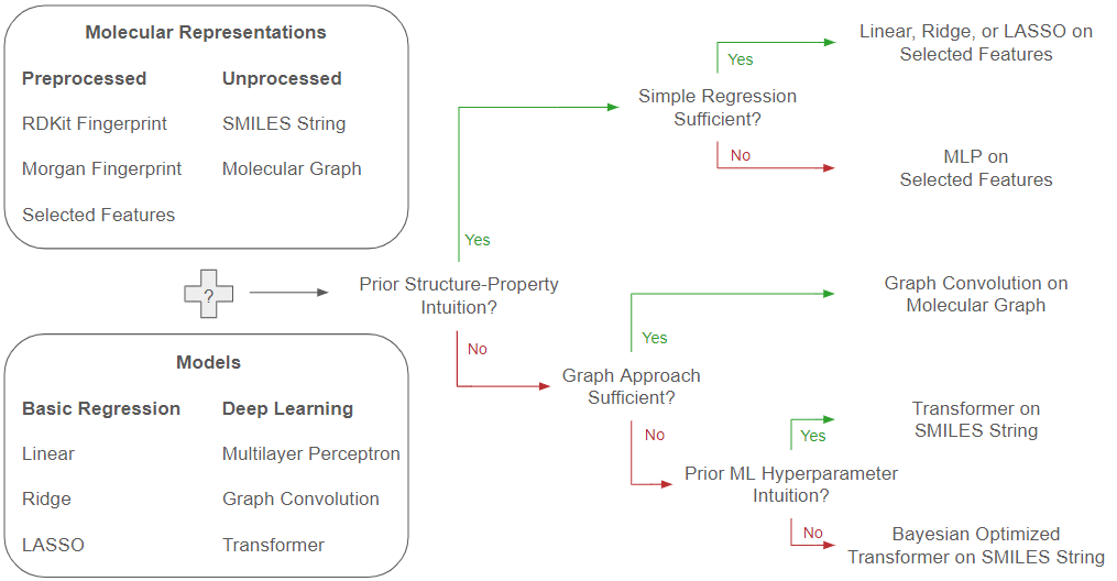
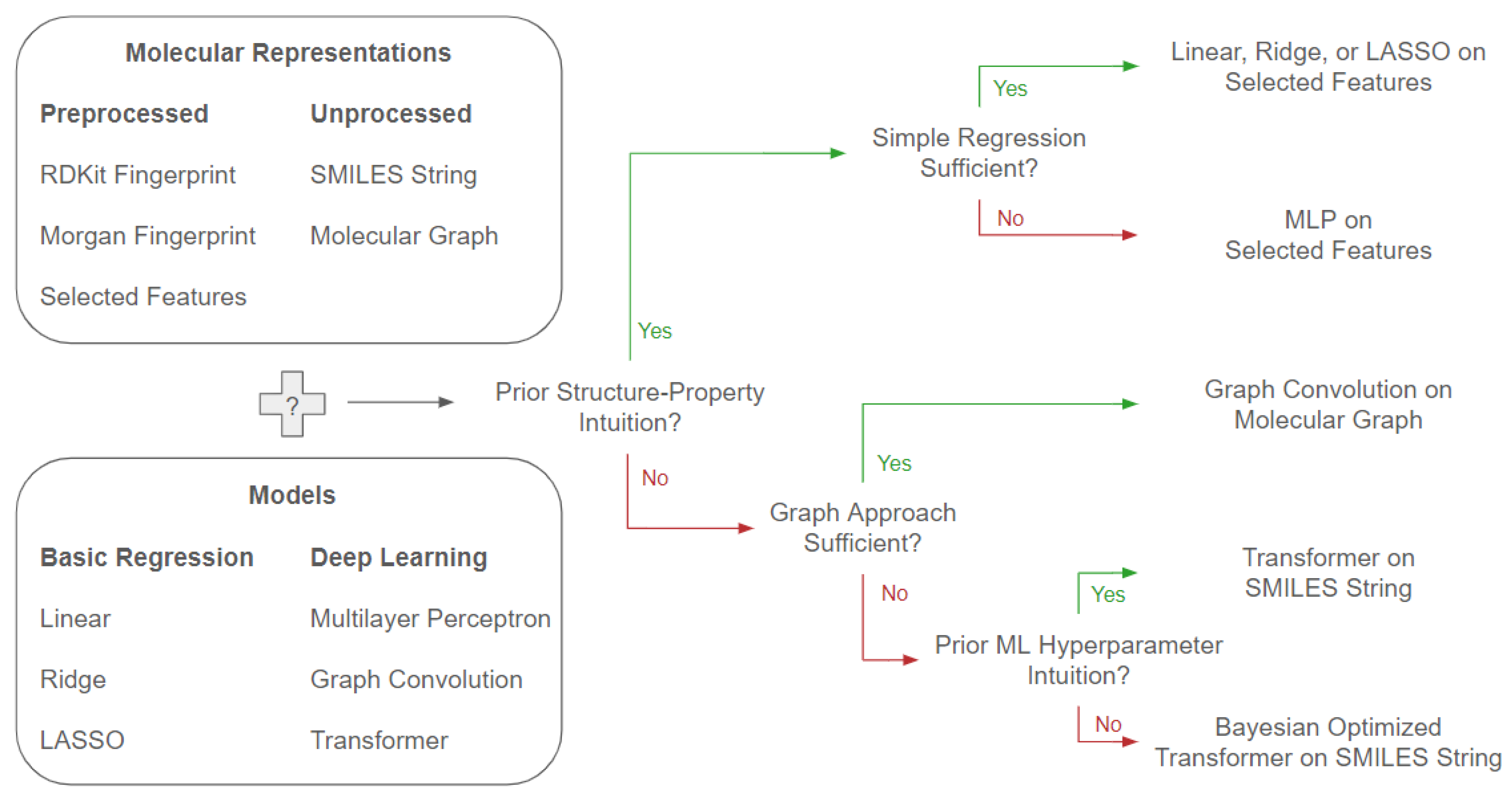
Closing the loop on our initial questions of how to choose both appropriate molecular representations and predictive model approaches for performant property prediction, we summarize a flowchart of choices based off our results in the following
Figure 6.
4. Methods
Dataset Curation
Here we use the MoleculeNet ESOL dataset (Wu et al., 2018) which provides water solubility data (log solubility in mols/L) for common organic small molecules along with various forms of molecular representation.
We use two forms of molecular fingerprinting to obtain representations of structure and similarity, the RDKit fingerprint and the Morgan fingerprint. Both forms used here consist of 512-dimensional vectors. The RDKit fingerprint algorithm identifies all subgraphs in the molecule within a particular range of sizes, hashes the subgraph to obtain a bit ID, and then modifies it to fit into the fingerprint size. (Landrum, 2024) Here, we use the default max path size of 7 bonds. The Morgan fingerprint encodes circular substructures around each atom to help leverage local structure information for property prediction. However, this fingerprint yields a poor perception of global molecular features, including overall size, shape, and larger structural differences. (Capecchi et al., 2020)
Thus, we also represent molecular structures with a 6-dimensional vector of selected overall molecular features which have been considered to have an effect on solubility: molecular weight, (Kubota & Eguchi, 1997) number of atoms, (Tolls et al., 2002) number of heavy atoms, (Frolov & Kiselev, 2014) number of heteroatoms, (Li et al., 2022) topological polar surface area, (Ali et al., 2011) and number of valence electrons. (Seidel et al., 2016)
We organize our three different input molecular representations matched off with respective output solubilities, and split the total dataset into 790 training sets and 112 test sets.
Classic Regression Methods
We implement the simple linear, ridge, and LASSO regression models with the standard scikit-learn python library. (Pedregosa et al., 2011) The objective functions minimized for ridge and LASSO regressions are shown in the below Equations 1 and 2, respectively.
where for both ridge and LASSO regressions, X is the training data, y is the target values, w is the weights, and
is a regularization strength parameter, chosen to be 0.05.
is the shape of target values y. After fitting on the training data, the plotted predictions, mean squared error values, and r-squared are calculated on the test dataset.
Multilayer Perceptron Model
We use PyTorch (Paszke et al., 2017) to implement a basic three layer multilayer perceptron, the minimum size for a “deep” learning framework in which the second layer is hidden from the inputs and outputs.
This model takes in a 512-D molecular fingerprint and outputs a single solubility value, with the architecture used shown below:
MLP(
(dense1): Linear(in_features=512, out_features=128, bias=True)
(dense2): Linear(in_features=128, out_features=32, bias=True)
(out): Linear(in_features=32, out_features=1, bias=True)
)
Number of Parameters: 69825
However, because the selected features vector is only 6-D vs a molecular fingerprint of 512-D, a different model architecture is required in the input layer for application on the selected features case. This second model also required adjusting the size of the output layer in order to be comparable with that of the fingerprint analyses.
These adjustments thus also yield a 3 layer network with approximately 70,000 parameters, with the architecture as shown below:
MLP_f(
(dense1): Linear(in_features=6, out_features=512, bias=True)
(dense2): Linear(in_features=512, out_features=128, bias=True)
(out): Linear(in_features=128, out_features=1, bias=True)
)
Number of Parameters: 69377
Graph Convolution Model
The graph convolution network is also implemented in PyTorch, here utilizing the torch geometric library. (Fey & Lenssen, 2019) The graph convolution model takes in graph representations of molecules in the ESOL dataset, instead of the vectorized fingerprints and features of the previous models, and for each convolution layer merges each node’s features with those of its neighbors. The model outputs a single global embedding, trained to correspond to the molecule’s solubility.
The model architecture for the simple GCN used here is shown below:
GCN(
(initial_conv): GCNConv(9, 64)
(conv1): GCNConv(64, 64)
(conv2): GCNConv(64, 64)
(conv3): GCNConv(64, 64)
(out): Linear(in_features=128, out_features=1, bias=True)
)
Number of Parameters: 13249
Transformer Model
The transformer model is also implemented in PyTorch, and utilizes the multi-headed attention architecture. (Vaswani et al., 2017) Instead of acting on preprocessed molecular representations like fingerprints or intuition-selected features, we use the SMILES strings for each molecule in the ESOL dataset directly. In brief, the model first chunks a SMILES string into tokens and passes these tokens through a positional encoding layer. Then, the attention function passes the positionally encoded embeddings through linear dense layers to form keys, queries, and values for each token. Each token maps its query to the most similar keys of itself and other tokens, and outputs a weighted sum of values based on query-key similarities. Then, the activated values are concatenated and passed through another linear layer.
Multi-headed attention uses multiple sets of attention layers running in parallel, which can all be trained to capture different intertoken relationships. For our initial implementation of the transformer network, we use an embedding size of 32, distributed among 4 attention heads for branches consisting of 8 dimensions each, a dropout factor of 0.1, and train for 3000 epochs. This model architecture is as below:
Encoder(
(embedding): Embedding(34, 32)
(pos_encoder): PositionalEncoding(
(dropout): Dropout(p=0.1, inplace=False)
)
(self_attention): MultiHeadAttention(
(W_q): Linear(in_features=32, out_features=32, bias=True)
(W_k): Linear(in_features=32, out_features=32, bias=True)
(W_v): Linear(in_features=32, out_features=32, bias=True)
(W_o): Linear(in_features=32, out_features=32, bias=True)
)
(linear): Linear(in_features=3136, out_features=1, bias=True)
(norm): LayerNorm((32,), eps=1e-05, elementwise_affine=True)
(dropout): Dropout(p=0.1, inplace=False)
)
Number of Parameters: 8513
Bayesian Optimization of Hyperparameters
The basic hyperparameters governing the attention-based transformer encoder network that we explore here are: the number of attention heads, the embedding dimension per head, and the dropout percent. (PyTorch Contributors, 2023) Bayesian optimization acts to navigate a search space toward minimizing a given objective function, using a surrogate function that approximates the search space and an acquisition function that scores exploration choices. Here, our search space is a 3-D space spanned by our selection of hyperparameters, the objective function is the loss of the model when trained with those hyperparameters, the surrogate function is the commonly used Gaussian process, and the acquisition function is probability of improvement. The probability of improvement is calculated as shown in the below Equation 3:
where
is the cumulative distribution function,
and
are the mean and standard deviation of the surrogate Gaussian process sampled at a new choice of hyperparameters x, and
is the surrogate evaluated at the best hyperparameter configuration sampled so far.
To expedite exploration of hyperparameter space, for the objective function we initially restrict training to only 200 epochs instead of the 3000 epochs originally used. After identifying the optimally performing set of hyperparameters in this small scale, we then train that model to convergence with the full 3000 epochs. Specifically, we identify a model created with 1 head, 14 dimensions per head, and 0.029 dropout performs the best, while using less than 1/3 of the parameters (2717 vs 8513) of the original non-optimized attention model.
Author Contributions
Conceptualization, A.J.L., project administration, A.J.L., writing – original draft preparation, A.J.L. writing – review and editing, A.J.L. All authors have read and agreed to the published version of the manuscript.
Funding
This work received no external funding.
Acknowledgements
The author thanks Audrey Lai for assistance in the editing process.
Conflicts of Interest
The author declares no conflicts of interest.
References
- Ali, J., Camilleri, P., Brown, M. B., Hutt, A. J., & Kirton, S. B. (2011). Revisiting the General Solubility Equation: In Silico Prediction of Aqueous Solubility Incorporating the Effect of Topographical Polar Surface Area. Journal of Chemical Information and Modeling, 52(2). [CrossRef]
- Ba, J., & Caruana, R. (2014). Do deep nets really need to be deep? Advances in neural information processing systems, 27.
- Capecchi, A., Probst, D., & Reymond, J.-L. (2020). One molecular fingerprint to rule them all: drugs, biomolecules, and the metabolome. Journal of Cheminformatics, 12(43). [CrossRef]
- Chen, H., Kogej, T., & Engkvist, O. (2018). Cheminformatics in drug discovery, an industrial perspective. Molecular Informatics, 37(1800041), 9-10. [CrossRef]
- Fey, M., & Lenssen, J. E. (2019). Fast graph representation learning with PyTorch Geometric. arXiv preprint, arXiv:1903.02428. [CrossRef]
- Fonti, V., & Belitser, E. (2017). Feature selection using lasso. VU Amsterdam research paper in business analytics, 30, 1-25.
- Frolov, A. I., & Kiselev, M. G. (2014). Prediction of Cosolvent Effect on Solvation Free Energies and Solubilities of Organic Compounds in Supercritical Carbon Dioxide Based on Fully Atomistic Molecular Simulations. The Journal of Physical Chemistry B, 118(40). [CrossRef]
- Gomez, L. (2018). Decision Making in Medicinal Chemistry: The Power of Our Intuition. ACS Medicinal Chemistry Letters, 9(10), 956−958. [CrossRef]
- Kubota, N., & Eguchi, Y. (1997). Facile Preparation of Water-Soluble N-Acetylated Chitosan and Molecular Weight Dependence of Its Water-Solubility. Polymer Journal, 29(2), 123-127. [CrossRef]
- Landrum, G. (2024). RDKit: Open-source cheminformatics. https://www.rdkit.org. [CrossRef]
- Letarte, G., Paradis, F., Giguère, P., & Laviolette, F. (2018). Importance of Self-Attention for Sentiment Analysis. Proceedings of the 2018 EMNLP Workshop BlackboxNLP: Analyzing and Interpreting Neural Networks for NLP, 267-275.
- Lew, A. J. (2023). Elucidating Structure-Property Relationships for Targeted Materials Mechanical Design. Massachusetts Institute of Technology. https://dspace.mit.edu/handle/1721.1/150564.
- Lew, A. J., & Buehler, M. J. (2021). A deep learning augmented genetic algorithm approach to polycrystalline 2D material fracture discovery and design. Applied Physics Reviews, 8, 041414. [CrossRef]
- Lew, A. J., & Buehler, M. J. (2021). Encoding and exploring latent design space of optimal material structures via a VAE-LSTM Model. Forces in Mechanics, 5, 100054. [CrossRef]
- Lew, A. J., & Buehler, M. J. (2022). DeepBuckle: Extracting physical behavior directly from empirical observation for a material agnostic approach to analyze and predict buckling. Journal of the Mechanics and Physics of Solids, 164, 104909. [CrossRef]
- Lew, A. J., & Buehler, M. J. (2023). Single-shot forward and inverse hierarchical architected materials design for nonlinear mechanical properties using an attention-diffusion model. Materials Today, 64, 10-20. [CrossRef]
- Lew, A. J., Jin, K., & Buehler, M. J. (2023). Designing architected materials for mechanical compression via simulation, deep learning, and experimentation. npj Computational Materials, 9(1), 80. [CrossRef]
- Lew, A. J., Stifler, C. A., Cantamessa, A., Tits, A., Ruffoni, D., Gilbert, P. U.P.A., & Buehler, M. J. (2023). Deep learning virtual indenter maps nanoscale hardness rapidly and non-destructively, revealing mechanism and enhancing bioinspired design. Matter, 6(6), 1975-1991. [CrossRef]
- Lew, A. J., Yu, C.-H., Hsu, Y.-C., & Buehler, M. J. (2021). Deep learning model to predict fracture mechanisms of graphene. npj 2D Materials and Applications, 5(1), 48. [CrossRef]
- Li, K., Hu, J.-M., Qin, W.-M., Guo, K., & Cai, Y.-P. (2022). Precise heteroatom doping determines aqueous solubility and self-assembly behaviors for polycyclic aromatic skeletons. Communications Chemistry, 5(104). [CrossRef]
- Li, Q., Han, Z., & Wu, X.-M. (2018). Deeper Insights into Graph Convolutional Networks for Semi-Supervised Learning. The Thirty-Second AAAI Conference on Artificial Intelligence (AAAI-18), 32(1). [CrossRef]
- Liu, Y., Zhao, T., Ju, W., & Shi, S. (2017). Materials discovery and design using machine learning. Journal of Materiomics, 3(3), 159-177. [CrossRef]
- Murphy, R. L., Srinivasan, B., Rao, V., & Ribeiro, B. (2019). Relational Pooling for Graph Representations. arXiv preprint, arXiv:1903.02541v2 [cs.LG]. [CrossRef]
- Niazi, S. K. (2023). The Coming of Age of AI/ML in Drug Discovery, Development, Clinical Testing, and Manufacturing: The FDA Perspectives. s, Drug Design, Development and Therapy, 2691-2725. [CrossRef]
- Paszke, A., Gross, S., Chintala, S., Chanan, G., Yang, E., DeVito, Z., Lin, Z., Desmaison, A., Antiga, L., & Lerer, A. (2017). Automatic differentiation in pytorch. 31st Conference on Neural Information Processing Systems. https://openreview.net/pdf?id=BJJsrmfCZ.
- Paul, D., Sanap, G., Shenoy, S., Kalyane, D., Kalia, K., & Tekade, R. K. (2020). Artificial intelligence in drug discovery and development. Drug Discovery Today, 26(1), 80-93. [CrossRef]
- Pedregosa, F., Varoquaux, G., Gramfort, A., Michel, V., Thirion, B., Grisel, O., Blondel, M., Prettenhofer, P., Weiss, R., Dubourg, V., & Vanderplas, J. (2011). Scikit-learn: Machine learning in Python. Journal of Machine Learning Research, 12, 2825-2830.
- Pollice, R., Passos Gomes, G. d., Aldeghi, M., Hickman, R. J., Krenn, M., Lavigne, C., Lindner-D'Addario, M., Nigam, A., Ser, C. T., Yao, Z., & Aspuru-Guzik, A. (2021). Data-Driven Strategies for Accelerated Materials Design. Accounts of Chemical Research, 54(4). [CrossRef]
- PyTorch Contributors. (2023). Transformer — PyTorch 2.4 documentation. PyTorch. Retrieved September 8, 2024, from https://pytorch.org/docs/stable/generated/torch.nn.Transformer.html.
- Reiser, P., Neubert, M., Eberhard, A., Torresi, L., Zhou, C., Shao, C., Metni, H., Hoesel, C. v., Schopmans, H., Sommer, T., & Friederich, P. (2022). Graph neural networks for materials science and chemistry. Communications Materials, 9(93). [CrossRef]
- Sanchez-Lengeling, B., & Aspuru-Guzik, A. (2018). Inverse molecular design using machine learning: Generative models for matter engineering. Science, 361(6400), 360-365. [CrossRef]
- Seidel, R., Winter, B., & Bradforth, S. E. (2016). Valence Electronic Structure of Aqueous Solutions: Insights from Photoelectron Spectroscopy. Annual Review of Physical Chemistry, 67, 283-305. [CrossRef]
- Sertkaya, A., Beleche, T., & Jessup, A. (2024). Costs of Drug Development and Research and Development Intensity in the US, 2000-2018. JAMA Netw Open, 7(6), e2415445. [CrossRef]
- Tolls, J., Dijk, J. v., Verbruggen, E. J.M., Hermens, J. L.M., Loeprecht, B., & Schuurmann, G. (2002). Aqueous Solubility−Molecular Size Relationships: A Mechanistic Case Study Using C10- to C19-Alkanes. The Journal of Physical Chemistry A, 106(11), 2760-2765.
- Vaswani, A., Shazeer, N., Parmar, N., Uszkoreit, J., Jones, L., Gomez, A. N., Kaiser, L., & Polosukhin, I. (2017). Attention Is All You Need. arXiv preprint, arXiv:1706.03762. [CrossRef]
- Weininger, D. (1988). SMILES, a chemical language and information system. 1. Introduction to methodology and encoding rules. Journal of Chemical Information and Computer Sciences, 28(1), 31-36. [CrossRef]
- Wu, Z., Ramsundar, B., Feinberg, E. N., Gomes, J., Geniesse, C., Pappu, A. S., Leswing, K., & Pande, V. (2018). MoleculeNet: a benchmark for molecular machine learning. Chemical science, 9(2), 513-530. [CrossRef]
|
Disclaimer/Publisher’s Note: The statements, opinions and data contained in all publications are solely those of the individual author(s) and contributor(s) and not of MDPI and/or the editor(s). MDPI and/or the editor(s) disclaim responsibility for any injury to people or property resulting from any ideas, methods, instructions or products referred to in the content. |
© 2024 by the authors. Licensee MDPI, Basel, Switzerland. This article is an open access article distributed under the terms and conditions of the Creative Commons Attribution (CC BY) license (http://creativecommons.org/licenses/by/4.0/).
