Introduction
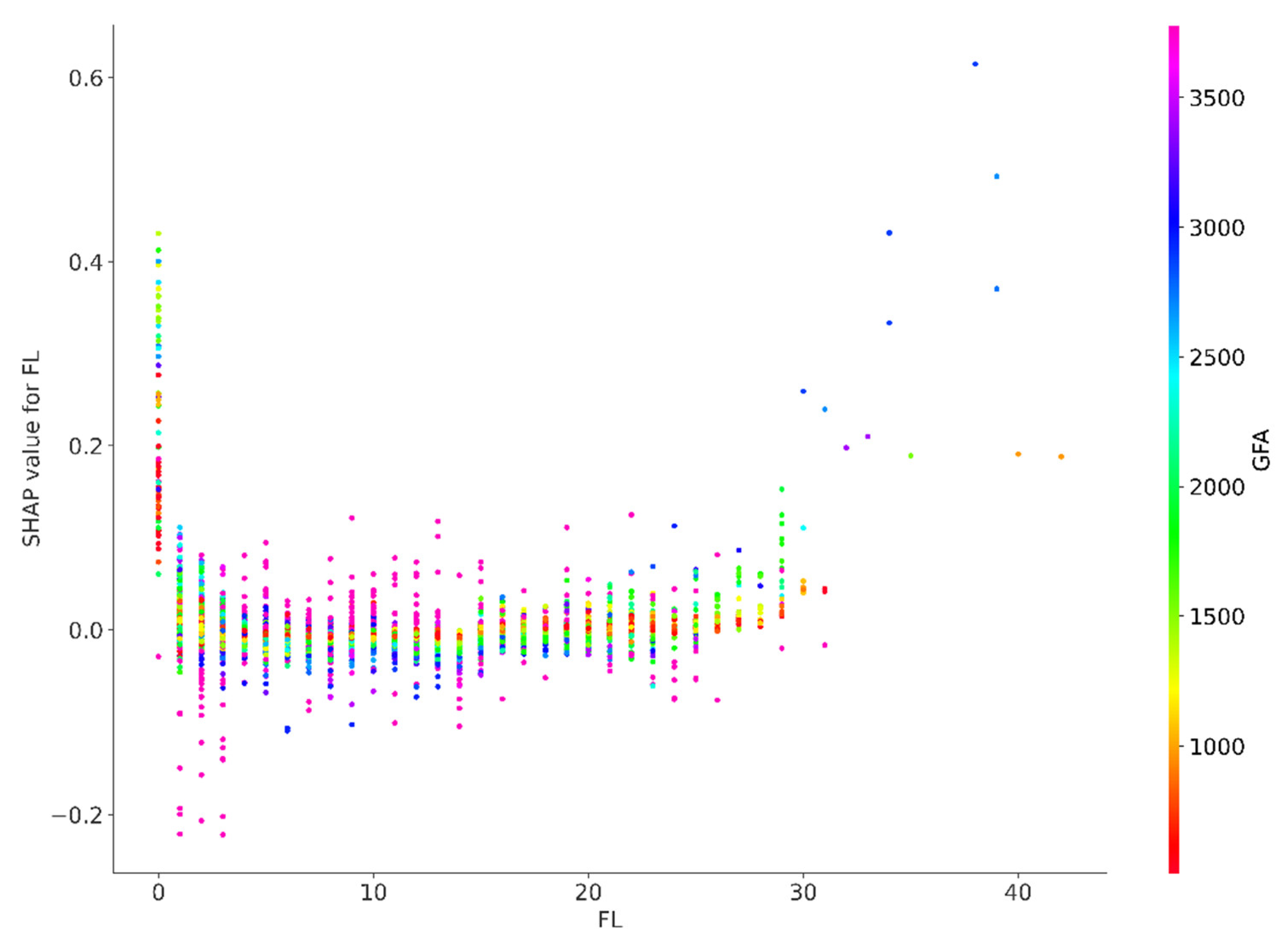
The Hong Kong industrial property market has long been a subject of fascination and scrutiny, given its significant contributions to the city’s economy. First, a distinctive characteristic of the Hong Kong industrial property market is the price premium commanded by properties at lower floor levels. In contrast to residential properties, where higher floor levels typically offer more desirable views and living conditions, lower–floor industrial properties, especially those on ground floor, are valued more highly due to their proximity to loading and unloading points for container trucks. Businesses may be reluctant to pay premium prices for units with higher logistical costs, leading to lower prices for higher–floor units. This peculiarity has significant implications for property developers, investors, and occupiers who must navigate the complexities of industrial property pricing to make informed decisions.
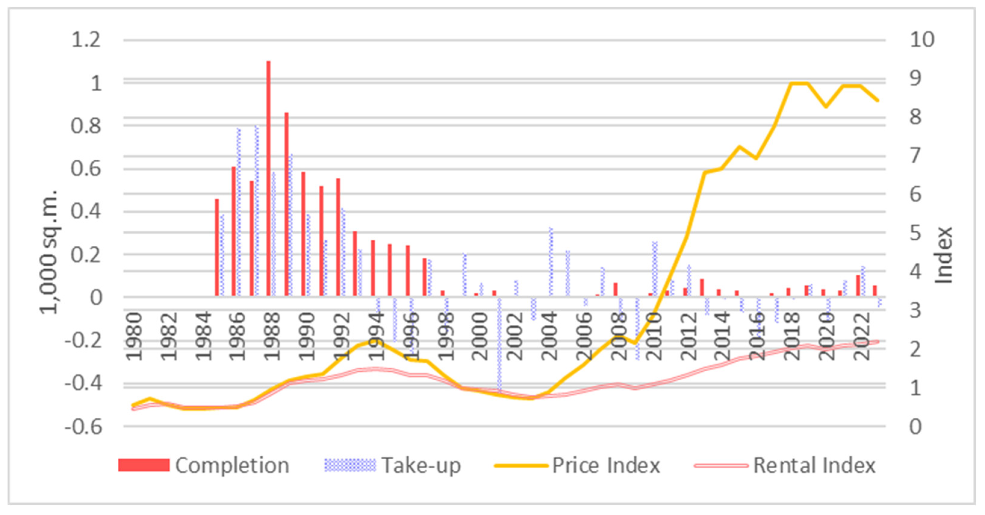
Second, the industrial property sector has exhibited a paradoxical phenomenon, where property developers have consistently produced large volumes of new industrial accommodations despite the longstanding trend of de–industrialization that began in the late 1970s. Hong Kong’s transformation from a low–cost, labour–intensive manufacturing base to a world–class financial and business centre has been a gradual process over the past six decades (Tang and Ho, 2014). Although manufacturing accounted for roughly 1% of GDP in 2021 (Hong Kong SAR Government, 2023), industrial accommodations have remained the second largest stock of floor space in the city, following residential properties. As reported by the Rating and Valuation Department (2024), in 2022, residential properties accounted for 62.84% of the total floor area, measuring 96.61 million square metres. This was followed by industrial properties at 16.79%, commercial properties at 12.10%, storage facilities at 3.95%, specialized factories at 3.40%, industrial/office mixed–use properties at 0.55%, and office spaces at 0.36%.
This apparent contradiction between industrial property development and de–industrialization can be attributed to various factors, including the entrepreneurial decisions of local industrialists (Yeh and Ng, 1994), government policies (Sit, 1995), and changing global economic conditions. The manufacturing sector, once the driving force behind the economy, has undergone significant contraction since the late 1980s. The labor–intensive and low–cost manufacturing sector, which was prominent in the 1970s and 1980s, has been steadily shrinking in terms of employment and its contribution to GDP (Yeh, 1997). The number of manufacturing sector employees grew from approximately 766,230 persons in the first quarter of 1978 to around 942,820 persons in the second quarter of 1981. However, this figure subsequently declined to 91,800 persons in the fourth quarter of 2022 (Census and Statistics Department, 2024). The income share of the manufacturing sector as a percentage of GDP reached its peak at 28.3% in 1979, fell to 6% in 1998 and fell further to 1% in 2021 (Census and Statistics Department, 2013; Hong Kong SAR Government, 2023).
The majority of these industrial buildings are general–purpose industrial sheds, developed by property developers for sale or lease to individual occupiers, who can utilize them for a range of non–polluting manufacturing activities, including non–specialist warehousing and storage (Tang and Ho, 2014). This persistence of property development in this sector is noteworthy, particularly during the period between 1980 and 1997, when the trend of de–industrialization appeared to be irreversible. A possible explanation for this phenomenon lies in indirect evidence suggesting that these premises were used for industrial support functions and various office activities, such as administration, marketing, and packaging, which were not permitted under the prevailing planning regulations (Chau and Chan, 2008).
Moreover, the city’s property developers continued to produce new industrial space due to the growing demand for non–industrial activities from the office sector. This demand was driven by the increasing need for flexible and adaptable workspaces, which industrial properties could accommodate (Adams 1990; Wood and Williams, 1992). The blurring of boundaries between industrial and office uses has led to a more complex property market, where industrial properties are being repositioned to meet the changing needs of occupiers (Daniels and Bryson, 2002).
This phenomenon is further underscored by the observation that new industrial space production continued at a high level throughout the 1980s and into the mid–1990s, maintaining industrial rents at a relatively low and stable level compared to lower–grade offices. This suggests that the demand for industrial space was not only driven by manufacturing activities but also by other non–industrial uses, such as warehousing and storage (Tang and Ho, 2015).
In response to rapid development pressure and economic restructuring, the government has commissioned various planning studies on redeveloping obsolete industrial properties since the 1980s. However, government decisions to permit non–manufacturing uses in industrial premises were slow and incremental, reflecting a rigid bureaucratic approach to demarcating industrial and office uses. Since the mid–1990s, incremental policies have been implemented to relax development control restrictions, introduce new industrial land–use zones, and encourage adaptive re–use (Kee, et al., 2019; Kee and Chau, 2020) or more flexible uses of obsolete industrial space (Development Bureau, 2010).
This paper aims to elucidate the complex dynamics governing industrial property prices in Hong Kong using advanced machine learning techniques. Specifically, we utilize Explainable AI (XAI) methods (Lundberg, et al., 2018), including Gradient Boosting Machines (GBM) and Shapley value analysis (Shapley, 1953), to identify the primary drivers of industrial property prices and provide valuable insights into the interplay between property characteristics, location, and market conditions. By leveraging these advanced machine learning methods, we aim to contribute to the limited knowledge on industrial property markets in Hong Kong, and present a novel approach to understanding this intricate and dynamic market.
This paper is organized into five sections, which provide a comprehensive examination of the research methodology and findings. Section 2 presents a thorough review of the existing literature on machine learning algorithms, with a particular focus on Gradient Boosting Machines and Shapley values, as well as their applications in real estate valuation. Section 3 delves into the methodology employed in this study, providing a detailed exposition of the theoretical foundations of Shapley values, their application in decision–making under uncertainty, and their potential utilization in measuring the relative importance of each feature in predicting a given property price. Section 4 presents the results of our analysis, accompanied by an interpretation of their implications for understanding the Hong Kong industrial property market. This section aims to provide insights into the complex dynamics governing industrial property prices in Hong Kong, shedding light on the factors that drive these prices and their impact on the market. Finally, Section 5 concludes with a summary of our findings, highlighting their relevance to the field of real estate research. The paper’s conclusions are drawn from an examination of the data and analysis, providing a comprehensive understanding of the Hong Kong industrial property market and its intricacies.
Literature Review
The application of machine learning algorithms, particularly gradient boosting machines, has become increasingly popular in the field of real estate prediction. This trend is driven by the ability of these algorithms to capture complex relationships between features and provide accurate predictions. One of the key advantages of gradient boosting machines (Friedman, 2001) is their ability to handle large datasets and high–dimensional spaces, making them well–suited for real estate prediction tasks. This literature review aims to explore the use of GBM in predicting real property prices and the employment of Shapley value to enhance model transparency.
Several studies have utilized GBM to predict real property prices. Ho et al. (2021) employ a trio of machine learning algorithms, including support vector machine (SVM), random forest (RF), and gradient boosting machine (GBM), to predict residential property prices in Hong Kong and find that RF and GBM outperform SVM in terms of predictive power and error minimization. Sharma, et al. (2023) implement various machine learning algorithms, including Linear Regression (LR), GBM, Histogram Gradient Boosting Regressor, and Random Forest (RF) Regressor, and found that GBM generated high accuracy.
Almaslukh (2020) propose an optimized model based on the GBM method for housing price prediction and achieved a root mean square error of 0.01167, outperforming other baseline machine learning models. Depner et al. (2023) use GBM to examine the accuracy and bias of market valuations in the U.S. commercial real estate sector, and find that it could capture structured variation in market values.
However, machine learning models are often criticized for their lack of transparency, making it difficult to understand how they arrive at their predictions (Lenaers and de Moor, 2023). To address this issue, several studies have employed Shapley value–based methods to enhance model transparency. Neves, et al. (2024) use SHapley Additive exPlanations (SHAP) to clarify the influence of each feature on price estimates and foster enhanced accountability and trust in AI–driven real estate analytics. Lenaers and de Moor (2023) present a comparative study of six global XAI techniques on a CatBoost model for Belgian residential rent prediction and find that multiple techniques are necessary to comprehensively understand rents drivers.
In conclusion, gradient boosting machine has been widely used in predicting real property prices due to its ability to handle complex relationships between features and provide accurate predictions. However, the lack of transparency in machine learning models has raised concerns about accountability and trust. The use of Shapley value–based methods, such as SHAP, has been shown to enhance model transparency and foster trust in AI–driven real estate analytics. Future research should continue to explore the application of machine learning algorithms in real estate price prediction and the development of more transparent machine learning models.
Methodology
Gradient boosting represents a sophisticated machine learning methodology that constructs a robust predictive model through the aggregation of multiple weak prediction models, predominantly decision trees. The fundamental principle underpinning this technique is the transformation of a weak learner—a model exhibiting suboptimal performance in predicting the outcome variable Y—into a strong learner. In each iteration, the boosting algorithm assigns uniform weights to all observations, with the primary objective of minimizing the discrepancies between the weak learner’s predictions and the actual values. The gradient boosting algorithm leverages the error rate to compute the gradient of the loss function, subsequently utilizing this gradient to ascertain the optimal adjustments to the model parameters at each iteration. This iterative process is executed m times, where m represents a hyperparameter predetermined by the data scientist. The target variable Y is presumed to be a continuous, real–valued quantity. The objective of this approach is to construct an approximation to the weighted summation of functions derived from weak learners The methodology’s efficacy stems from its ability to incrementally refine predictions through the sequential addition of weak learners, each addressing the residual errors of its predecessors. This process, guided by the gradient of the loss function, facilitates the development of a highly accurate composite model capable of capturing complex, non–linear relationships within the data.
Equation (2) is utilized to seek an approximation that minimizes the average value of the loss function over the training set, and commence with a model comprising a constant function, and subsequently transform it into Equation (3):
represents a base learner function where
h denotes the optimal function at each step. However, it is not feasible to precisely determine the optimal function
h that minimizes the loss function
L, as noted by Swathi and Shravani (2019). To address this minimization problem, data scientists can utilize a steepest descent approach. Under the assumption that
is the set of arbitrary differentiable functions on ℝ, the model can be updated according to the following equations:
where the derivatives are taken with respect to the functions
for
is the step length.
While this methodology offers a viable approach to the minimization problem, it is imperative to recognize that the estimation of a GBM inherently yields an approximation rather than an exact solution. The efficacy of the model can be rigorously assessed through a comprehensive evaluation framework encompassing multiple performance metrics. Primarily, the coefficient of determination
calculated for the test set provides a quantitative measure of the model’s explanatory power. This metric elucidates the proportion of variance in the dependent variable that is predictable from the independent variables. Furthermore, a suite of error metrics offers nuanced insights into the model’s predictive accuracy. First, Mean Absolute Error (MAE) quantifies the average magnitude of errors in a set of predictions, without considering their direction. Second, Mean Squared Error (MSE) penalizes larger errors more heavily by squaring the errors before averaging, providing sensitivity to outliers. Third, Mean Absolute Percentage Error (MAPE) expresses accuracy as a percentage, offering a relative measure of prediction accuracy. Fourth, Root Mean Squared Error (RMSE) as the square root of the MSE, this metric provides a measure of the standard deviation of the residuals, maintaining the same units as the response variable. The collective analysis of these metrics facilitates a comprehensive evaluation of the model’s performance, enabling researchers to ascertain its predictive capabilities and limitations within the context of the specific problem domain.
where
and
represent the predicted value and actual value of the target variable
Y, respectively; and
m represents the number of observations in the test data.
Properly tuned hyperparameters can significantly improve a model’s accuracy, efficiency, and robustness, enabling it to better capture the underlying patterns in the data and make more reliable predictions. The hyperparameters associated with the model can be optimized using Optuna to further enhance the accuracy of the model. Kee and Ho (2024) have demonstrated that Optuna completes the hyperparameter tuning process not only 5.58 to 70.50 times more rapidly than the random search and grid search when applied to Random Forest and Gradient Boosting Machine algorithms, but also achieved superior performance in terms of standard evaluation metrics on the test set. Optuna is a powerful Bayesian optimization library in Python that can be used to tune hyperparameters of machine learning models. It uses a probabilistic approach to search for the optimal hyperparameters, which is based on Bayesian inference.
When using Optuna, we define an objective function that evaluates the performance of the model with different hyperparameters. Then, Optuna creates a prior distribution over the hyperparameter space and iteratively samples from the prior distribution and evaluates the objective function for each set of hyperparameters. The posterior distribution is updated based on the observed performance, and the process is repeated until convergence or a stopping criterion is reached. Hyperparameters are essential to determine the performance and ability to generalize of machine learning models.
In the final step, this study employs the SHapley Additive exPlanations (SHAP) technique (SHAP, 2018), a cutting–edge method in Explainable Artificial Intelligence (XAI). SHAP is grounded in Shapley values (Shapley, 1953), a concept rooted in cooperative game theory that provides a consistent and locally accurate approach to interpreting model predictions (Lundberg, et al., 2020). The Shapley value is employed to fairly allocate the cumulative gain or payoff among the constituent features. In the context of machine learning, the features are regarded as the players in game theory, and the prediction output by the model serves as the payoff. The Shapley value ensures that each feature’s contribution to the prediction is precisely accounted for, thereby providing a fair representation of their relative importance.
To compute the Shapley values, we employ the TreeExplainer, which complies with the axioms of additive feature attribution methods, which can be mathematically formalized as:
where
denotes the model’s prediction for the instance .
denotes the average prediction across all instances in the dataset (baseline value).
denotes the Shapley value representing the contribution of feature to the prediction.
The Shapley value
for feature
is computed using the equation (11):
where
denotes the set of all features.
denotes a subset of features not including subset .
denotes the value function (the model prediction using features in subset .)
This formula encompasses all possible permutations of features, thereby ensuring a rigorous allocation of the prediction to each feature in accordance with its relative contribution.
Data Definitions and Sources
The dataset for our study initially encompasses 43,530 transaction records from 822 industrial buildings in Hong Kong, covering the period from January 2010 to September 2022. However, upon rigorous examination, we have identified and subsequently excluded over 2,000 property transactions involving resales, as well as numerous entries with missing values for features such as gross floor area. This refinement process results in a reduced sample of 38,699 observations from 777 industrial buildings. To enhance the robustness of our analysis and mitigate the influence of outliers and potential data errors, we employ a trimming technique. Specifically, we remove the 5% of observations with the lowest and highest transaction prices. This data cleaning procedure yields a final dataset comprising 34,829 cross–sectional and inter–temporal observations from 680 industrial buildings.
The dataset contains detailed information on individual industrial properties, including their locations, transaction dates, occupation permits, sale prices, square footage, floor levels, and other pertinent characteristics (e.g., the inclusion of parking spaces and common areas). This comprehensive data is maintained by the government and compiled by a commercial entity known as “EPRC.” To account for inflationary effects, we have adjusted the industrial property prices in our analysis using the industrial property price index published by the Rating and Valuation Department of the Hong Kong SAR Government. This adjustment ensures that our price comparisons across different time periods are meaningful and reflect real changes in property values. Our data definitions are as follows:
represents the transaction price of industrial buildings measured in HK$ million which is deflated by the official industrial property price index published by the Rating and Valuation Department, HKSAR.
represents the gross floor area measured in square feet.
represents the property age at the time of the transaction which can be measured by the difference between the date of issue of the occupation permit and the date of transaction.
represents the floor level of an industrial property.
is a dummy variable that equals 1 if an industrial property is located at the ground floor, 0 otherwise.
is a dummy variable that equals 1 if an industrial property is sold with a storeroom, 0 otherwise.
represents the number of carparks sold with an industrial property.
is a dummy variable that equals 1 if the common area associated with an industrial property that is managed by its owner, 0 otherwise.
represents the walking time from the property to the nearest MTR station measured in minutes.
and are a dummy variable that equals 1 if an industrial property is located at the specific location, 0 otherwise.
Exploratory Data Analysis
Exploratory data analysis (EDA) is a crucial preliminary step in statistical research, focusing on the examination and summarization of datasets to uncover patterns, trends, and characteristics prior to formal modeling or hypothesis testing. This approach employs both graphical and numerical methods to provide researchers with comprehensive insights into key data attributes. In our study, we utilize various EDA techniques to analyze property prices and associated features.
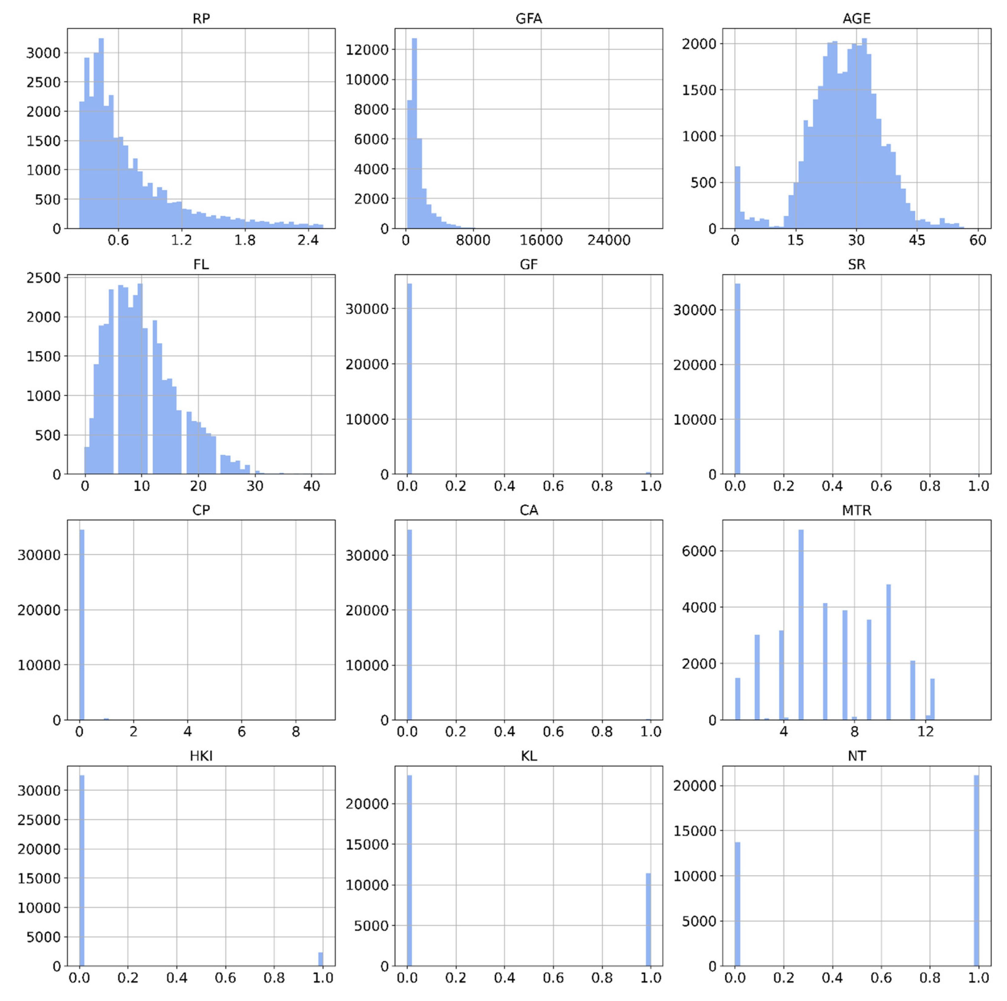
Figure 1 presents histograms for each feature, offering approximate evaluations of their probability distributions by displaying the frequencies of observations within specific value ranges.
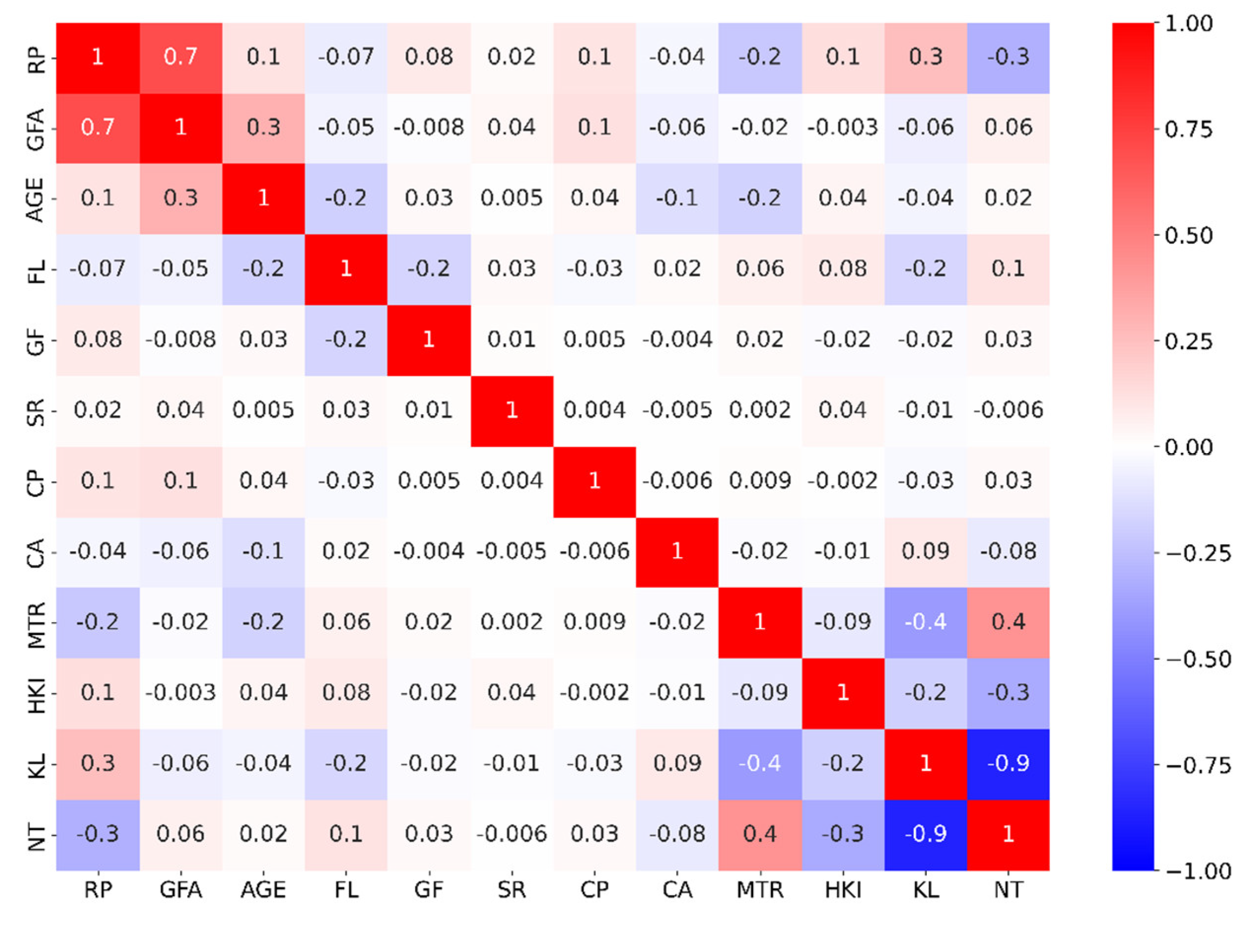
Figure 2 illustrates a correlation matrix, revealing the linear relationships between all features in the dataset. Our analysis uncovers a strong positive correlation (
r = 0.7) between footage area and property prices. Additionally, moderate correlations are observed between property prices and the following variables: NT (New Territories) location (
r = 0.3), and age, car park availability (CP), and Hong Kong Island (HKI) location (each with
r = 0.1).
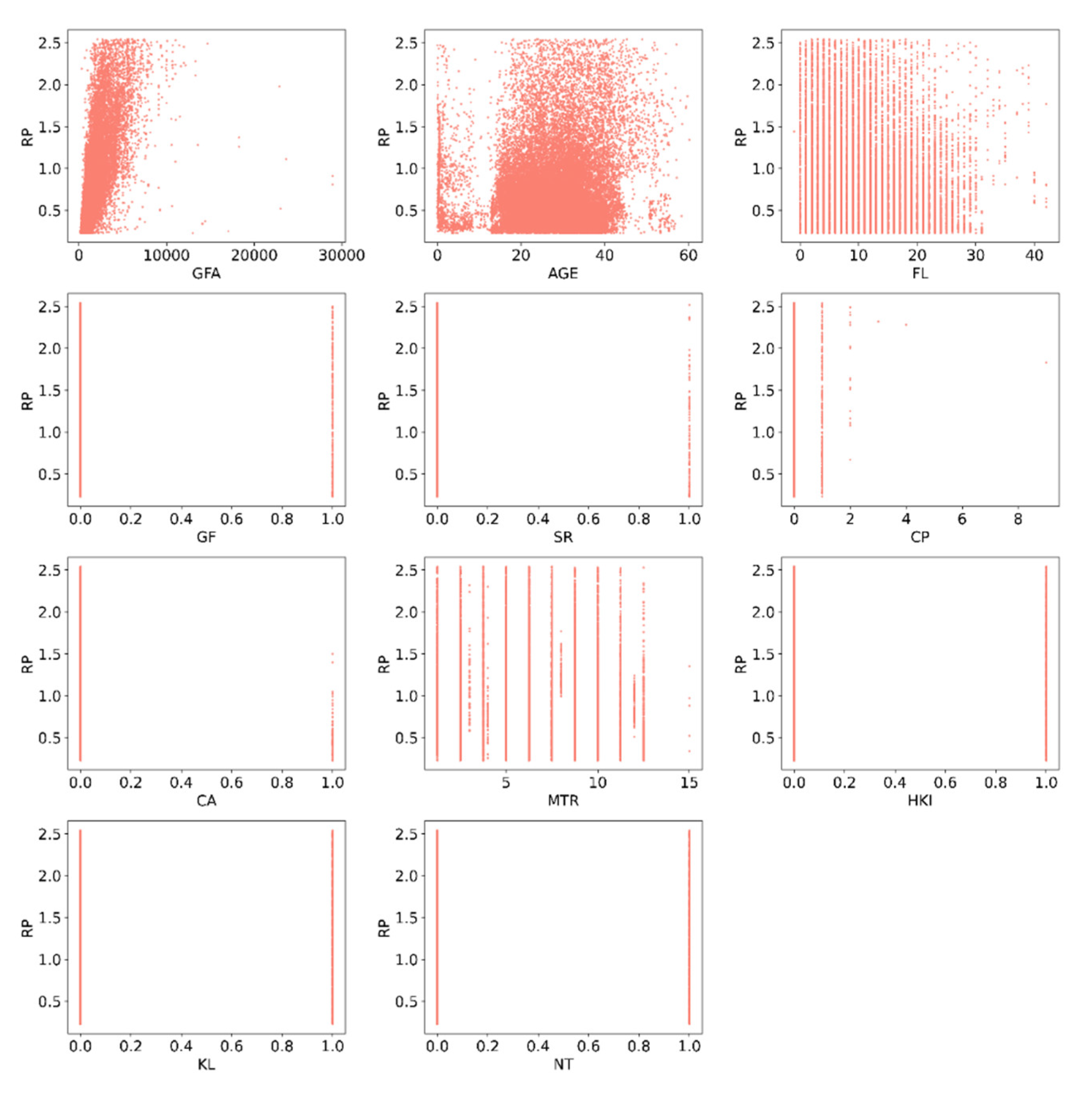
Figure 3 provides a visual representation of the data presented in
Figure 2, graphically illustrating the correlations between property prices and each explanatory variable. This visualization enhances the interpretability of the relationships identified in the correlation matrix.
Table 1 presents a summary of descriptive statistics for the variables employed in this study. These statistics offer a concise overview of the dataset’s central tendencies, dispersions, and distributions, either representing the entire population or a sample thereof. This exploratory analysis serves as a fundamental basis for subsequent statistical modeling and hypothesis testing, ensuring that the chosen analytical approaches are appropriate and aligned with the underlying data characteristics.
Results and Discussions
In our study, we employ a robust cross–validation technique to assess the performance and generalizability of our machine learning models. Specifically, we implement a 5–fold cross–validation approach, partitioning our dataset into five equal subsets or “folds.” The k–fold cross–validation method is applied as follows: in each iteration, four of the five folds (constituting 80% of the total sample) are utilized as the training set, while the remaining fold (20% of the sample) serves as the test set for generating predictions. This process is repeated five times, with each fold serving once as the test set.
This methodological approach offers several advantages. It enables a comprehensive evaluation of model performance across various subsamples of the data. Furthermore, it results in the development of five distinct models, each trained on a different subset of the data. Additionally, it allows for the assessment of each model’s predictive capability on previously unseen data. By employing this cross–validation strategy, we aim to mitigate overfitting and obtain a more reliable estimate of our models’ performance and generalizability. This approach is particularly valuable in scenarios where the available data is limited, as it maximizes the utility of the dataset for both training and evaluation purposes.
The optimization of hyperparameters for the GBM model is conducted through an extensive iterative process utilizing five–fold cross–validation.
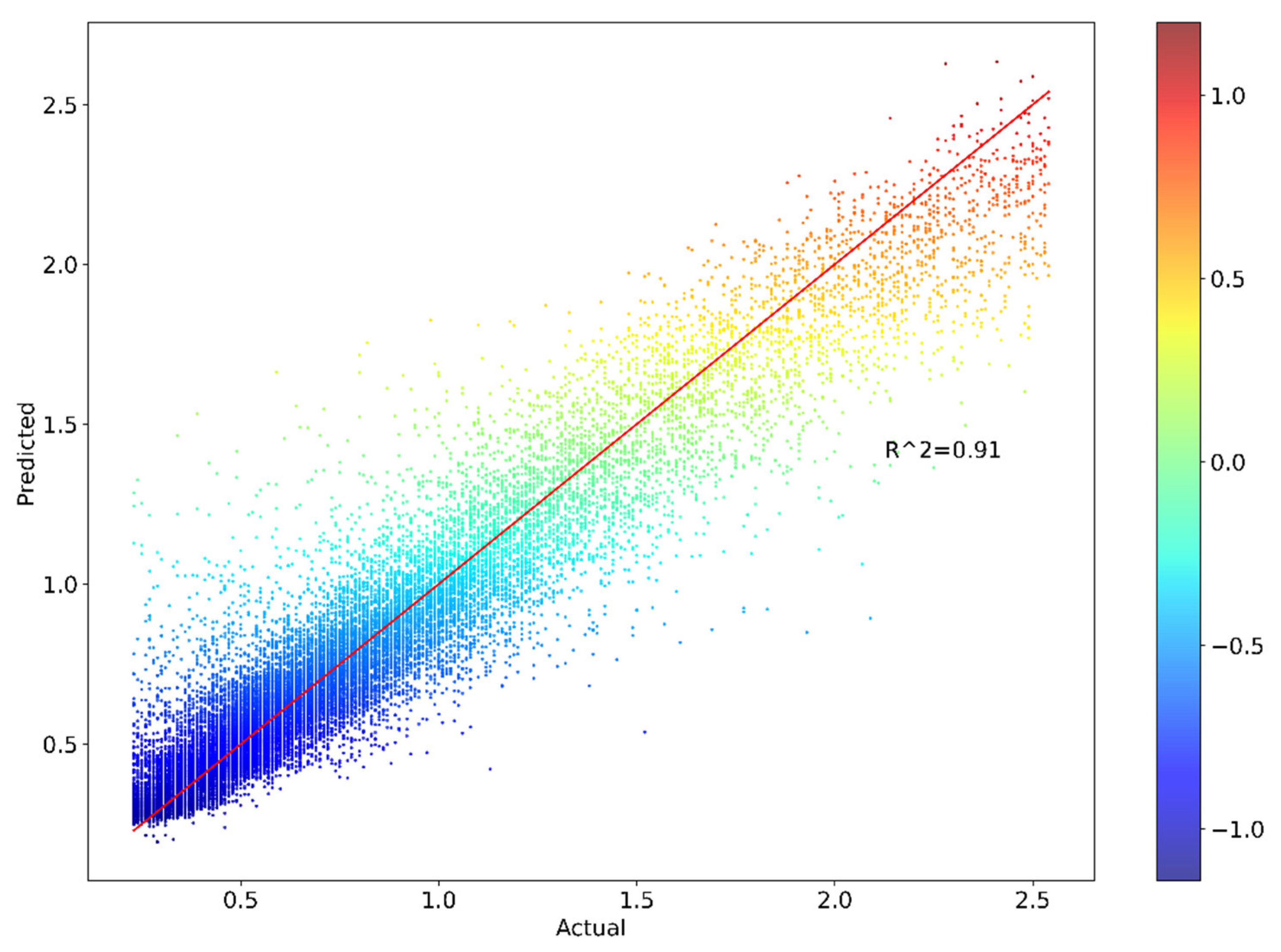
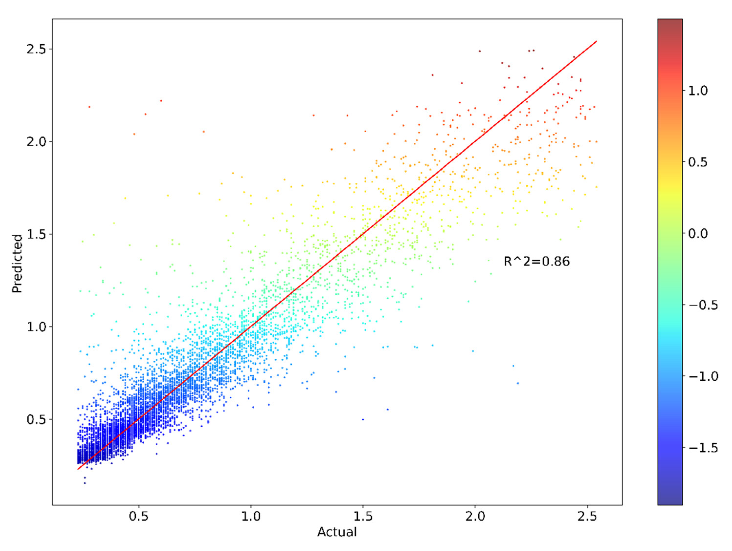
Table 2 delineates the hyperparameter space explored and the optimal values identified for various GBM parameters. The hyperparameters subject to fine–tuning included, but are not limited to, n_estimators, min_samples_split, min_sample_leaf, max_features, and max_depth. The optimization procedure involved multiple iterations of the entire five–fold cross–validation process, with each iteration employing distinct model configurations. This comprehensive approach allowed for a thorough exploration of the hyperparameter space. Subsequently, a comparative analysis of all resultant models is performed to identify the most efficacious configuration. The optimization process is facilitated by Optuna, a hyperparameter optimization framework. This methodology yields impressive results, with the optimal model achieving a coefficient of determination (
R²) of 0.90994 for the training set and 0.85724 for the test set. These high
R² values indicate a strong goodness of fit and predictive capability of the model.
Further evaluation of the model’s performance is conducted using multiple metrics. For the training set, the Mean Absolute Error (MAE) is 0.09041, the Mean Squared Error (MSE) is 0.01879, the Mean Absolute Percentage Error (MAPE) is 14.46240%, and the Root Mean Squared Error (RMSE) is 0.13708. The test set exhibited similar performance, with the MAE of 0.10704, MSE of 0.03051, MAPE of 16.49385%, and RMSE of 0.17467. The proximity of these evaluation metrics between the training and test sets is noteworthy. The marginal differences observed suggest that the model exhibits good generalization capabilities, effectively balancing bias and variance. This balance is crucial in machine learning models, as it mitigates the risks of overfitting or underfitting.
The absence of significant discrepancies between the training and test set evaluation metrics provides strong evidence that the model has not experienced overfitting, where a model performs exceptionally well on training data but fails to generalize to unseen data. Simultaneously, the high R² values and relatively low error metrics for both sets indicate that underfitting, where a model fails to capture the underlying patterns in the data, is also not a concern. In conclusion, the hyperparameter optimization process, coupled with rigorous cross–validation and comprehensive performance evaluation, has resulted in a robust GBM model that demonstrates excellent predictive capabilities while maintaining good generalization performance across both training and test datasets.
Figure 5 and
Figure 6 present the scatterplots of actual and predicted values of industrial property prices for both the training and testing datasets, respectively. In both plots, the actual and predicted values exhibit a strong correlation, with the majority of data points falling closely along the red line, indicating a good fit between the model’s predictions and the actual values. However, it is notable that there are some scattered points (whose actual values fall within the range of 1.5 to 2.2) that deviate significantly from the clustering of the majority of the data points. The strong correlation between the actual and predicted values suggests that the model has successfully captured the underlying patterns in the data, resulting in accurate predictions. The slight deviations from the clustering observed in some cases may be attributed to noise in the data or other factors that are not captured by the model.
The concluding phase of our analytical approach involves the application of SHAP values analysis to elucidate the predictive capabilities of industrial property prices. This analysis examines the relative importance of individual features and their influence on the model’s decision–making process, thereby providing profound insights into the factors driving real estate prices. To accomplish this, we employ the TreeExplainer module within the SHAP framework to interpret the predictions of the GBM model by calculating SHAP values for the test dataset. These SHAP values serve as measures of feature importance, quantifying the positive or negative contribution of each feature to each individual prediction, thereby illustrating the impact of each feature on the model’s predictions.
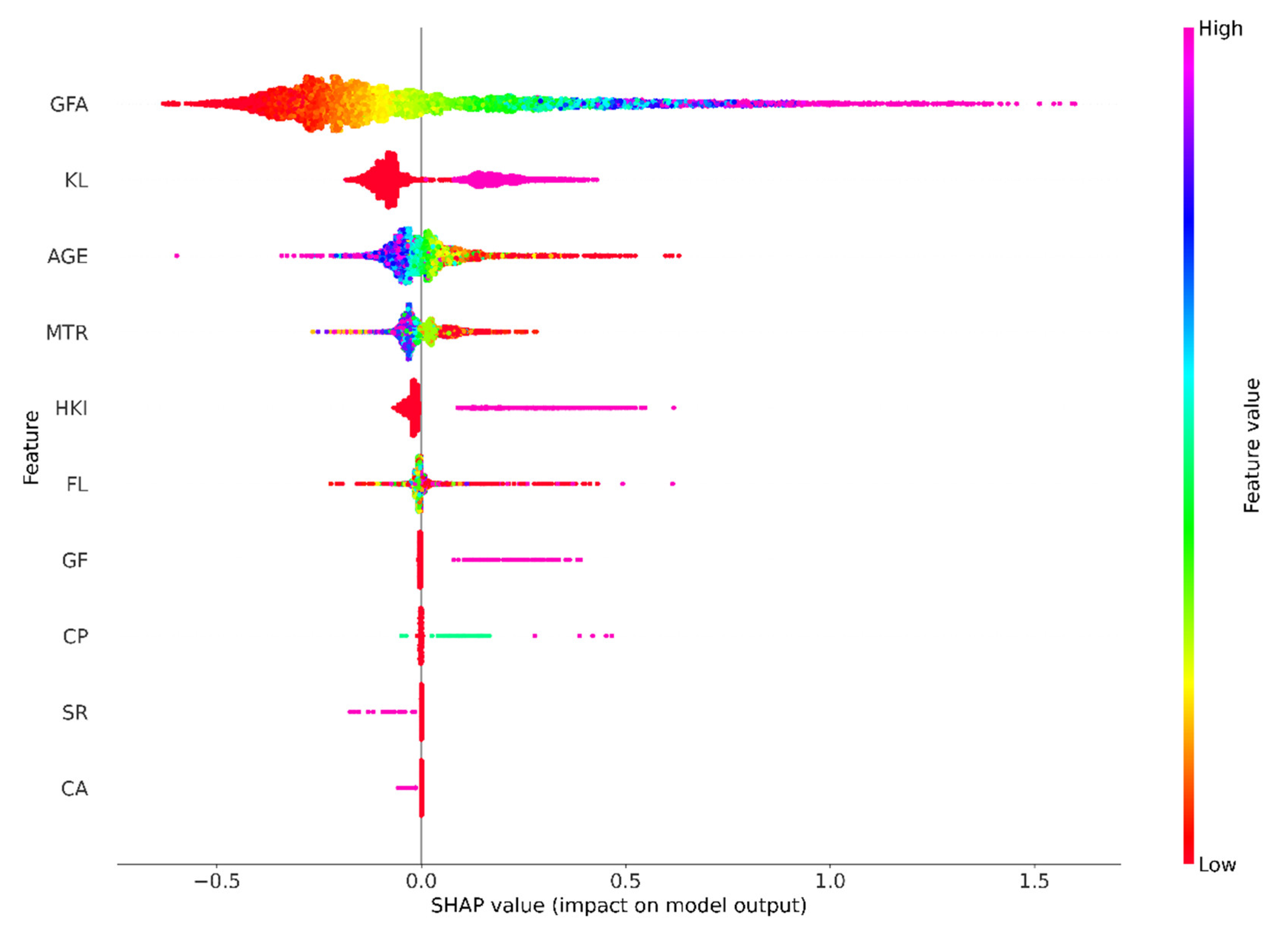
Figure 7 and
Figure 8 complementarily present the SHAP (SHapley Additive exPlanations) value analysis of the impact of features on the prediction of industrial property prices. These plots provide valuable insights into the most influential features for the model’s predictions and their effect on industrial property prices.
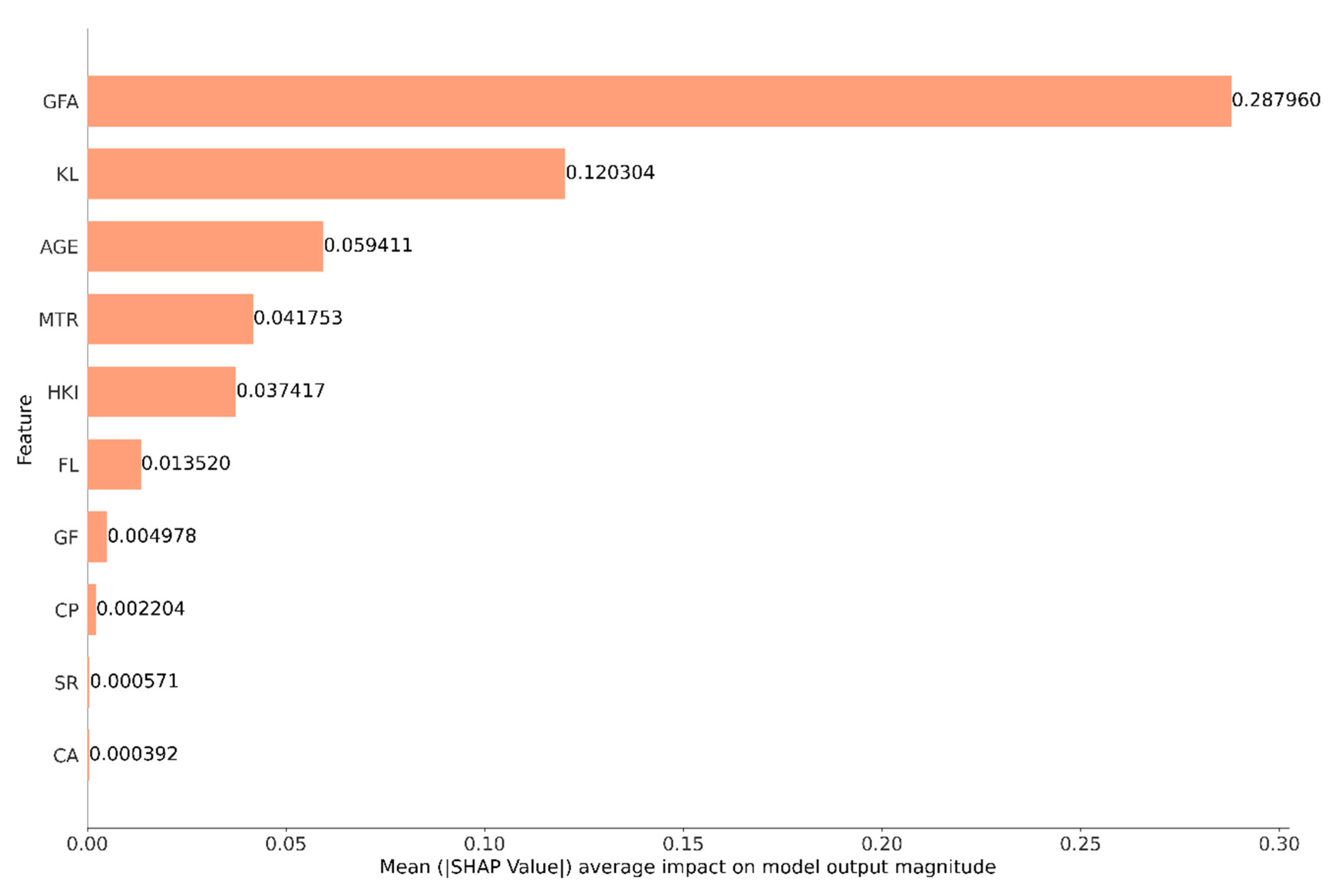
Figure 7 depicts the SHAP summary plot, which presents a summary of the mean absolute SHAP values for each feature, which serves as an indicator of its overall significance in influencing the model’s predictions. The features are ranked according to their importance, with the length of the bar representing the mean absolute SHAP value for each feature, thereby indicating its significance. A higher value indicates a more substantial impact on the predicted outcomes while the color–coded bars display the mean absolute SHAP values for each feature. Unlike traditional feature importances, mean absolute SHAP values are more straightforward and intuitive, as they are presented in the same units as the target variable, specifically HK
$ millions in our study. The analysis reveals that Gross Floor Area (GFA) is the most significant feature for the test set, with a SHAP value of 0.287960. A SHAP value of 0.287960 suggests that the GFA contributes approximately HK
$287,960 to the predicted property prices for a given observation, inflation–adjusted. In contrast, common area (CA) is the least informative feature, contributing only HK
$392 to each price prediction in the test set, inflation–adjusted.
Figure 8 presents the SHAP Summary plot (beeswarm), which visualizes the impact of each feature on the model’s prediction for individual instances. Each point represents a SHAP value for a feature and an instance, with high feature values colored magenta and low values colored red. The features are ordered according to the sum of SHAP magnitudes across all samples.
Figure 8 is used to illustrate the distribution of SHAP values for each feature across all data points. The x–axis position represents the impact of each feature on the model’s output, with features that increase predictions located on the right and those that decrease predictions situated on the left. The color intensity of the points corresponds to the feature’s value, with magenta indicating higher values and red indicating lower values. The distribution of points demonstrates the variability in the impact of each feature across different data points.
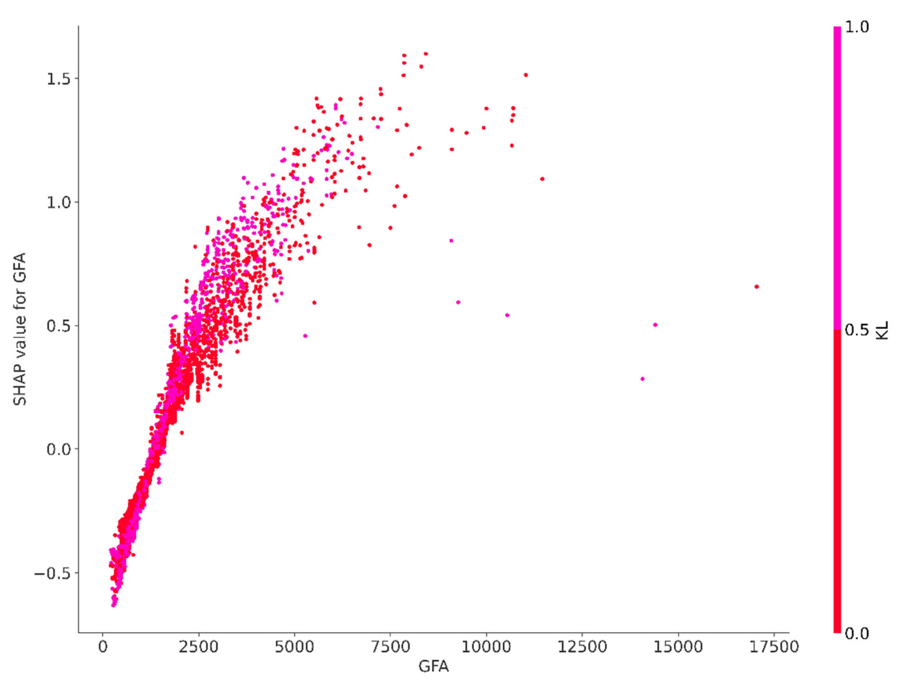
The results of the SHAP analysis reveal that gross floor area (GFA) significantly influences property prices, exhibiting the highest average impact among the features examined. This finding emphasizes the pivotal role that the size of industrial property plays in the determination of its price. The analysis further uncovers the presence of non–linear relationships, as evidenced by the wide distribution of GFA’s SHAP values illustrated in the beeswarm plot, which extends across both sides of the baseline. This suggests a complex interaction between GFA and price. While it is well established that larger properties typically command higher prices—a trend that is intuitively recognized in the real estate market—the variability in SHAP values indicates that this relationship is not universally linear. Smaller properties can also achieve elevated prices depending on various additional factors. Conversely, a larger area does not automatically guarantee a corresponding premium in price. The observable variability along the x–axis of the beeswarm plot suggests that the influence of GFA on price is subject to considerable inconsistencies. This pattern indicates the presence of non–linear dynamics wherein the effect of GFA on price does not consistently correspond with the property’s size. In some cases, an increase in GFA may result in a proportionate rise in price predictions; however, in other instances, the impact may be less pronounced or even inversely related. Such variability likely reflects the influence of market trends, property location, and the desirability of specific attributes.
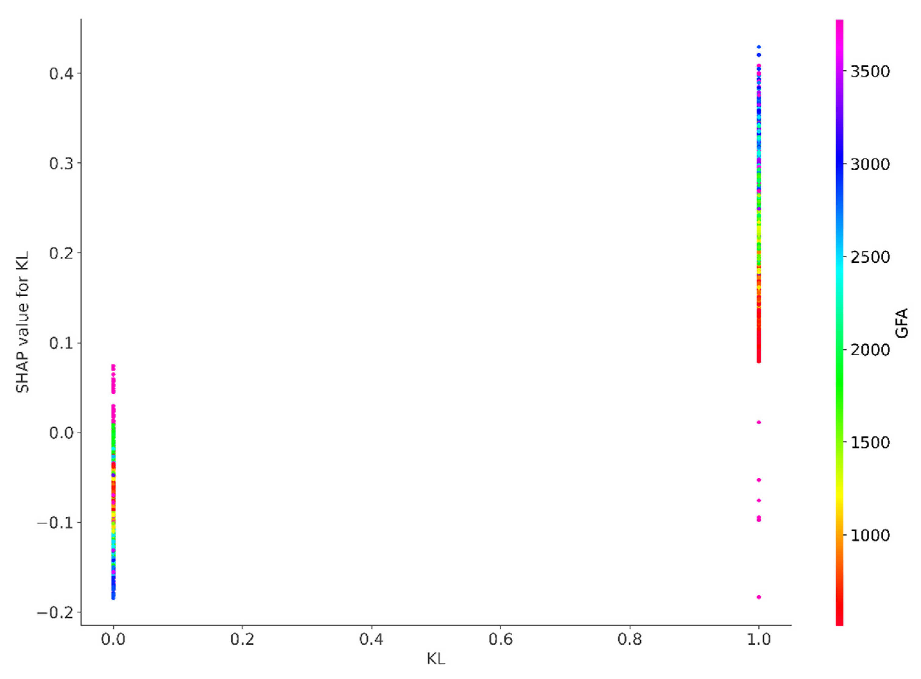
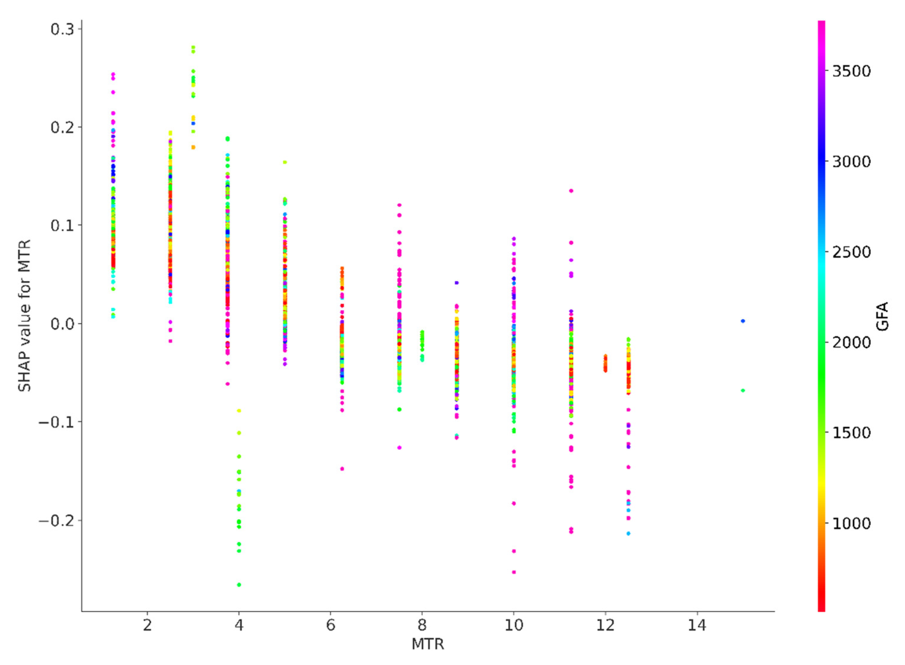
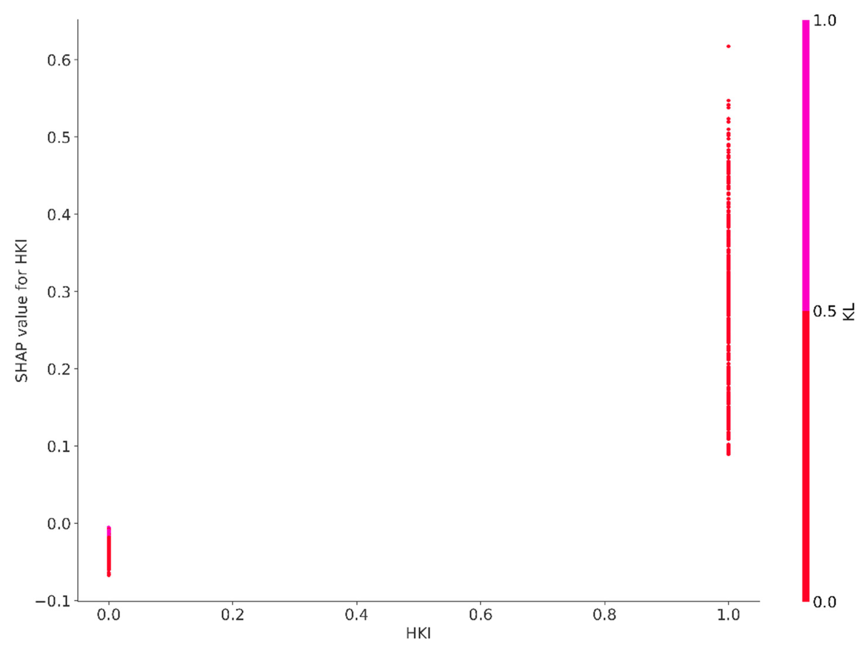
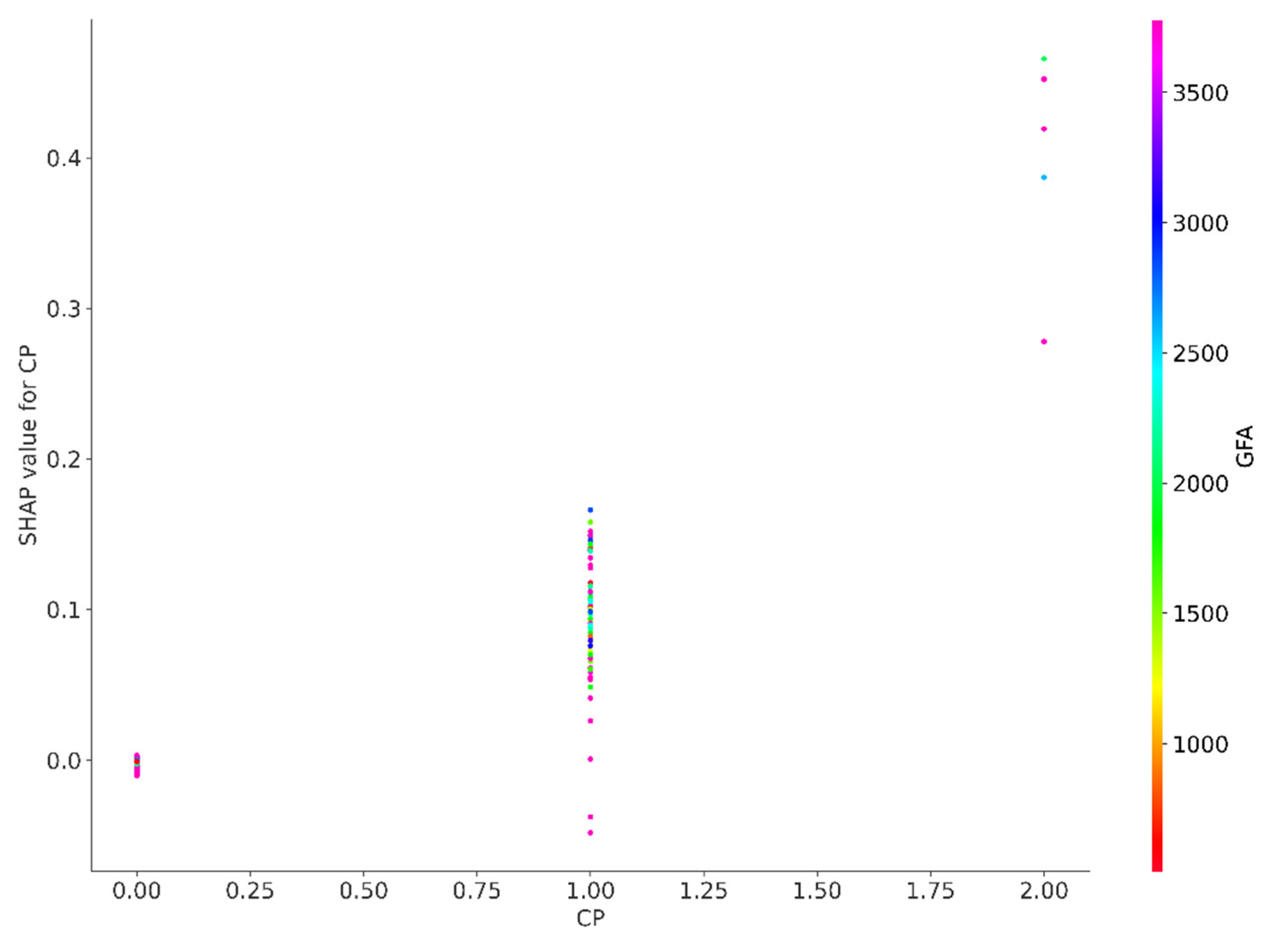
The SHAP values for the features Kowloon (KL), property age (AGE), accessibility to MTR (MTR), Hong Kong Island (HKI) floor level (FL) and car park (CP), as depicted in the beeswarm plot, similarly extend across both sides of the baseline. This distribution suggests the existence of non–linear dynamics, indicating that the effects of these features on property prices do not consistently correlate with their values. In certain instances, an increase in these features may lead to a proportionate rise in price predictions; however, in other cases, the impact can be less pronounced or even inversely related. Such variability likely reflects the influence of market trends, the geographical location of properties, and the desirability of specific attributes.
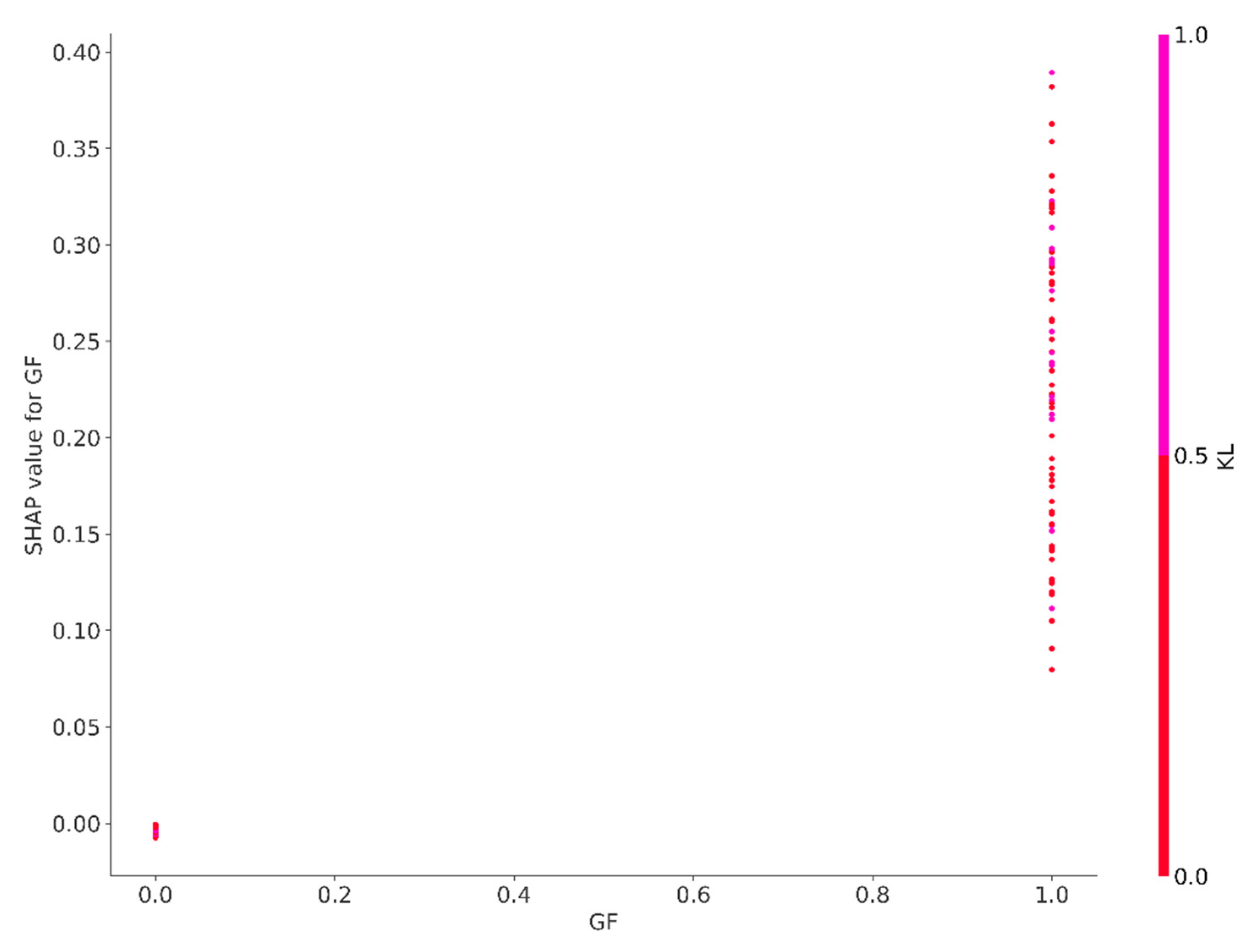
The SHAP value for the ground floor consistently appears on the right–hand side of the baseline, indicating a stable and positive influence of this feature on property prices. This consistent distribution suggests that industrial properties situated on the ground floor tend to command a price premium, highlighting the perceived value associated with this particular attribute. The favourable pricing of ground–floor locations may be attributable to several factors, including enhanced accessibility, increased visibility, and convenience for potential tenants or buyers, all of which contribute to the desirability of such properties in the industrial sector.
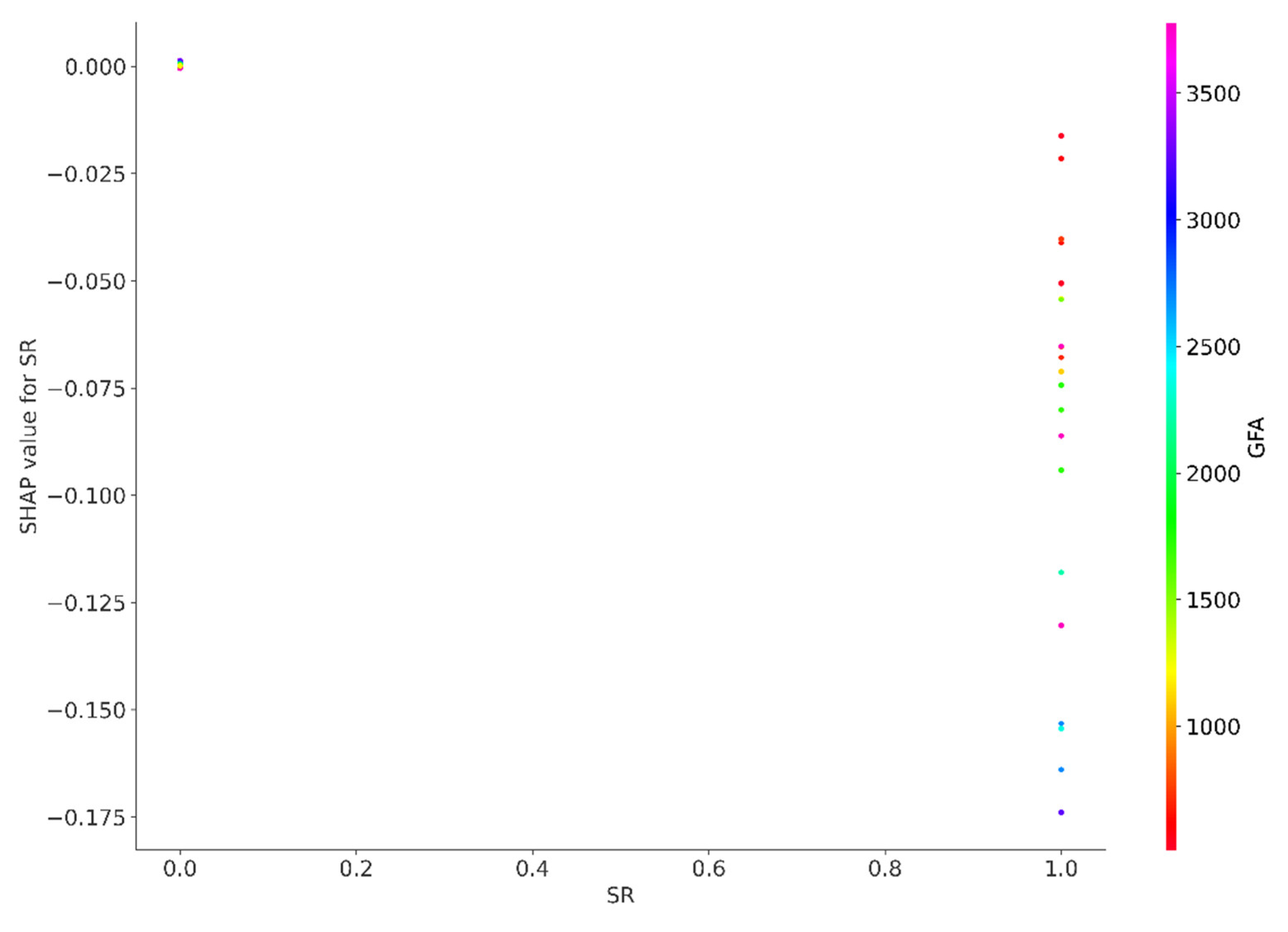
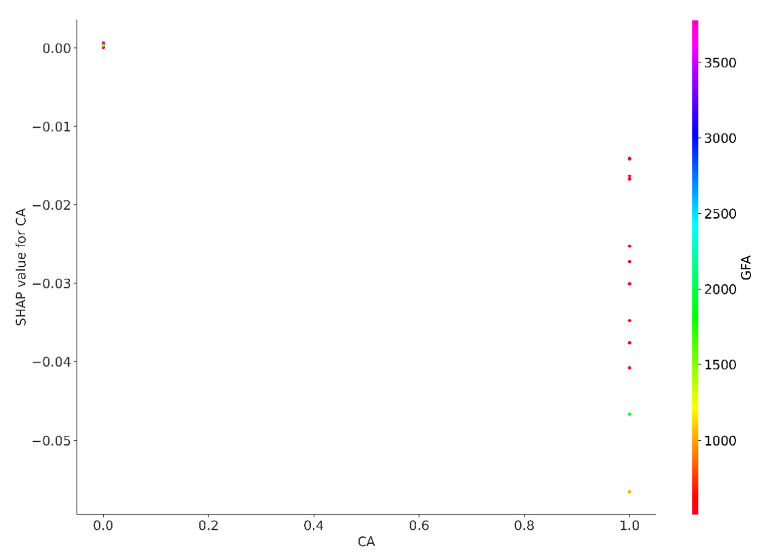
In contrast, the SHAP values for features such as store room (SR) and common area (CA) are consistently found on the left–hand side of the baseline. This placement implies that industrial properties incorporating a store room or a common area are likely to experience a reduction in their price, suggesting that these attributes may be viewed less favourably in the context of property valuation. The presence of these features could indicate a compromise on space efficiency or could detract from the market appeal of the property, leading to price concessions. This disparity in SHAP values between ground floor locations and the presence of store rooms or common areas underscores the complexity of buyer preferences and market dynamics that influence property pricing in the industrial real estate sector.
Conclusions
In conclusion, this study has employed machine learning techniques to investigate the dynamics of the industrial property market, a sector characterized by atypical market behavior. The results demonstrate that the utilization of SHapley Additive exPlanations (SHAP) provides transparency to the model’s decision–making processes, enabling the identification of critical predictors of real estate values. Specifically, proprietary data regarding property size and precise location emerge as significant factors, while open data variables related to accessibility to mass transit railway stations captures the contextual nuances of a property’s environment.
The practical implications of these findings are far–reaching for urban planners and policymakers. The integration of diverse data sources can refine urban development strategies by ensuring they are grounded in a comprehensive understanding of the factors influencing real estate values. This approach supports informed decision–making that promotes sustainable and equitable growth, enabling more targeted and effective urban planning policies that address the evolving needs and trends of the real estate market.
Furthermore, this study underscores the importance of transparency in AI–driven analytics. The use of tools such as SHAP heatmaps enhances model accountability and serves as a bridge for communication with non–technical stakeholders, rendering complex AI assessments more accessible and comprehensible. As the use of machine learning algorithms becomes increasingly prevalent in urban planning and policy–making, it is essential to prioritize transparency and accountability to ensure that these tools are used in a responsible and ethical manner.
This research contributes to the growing body of literature on real estate and urban economics by shedding light on the complexities of the industrial property market. The findings have significant implications for policymakers, developers, and other stakeholders seeking to understand the dynamics of this market. Future research could build upon this study by exploring other machine learning techniques and their applications in urban planning and policy–making.
Appendix A. SHAP Dependency Plots
This appendix presents a series of SHAP dependency plots intended to clarify the relationships between specific features and the model’s outputs. Each plot illustrates the variation in SHAP values, which reflect the contribution of individual features to the overall prediction, as the values of these features fluctuate. The visualizations presented in this section are essential for understanding the model’s behavior and the role of distinct features in influencing its predictions.
Figure A1.
SHAP value for GFA.
Figure A1.
SHAP value for GFA.
Figure A2.
SHAP value for KL.
Figure A2.
SHAP value for KL.
Figure A3.
SHAP value for MTR.
Figure A3.
SHAP value for MTR.
Figure A4.
SHAP value for HKI.
Figure A4.
SHAP value for HKI.
Figure A5.
SHAP value for FL.
Figure A5.
SHAP value for FL.
Figure A6.
SHAP value for GF.
Figure A6.
SHAP value for GF.
Figure A7.
SHAP value for CP.
Figure A7.
SHAP value for CP.
Figure A8.
SHAP value for SR.
Figure A8.
SHAP value for SR.
Figure A9.
SHAP value for CA.
Figure A9.
SHAP value for CA.
References
- Adams. D. (1990). “Meeting the needs of industry? The performance of industrial land and property markets in inner Manchester and Salford,” in Land and Property Development in a Changing Context Eds P Healey, R Nabarro (Aldershot, Hants: Gower) pp 113–127.
- Almaslukh, B. (2020). A gradient boosting method for effective prediction of housing prices in complex real estate systems. 2020 International Conference on Technologies and Applications of Artificial Intelligence (TAAI), Taipei, Taiwan, 2020, pp. 217–222. [CrossRef]
- Chau, K.W.; Chan, A.S.W. The determinants of industrial property prices during period of economic restructuring–The case of Hong Kong. Paper presented at the 14th Pacific Rim Real Estate Society Conference, Kuala Lumpur, Malaysia; 2008. [Google Scholar]
- Census and Statistics Department, 2013, Quick link of statistical products, Hong Kong SAR Government. Available online: http://www.censtatd.gov.hk/hkstat/srh/index.jsp?productTypeId=8&subjectCode=50.
- Census and Statistics Department. Table 210–06308: Employed persons by industry and occupation of main employment. 2024. Available online: https://www.censtatd.gov.hk/en/web_table.html?id=210-06308#.
- Daniels, P.W.; Bryson, J.R. Manufacturing services and servicing manufacturing: knowledge–based cities and changing forms of production. Urban Studies 2002, 39, 977–991. [Google Scholar] [CrossRef]
- Deppner, J. von Ahlefeldt–Dehn, B., Beracha, E.; et al. (2023). Boosting the accuracy of commercial real estate appraisals: an interpretable machine learning approach. Journal of Real Estate Finance and Economics. [CrossRef]
- Development Bureau. (2010) Optimizing the Use of Industrial Buildings to Meet Hong Kong’s Changing Economic and Social Needs. Hong Kong SAR Government. Available online: http://www.devb.gov.hk/industrialbuildings/eng/home/index.html.
- Frieman, J.H. Greedy function approximation: a gradient boosting machine. Annals of Statistics 2001, 29, 1189–1232. [Google Scholar]
- Hong Kong SAR Government, (2023), Hong Kong: The Facts – Trade and Industry. Available online: https://www.gov.hk/en/about/abouthk/factsheets/docs/trade_industry.pdf.
- Hong Kong SAR Government, (2024), Hong Kong – the Facts. Available online: https://www.gov.hk/en/about/abouthk/facts.htm.
- Kee, T.; Chau, K.W. Adaptive reuse of heritage architecture and its external effects on sustainable built environment—Hedonic pricing model and case studies in Hong Kong. Sustainable Development 2020, 28, 1597–1608. [Google Scholar] [CrossRef]
- Kee, T., Chung, T., Lee, H.Y. & Ho, P.P. Sustainable Revitalization – Adaptive Reuse of Industrial Buildings: 活現築蹟 -- 工廈 活化 新生. Commercial Press of Hong Kong 2019, 276 p. 2019.
- Kee, T. & Ho, Winky, K.O. Optimizing machine learning models for urban sciences: a comparative analysis of hyperparameter tuning methods. Preprints 2024, 2024060264. [Google Scholar] [CrossRef]
- Lenaers, I. & de Moor, L. Exploring XAI techniques for enhancing model transparency and interpretability in real estate rent prediction: A comparative study. Finance Research Letters 2023, 58, 104306. [Google Scholar] [CrossRef]
- Lorenz, F. Willwersch, J., Cajias, M., & Fuerst, F. Interpretable machine learning for real estate market analysis. Real Estate Economics 2023, 51, 1178–1208. [Google Scholar] [CrossRef]
- Lundberg, S.M. & Lee, S. I. A unified approach to interpreting model predictions. Paper presented at 31st Conference on Neural Information Processing Systems (NIPS USA, 2017.
- Lundberg, S.M. Erion, G., Chen, H., DeGrave, A., Prutkin, J.M., Nair, B., Katz, R., Himmelfarb, J., Bansal, N. & Lee , S.I. From local explanations to global understanding with explainable AI for trees. Nature Machine Intelligence 2020, 2, 56–57. [Google Scholar] [CrossRef] [PubMed]
- Lundberg , S.M. Nair, B., Vavilala, M.S., Horibe, M., Eisses, M.J., Adams, T., Liston, D.E., Low, D.K.W., Newman, S.F., Kim, J. & Lee, S.I. Explainable machine learning predictions for the prevention of hypoxaemia during surgery. Nature Biomedical Engineering 2018, 2, 749–760. [Google Scholar] [PubMed]
- Neves, F.T. Aparicio, M. & Neto, M. de Castro The impacts of open data and eXplainable AI on real estate price predictions in smart cities. Applied Sciences 2024, 14, 2209. [Google Scholar] [CrossRef]
- Rating and Valuation Department (2024). In Hong Kong Property Review; Hong Kong SAR Government.
- SHAP, (2018). Welcome to the SHAP documentation. Available online: https://shap.readthedocs.io/en/latest/.
- Shapley, L.S. A value for n–person games. Contributions to the Theory of Games 1953, 2, 307–317. [Google Scholar]
- Sharma, S. Arora, D., Shankar, G., Sharma, P. & Motwani, V. (2023). House price prediction using machine learning algorithm. 2023 7th International Conference on Computing Methodologies and Communication (ICCMC), Erode, India; 2023; p. 982. [Google Scholar] [CrossRef]
- Sit, V.F.S. Industrial transformation of Hong Kong, in The Hong Kong–Guangdong Link: Partnership in Flux Eds, R Y W Kwok, A Y So (Hong Kong University Press, Hong Kong) pp. 163–186. 1995. [Google Scholar]
- Swathi, B. & Shravani, V. House price prediction analysis using machine learning. International Journal for Research in Applied Science & Engineering Technology 2019, 7, 1483–1492. [Google Scholar]
- Tang, B.S. & Ho, Winky, K.O. Cross–sectoral influence, planning policy and industrial property market in a high–density city: A Hong Kong study 1978 – 2012. Environment and Planning A: Economy and Space 2014, 46, 2915–31. [Google Scholar]
- Tang, B.S. & Ho, Winky, K.O. Land–use planning and property market adjustment: restructuring of industrial space in Hong Kong. Land Use Policy 2015, 43, 28–36. [Google Scholar]
- Wood, B. & Williams, R. (Eds), 1992, Industrial Property Markets in Western Europe (E& FN Spon, London).
- Yeh, A.G.O. Economic restructuring and land use planning in Hong Kong. Land Use Policy 1997, 14, 1997, 25–39. [Google Scholar] [CrossRef]
- Yeh, A.G.O. and Ng, M. K. The changing role of the state in high–tech industrial development: The experience of Hong Kong, Environment and Planning C: Government and Policy 1994, 12, 449–472. [Google Scholar]
|
Disclaimer/Publisher’s Note: The statements, opinions and data contained in all publications are solely those of the individual author(s) and contributor(s) and not of MDPI and/or the editor(s). MDPI and/or the editor(s) disclaim responsibility for any injury to people or property resulting from any ideas, methods, instructions or products referred to in the content. |
© 2024 by the authors. Licensee MDPI, Basel, Switzerland. This article is an open access article distributed under the terms and conditions of the Creative Commons Attribution (CC BY) license (http://creativecommons.org/licenses/by/4.0/).
