Pan-Arctic Lead Maps based on Sentinel-1 SAR Images with a Convolutional Neural Network

The Sentinel-1 SAR Extra Wide swath mode with its 40 meters pixel size allows accurate lead mapping in Arctic sea ice areas. We present an improved winter lead detection algorithm based on a modified U-Net convolutional neural network. We introduce a preprocessing procedure that balances normalized radar cross section (NRCS) values between sub-swaths. This results in more consistent Sentinel-1 SAR images as input for the classifier, which is especially important for the cross-polarization HV channel. In turn, image consistency is essential for automatic image semantic segmentation. We develop a new lead detection algorithm and compare it with a previously published version. We produce pan-Arctic, 40 meters resolution lead maps and present pan-Arctic lead area fraction on a 12 km grid for January 2019. Within different Arctic regions, the lead area fraction is stable and varies only within the expected natural variability during the one month studied here. The average Arctic-wide lead area fraction is 2.44 % with 0.25 % standard deviation during January 2019. The improved lead detection algorithm leads to a better lead discrimination and extends the applicability area to the entire Arctic.

Keywords:

Subject: Environmental and Earth Sciences - Remote Sensing

1. Introduction

Sea ice covers a significant part of the Arctic Ocean. Its presence and harsh weather conditions make in-situ studies of the region difficult. As the Arctic is an important part of the Earth climate system, the knowledge of ice conditions in the Arctic is required for weather forecasting, climate, and ecosystem studies. In addition, sea ice information is important for shipping and offshore operations. Despite limitations, satellites are the only means to provide regular Arctic-wide information on the sea ice conditions. Due to the increase in the amount of satellite data, the development of algorithms for automatic data analysis is needed.

The presence of sea ice leads is one of the important features of the Arctic sea ice cover. They open due to sea ice dynamics forced by wind and ocean currents. For the winter-time pack ice in the Central Arctic they are the main reasons for the heat loss from the comparably warm ocean to the cold atmosphere. Here a large fraction of the thermodynamic sea ice growth takes place, and also ecological activity is observed in open cracks in sea ice cover.

Leads have been the subject of studies based on measurements from various satellite instruments. Lead fractions were derived from optical and thermal infrared images [1,2,3], passive microwave radiometer data [4], and altimeter measurements [5,6]. With the increased amount of Synthetic Aperture Radar (SAR) sensors in space, the Arctic Ocean now is covered by active microwave measurements at a high temporal resolution (daily to weekly coverage depending on the satellite constellation and the region) and SAR provide a better spatial resolution than other microwave satellite sensors, which is beneficial for lead detection. As a consequence, development of algorithms for automatic ice – open water discrimination for SAR images becomes more important. Methods proposed are based on backscatter thresholds [7,8], linear kinematic feature detection [9,10,11], and deviations in the SAR derived wind speed field [12]. For full polarimetric SAR scenes, a range of polarimetric features is introduced and used for surface type discrimination, including separation of ice and open water [13,14,15,16,17]. In case all four polarizations are not available, texture features based on gray level co-occurrence matrix are often used [18,19,20,21]. The use of the combination of polarimetric and texture features is studied in [22]. Most of these studies, however, were conducted only for a small set of SAR scenes.

In the last years convolutional neural networks (CNNs) are applied to satellite image analysis more and more often. A CNN for sea ice type classification on Sentinel-1 SAR images is described in [23]. CNNs are used for automatic sea ice chart production algorithms: [24] suggests the U-Net architecture for this task, and [25] uses a CNN architecture based on dilated convolution kernels. A lead detection method for Sentinel-1 images based on modified U-Net is suggested in [26], and another method with entropy-weighted network is introduced and compared with U-Net and DeepLabv3plus in [27].

In a preceding study, we have applied texture analysis techniques and a Random Forrest classifier for lead detection on Sentinel-1 SAR images [28]. In this paper, we build on that and introduce an improved classification algorithm based on U-Net [29] convolutional neural network that allows us to routinely apply the lead detection algorithm on all EW Sentinel-1 scenes taken over the Arctic. We compare results of the new algorithm with the previous algorithm based on traditional machine learning techniques, gray-level co-occurrence matrix features with Random Forest classification from [28]. With two satellites the Sentinel-1 constellation is able to cover almost the entire Arctic Ocean every three days with scenes taken in Extra Wide (EW) mode, and thus provide potential for large-scale lead monitoring and analysis. As the result, we are able to produce 3-day composite lead maps of the entire Arctic with the native 40 meter pixel size of the Sentinel-1 EW product. Despite a lower temporal coverage compared to passive microwave measurements which provide sea ice concentration maps daily (e.g., [30]), the Sentinel-1 based lead maps have unprecedentedly high resolution over the entire Arctic, independently of cloud and weather conditions.

2. Methods

2.1. Existing Lead Classification Method

In this section, we shortly explain the original algorithm discussed in [28] and then describe in details the improved lead detection algorithm presented in this study. The previously published method for the detection of leads is based on texture analysis of Sentinel-1 SAR images taken in the Extra Wide (EW) swath mode with 40 meters pixel size. The scenes downloaded from the Copernicus Open Access Hub (https://scihub.copernicus.eu) are calibrated to

γ_{0}

values with the calibration and noise look up tables provided in the metadata of the SAR datasets. Since sea ice backscatter depends on the incidence angle, an incidence angle correction with the coefficient 0.213 is applied to the HH channel. Then the polarization ratio HH / HV is calculated. Throughout the next steps of the classification the two images, (i) the HH channel and (ii) the polarization ratio, are considered separately. At the end, the final result of the classification is calculated as the combination of the two branches. Figure 1 shows an example of the individual lead classification steps and the final binary lead classification result.

In short, the existing lead classification from [28] consists of the following steps: The

5 \times 5

pixel bilateral filter is applied to images to reduce speckle noise [31]. After that, texture descriptors based on gray-level co-occurrence matrix (GLCM) are calculated for

9 \times 9

pixel windows surrounding every second pixel of the scene in each direction at 1-pixel distance [32]. As the result, the resolution of texture descriptors is two times coarser than the input Sentinel-1 scene. The window size is set to 9 pixels in order to collect enough statistics on texture on one side, and to be able to resolve leads of several pixel width on the other side. An increase of the window size would increase the minimal lead size that can be detected. On the other hand, a decrease of the window size would increase ambiguities in texture descriptors. In the next step, the texture descriptors are passed as input features to the Random Forest Classifier [33,34]. The classifier calculates probabilities for each pixel to represent a part of a lead based on the texture of the pixel surrounding. The resolution (pixel size) of the result is 80 meters. In the Murashkin et al. article [28], describing the first version of the lead detection algorithm, we suggested to use a threshold, e.g., 50%, for probabilities to produce a binary lead map.

Based on this previous work we here propose an improved Sentinel-1 lead detection algorithm. The first update to the algorithm is the improved Sentinel-1 EW preprocessing procedure that balances backscatter between sub-swath, i.e., brightness of the SAR image (Section 2.2). The second update is the use of a U-Net convolutional neural network instead of GLCM feature calculation and random forest classification (Section 2.3).

2.2. Improved Sentinel-1 Preprocessing

The previously suggested preprocessing algorithm used a scalloping noise correction (provided within the Sentinel-1 meta data since 13 March 2018). However, the backscatter corrected with the thermal noise vector provided with the default Sentinel-1 auxiliary data shows discrepancies at the sub-swath boundaries, especially pronounced on the cross-polarization channel, which has been addressed by [35,36,37]. To correct for the discrepancies, we apply a sub-swath balancing technique, that brings Normalized Radar Cross Section (NRCS) values within different sub-swath to a uniform scale. The thermal noise data provided in the Sentinel-1 auxiliary data show discrepancies at the sub-swath borders. We assume that the range dependence of thermal noise within a sub-swath has little discrepancy, whereas the absolute value has some error and can be corrected with a scale factor

α

n o i s e_{S W_{i}}^{c o r} \to α \cdot n o i s e_{S W_{i}}^{r a w}

(1)

S W_{i}

is the i-th sub-swath, cor is the corrected value, raw is the raw value.

n o i s e_{S W_{i}}^{c o r}

is the corrected noise value in the sub-swath

S W_{i}

n o i s e_{S W_{i}}^{r a w}

is the raw noise value in the sub-swath

S W_{i}

, provided as look-up tables in the auxiliary data. To ensure the land does not introduce a variation, significantly larger than that of sea ice, the maximal NRCS values are limited with 700 for the HH channel and 300 for the HV channel for the sub-swath balancing coefficient calculation. We assume Sentinel-1 scenes to be homogeneous at the sub-swath border, therefore, average NRCS values should not change drastically from one sub-swath to the next one. Thus, the SAR NRCS values averaged in along track direction should be continuous in the range direction.

D N_{S W_{i}}^{2} - n o i s e_{S W_{i}} = D N_{S W_{i + 1}}^{2} - α \cdot n o i s e_{S W_{i + 1}}

(2)

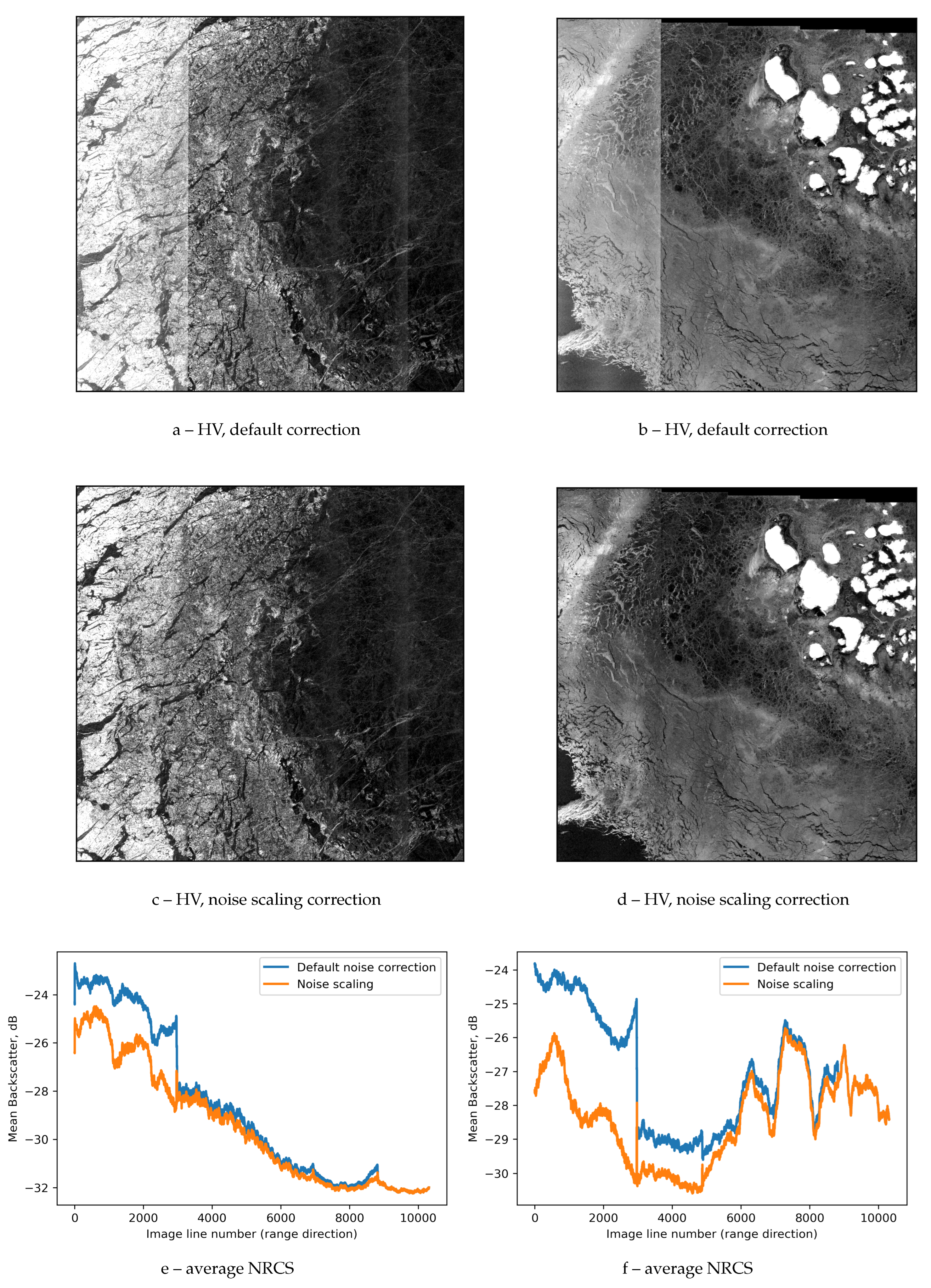
where

D N

is Digital Number (the value provided in the Sentinel-1 level 1 product before calibration) averaged in along track direction at the sub-swath

S W_{i}

to sub-swath

S W_{i + 1}

transition. The 5th sub-swath is taken as reference and its scale factor is 1, 1st to 4th swaths are brought to the NRCS values of the 5th sub-swath, see Figure 2e,f. Then, the noise scale factor can be calculated with

α = (D N_{S W_{i}}^{2} - D N_{S W_{i + 1}}^{2} + n o i s e_{S W_{i}}) / n o i s e_{S W_{i + 1}}

(3)

Scaling thermal noise for the adjacent sub-swath by

α

allows us to produce a more uniform Sentinel-1 image, which improves image classification robustness. An illustration of the preprocessed Sentinel-1 scenes is shown in Figure 2. Figure 2a,b show two Sentinel-1 EW HV channels with the preprocessing procedure suggested by ESA, with the noise tables provided as Sentinel-1 meta data, applied. The different sub-swaths are still noticeable, especially sub-swath 1 (left part of images). The same images with sub-swath balancing applied are shown in Figure 2c,d. Figure 2e,f show NRCS values averaged along the azimuth direction. The abrupt changes in average brightness between swaths with the basic noise correction applied (blue line) are eliminated with the swath balancing applied (orange line).

The preprocessing procedure is available online as a python library: https://github.com/d-murashkin/sentinel1_routines

2.3. Improved Lead Detection

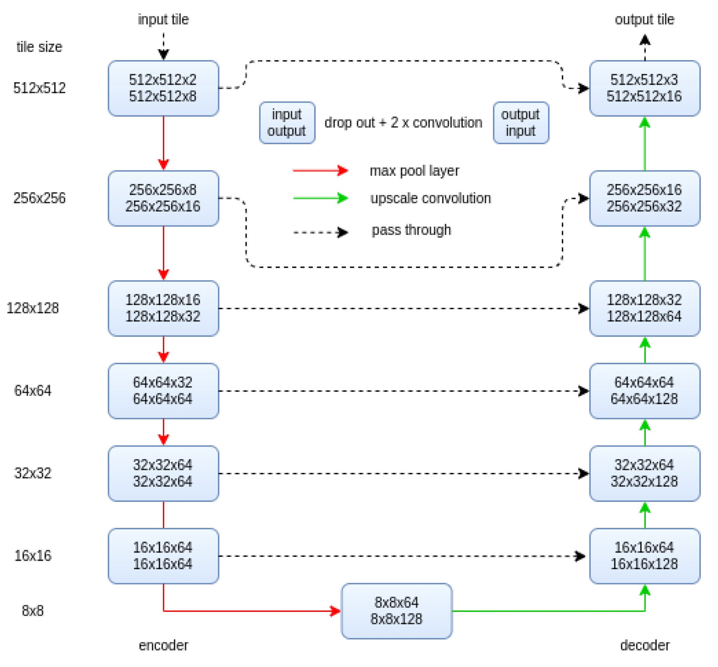
For lead detection, we use the U-Net convolutional neural network introduced in [29]. It is represented by a multi level encoder-decoder architecture, where encoder and decoder are connected on every level. We increased the depth of the encoder and the decoder to six layers compared to four layers suggested in the original study, the algorithm is schematically shown in Figure 3. This is done to increase the "field of view" of the convolution layers stack (or the "effective size of the convolution layers stack"). Further increase would require increase of the input tile size and increase of the computational complexity of the algorithm. A preprocessed Sentinel-1 image is split into 512-pixel square patches. The input for the model consists of a stack of the patches. Each of them has two channels: the HH channel and HV channel, and therefore the input has the dimension 512x512x2 pixels. Both channels are normalized to [-1; 1] with following values:

- 29

dB and 4 dB for the HH channel,

- 32

dB and

- 15

dB for the HV channel. Values below the minimal value and above the maximal value are cut out. This range of values covers the backscatter range for most sea ice types, except of maybe some ridges, which may have a higher backscatter values, however this should not affect the lead detection. These thresholds are used for all scenes to ensure the consistency of the normalized images. Every block of the diagram on the Figure 3 consists of a 50% dropout layer [38] followed with two convolutional layers with 3x3 convolution kernel size and ReLu activation function [39]. To retain the original image size, convolutional layers are applied with the padding same option. Red arrows represent max pool layer, which decreases the image size by a factor of two and keeps only the maximal value in every block of 2x2 pixels. Green arrows show upscale convolution layers, where image size in increased twice. The output layer includes

L_{2}

kernel regularization [40] and a softmax activation function and provides output class probabilities.

The training data annotations are converted to one hot labels, thus every pixel has a number for every label type representing weight of each label for the pixel. In order to balance the labels, one hot label values are weighted by the number of samples in the corresponding class. As the result, the input from each class to the loss function is the same, even in case the number of samples in each class differs. In addition to the three classes: “dark leads”, “bright leads”, and “sea ice”, we also introduce an extra, 4th class for unlabeled data. The one hot label value for the unlabeled data class is 0, therefore it has no influence on the loss value and therefore does not affect the training process. At the same time, it allows us to label irregular shape objects and provides a certain flexibility to the labeling process. On the one hand, not every pixel has to be labeled, on the other hand small leads can also be labeled even if they are smaller then the typical box size in case of box labeling.

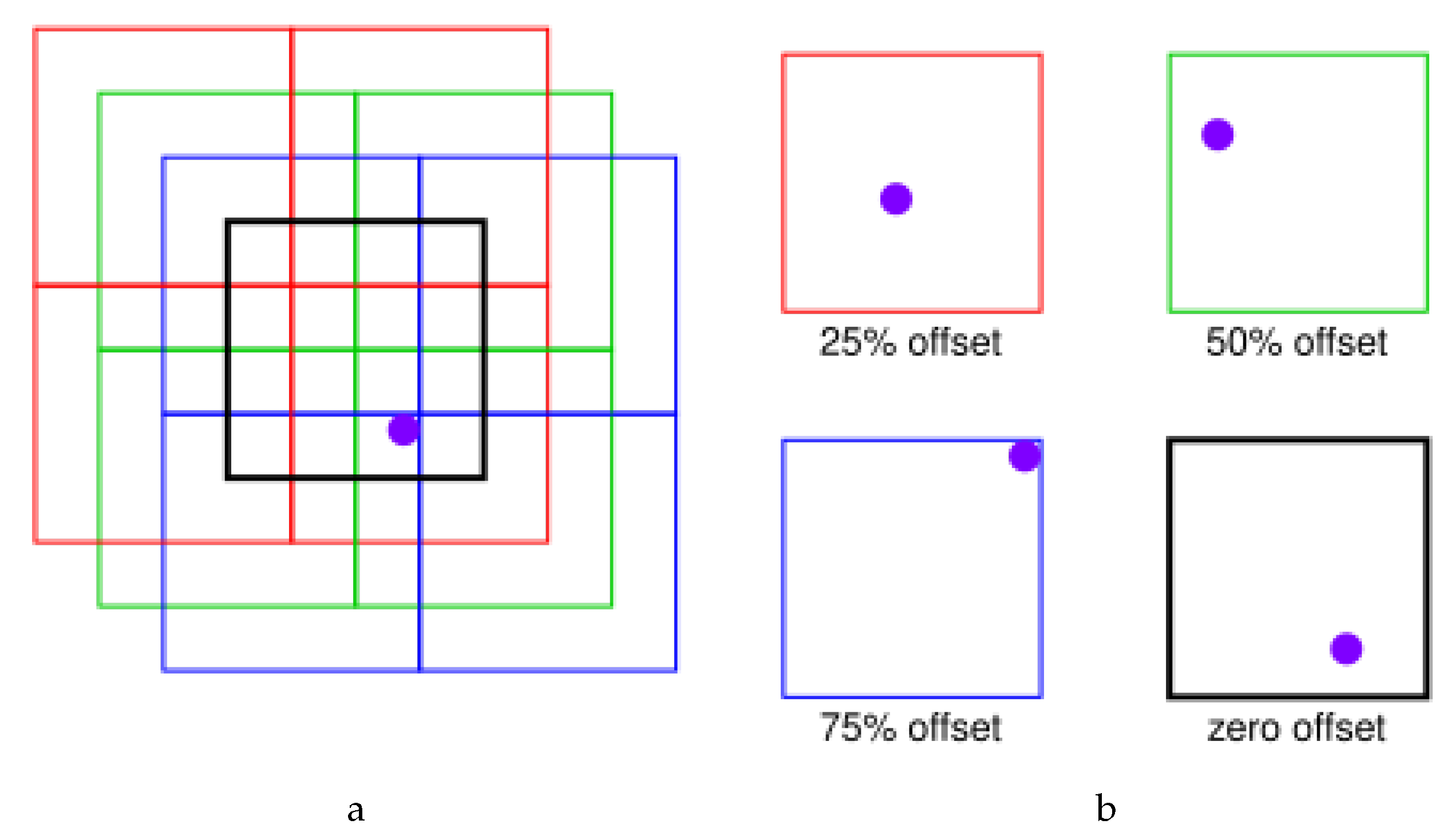
Splitting images into tiles leads to appearance of edge effects at patch edges on the corresponding classified image. This happens due to lack of context around pixels at, or close to, tile edges. To reduce this effect, we apply classification four times to every image. Each of the four times the Sentinel-1 preprocessed image is split into tiles with an offset as shown in Figure 4. Frames in black, red, green, and blue colors correspond to 0% (no offset), 25%, 50%, and 75% relative offset. Every pixel of a classified tile is weighted linearly between zero and one by its distance from an edge (weight 0) to the middle (weight 1) of the tile. This way, the classification result for a pixel in the middle of a tile has a higher weight compared to a pixel at an edge of the tile. Four weighted probabilities (one per offset) are summed up to the final classification result. For instance, a pixel shown in purple in the input scene in Figure 4 will appear at the middle of the red tile (split into tiles with 25% offset), closer to an edge of the green and black tiles (split into tiles with 50% and 75% offset), and at the edge of the blue tile (75% offset). Therefore, the lead probability, produced by the model applied to the red tile, has the highest contribution to the final result, while the lead probability, produced by the model applied to the blue tile, has the lowest contribution. The influence of near-border pixels on the per-pixel classification is, thus, decreased.

Output of the model consists of three channels with probabilities for the three surface classes: sea ice, dark lead, and bright lead. Dark leads are the leads appearing dark on the HH channel due to their smooth surface. These represent leads under calm open water conditions or refreezing leads with thin smooth layer of sea ice. Bright leads appear bright on the HH channel, but typically dark on the HV channel. These leads correspond to wind-roughened surface or thin sea ice with rough surface. The training data consists of 21 manually labeled Sentinel-1 images, collected over Fram Strait, Beaufort Sea, Barents Sea, and Kara Sea, with dark and bright leads marked with a different label. The training data is splits with 80% of the data set is used at train subset and 20% is used as test subsets.

3. Results

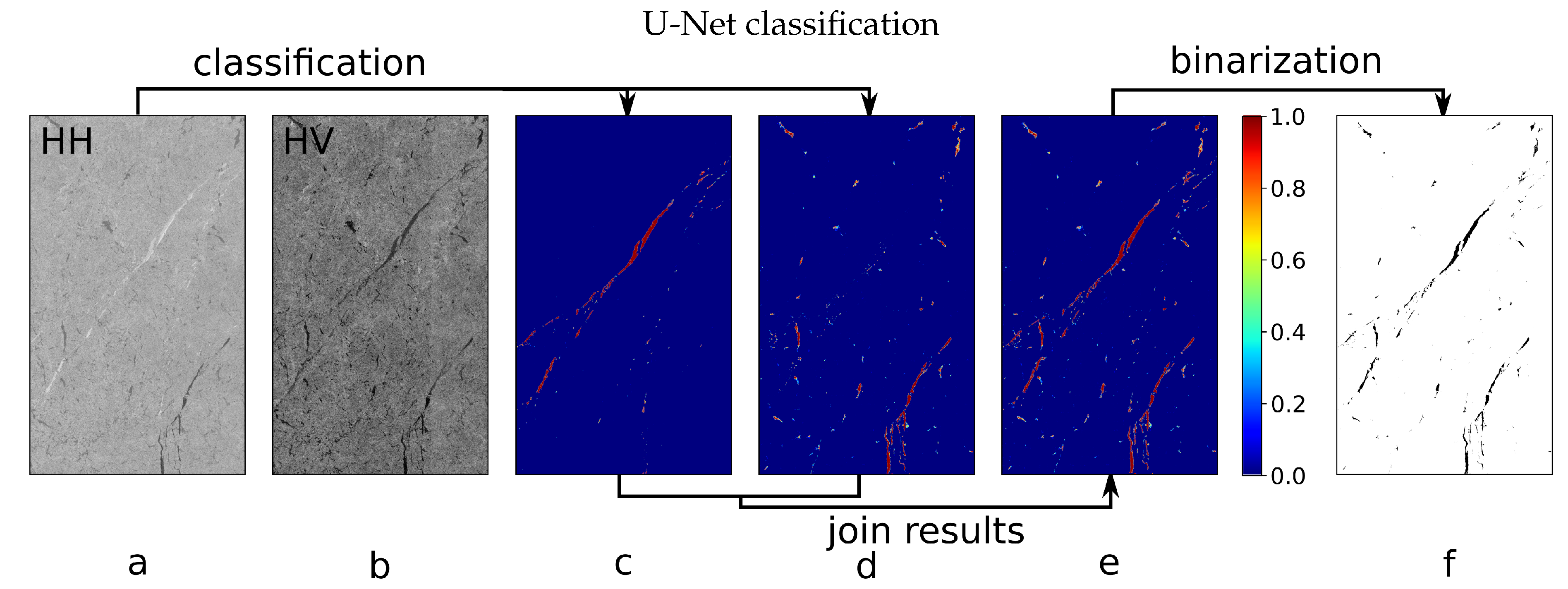
The U-Net -based classification workflow with results is shown in Figure 5. The HH (Figure 5a) and HV (Figure 5b) channels, preprocessed as described in Section 2.2, are passed to the U-Net -based classifier described in Section 2.3, which produces probabilities for dark leads (Figure 5d) and bright leads (Figure 5e). Both are merged together into the result shown in Figure 5f, which is then converted to a binary lead map shown in Figure 5g. The result can be compared with the GCLC and RFC classification results in Figure 1 for the same scene.

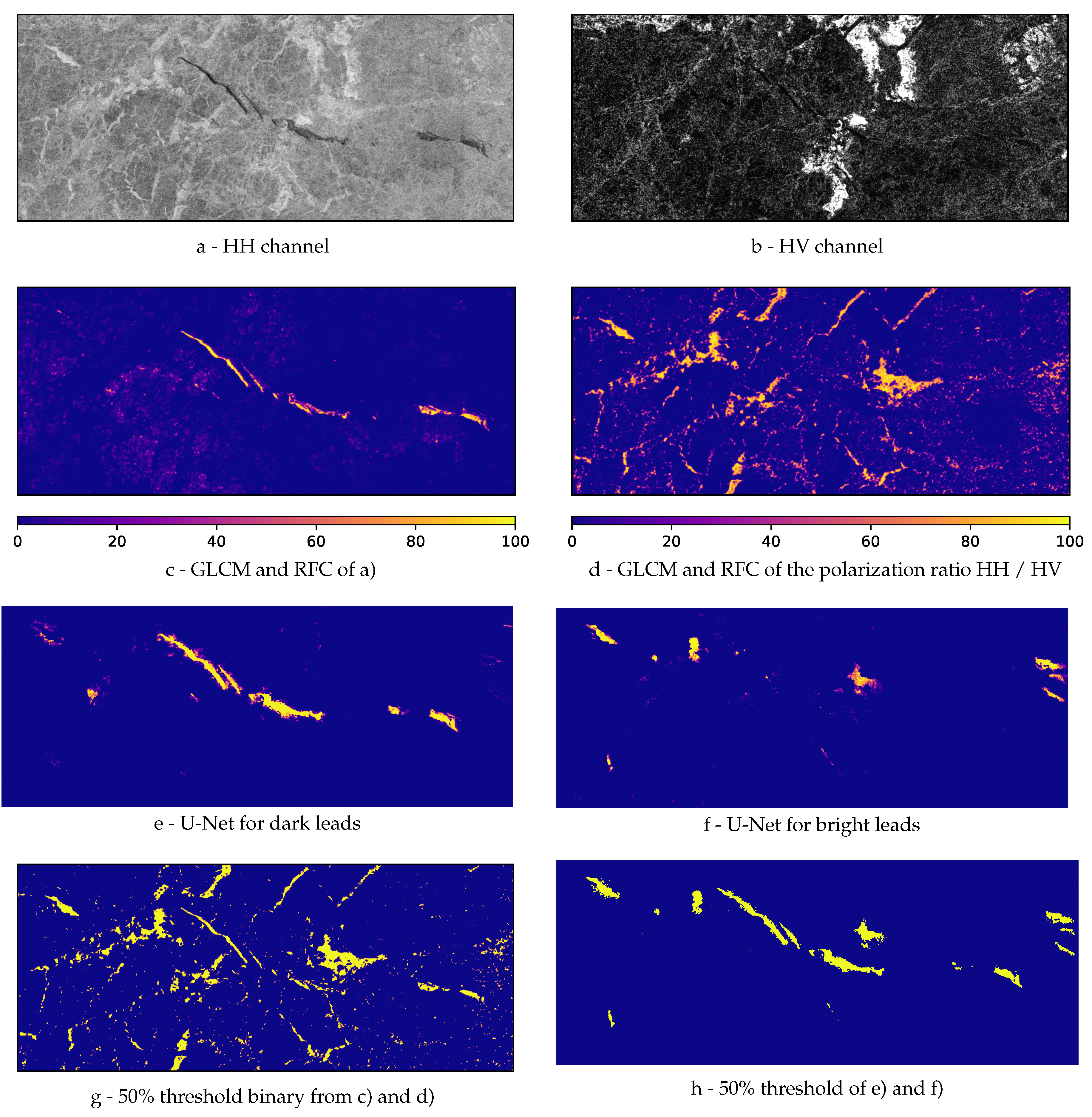
A detailed illustration of the lead detection results for each stage of the improved lead detection algorithm including comparison with the previously suggested lead detection algorithm and binarization comparison is shown in Figure 6. A cutout of the original Sentinel-1 scene taken on 2 January 2019 over the Chukchi Sea is shown in Figure 6a (HH channel) and Figure 6b (HV channel). As the first step, the lead detection algorithm is applied to the input image consisting of two channels. The probabilistic classification results for the previously suggested algorithm in [28] (GLCM and RFC) are shown in Figure 6c,d, results for the algorithm described in Section 2.3 of the present paper (U-Net -based) are shown in Figure 6e,f. Figure 6g shows binary classification with the 50% threshold applied to the previous GLCM and RFC results in Figure 6c,d. Binary classifications for the improved U-Net -based classification is shown in Figure 6h.

The classification quality is evaluated by applying the classification to 18 manually labeled Sentinel-1 scenes, which have not been used for training or testing. The classification accuracy on the evaluation data is 99.2%. The normalized confusion matrix is shown in Table 1. Both the accuracy score and the confusion matrix are weighted by number of class samples. This is done to ensure, that each class has the same contribution in the evaluation scores. It is important in case unbalanced amount of class samples and the number of lead pixels is naturally significantly lower than number of sea ice pixels.

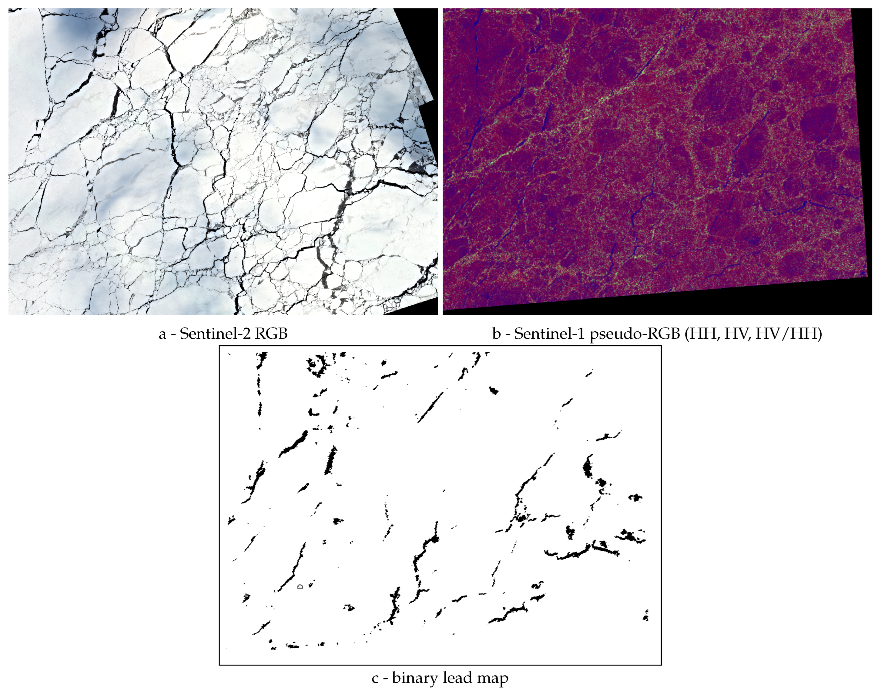
We compare a classified SAR scene with the Sentinel-2 optical image acquired on the same day in Figure 7. Sentinel-1 SAR and Sentinel-2 optical images were acquired on 21 March 2019 with a 7-hour time difference. Despite changes in the ice field between the SAR and the optical image (Figure 7a,b), the major cracks are recognizable on both images and are detected with the lead detection algorithm Figure 7c. However, many small leads visible in the Sentinel-2 image are not recognizable in the Sentinel-1 image and, therefore, are not detected. The SAR classification shows little false positives but can produce false negative lead results, see the confusion matrix in Table 1.

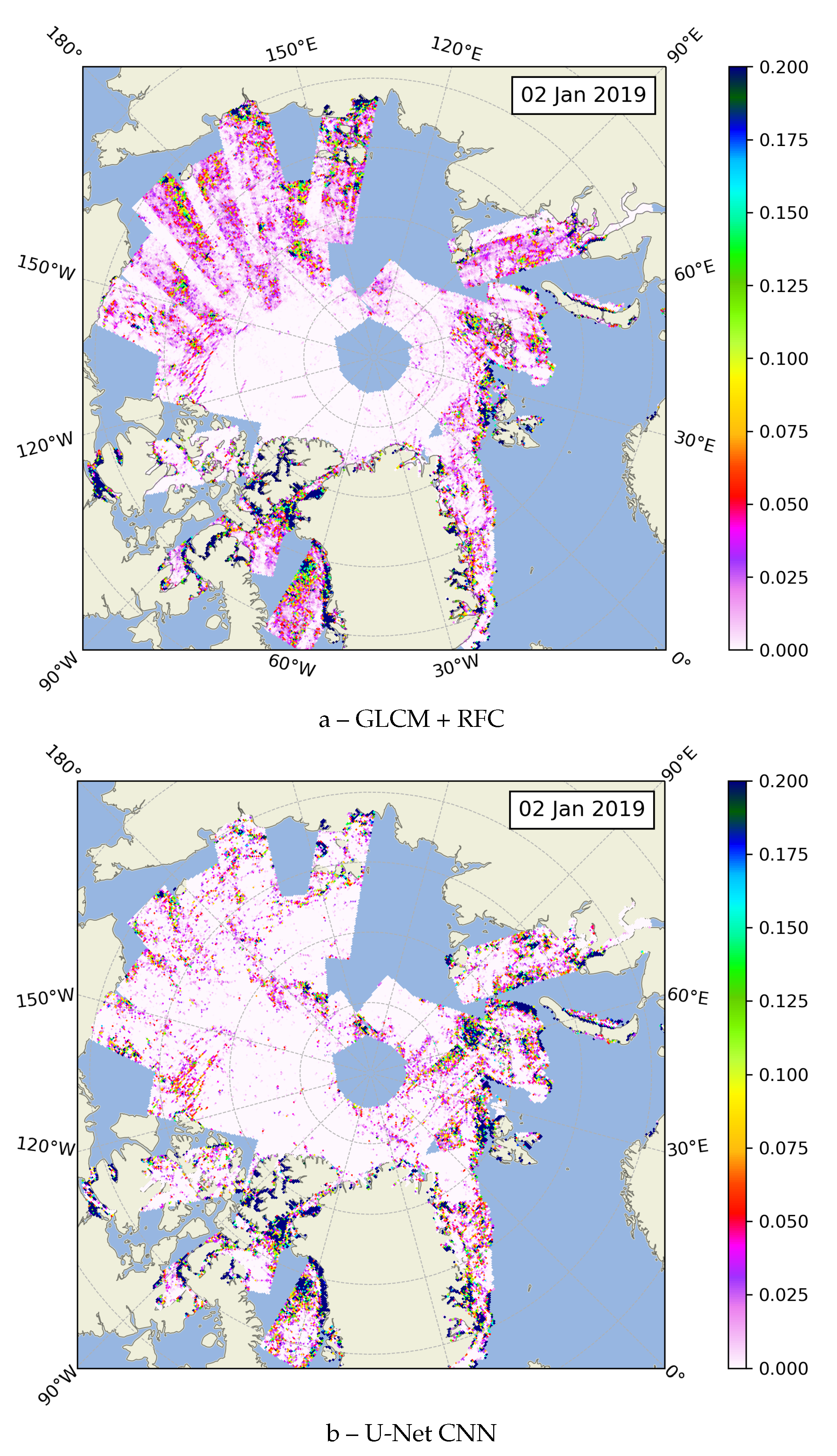
To see the large-scale picture, we have applied the improved lead detection algorithm to all Sentinel-1 scenes acquired over the Arctic on 2 January 2019. The binary lead classification on individual SAR scenes are merged together to produce a pan-Arctic lead map. In case when scenes overlap, the information from the latest acquired scene is used. The lead information is then available at the Sentinel-1 EW native 40 meter pixel size Arctic-wide for all regions covered by Sentinel-1 SAR (full coverage with two satellites takes about three days). The high resolution and extent of the map does not allow us to present it here in full detail as a figure. Therefore, we calculate the lead area fraction on a 12 km grid, for representation of the 40 m resolution lead maps as an image. An Arctic-wide comparison of lead detection results is shown in Figure 8. The two images Figure 8a,b correspond to images Figure 6g,h of the fine scale comparison. That is, Figure 8a represents the result of the previous lead detection algorithm from [28], Figure 8b is the result of the new U-Net based lead detection with 50% threshold applied. The lead map in Figure 8b shows a more uniform distribution of leads over the Arctic without apparently artificial higher lead fractions along the swath edges. Areas with higher lead fraction like in the Beaufort Sea can clearly be identified despite the 12 km grid lead area averaging.

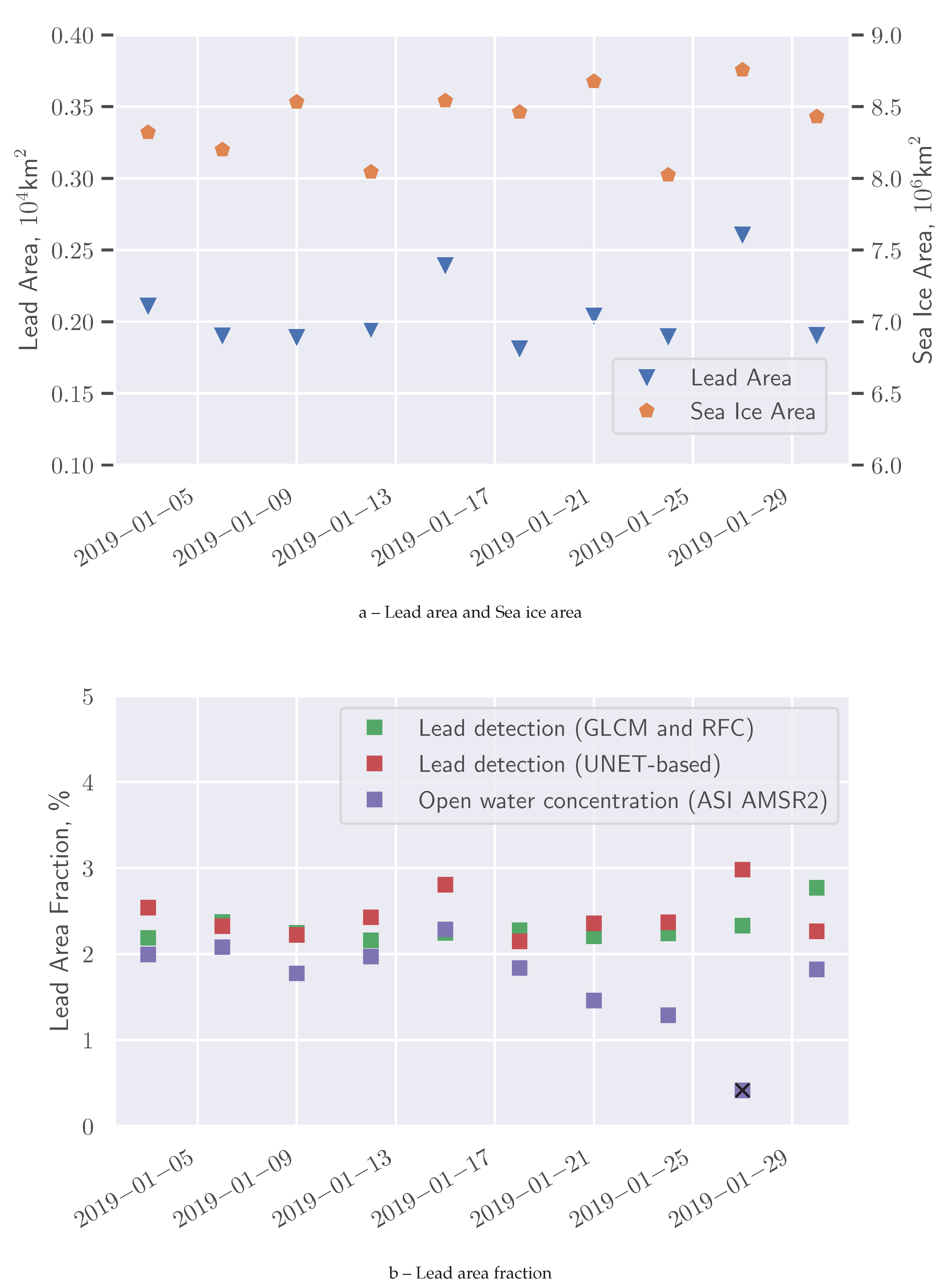
To ensure the algorithm produces stable results, we have applied it to all Sentinel-1 scenes taken over the Arctic in January 2019. Daily lead maps are combined into 3-day composite maps to decrease amount of gaps where no Sentinel-1 data was acquired. In case of overlapping Sentinel-1 scenes, the newer scene is always preferred for the overlap. A sea ice mask based on passive microwave sea ice concentration from AMSR2 [30] (seaice.uni-bremen.de) is applied. In order to derive the sea ice mask, first sea ice concentration data at 6.250 km resolution is resampled to 400 m with linear interpolation, after that a 15% threshold is applied. The resulting binary mask is resampled to 40 m and then applied to the 3-day composite maps. To avoid the influence of sub-daily change in sea ice conditions on the estimate for the lead area fraction, the sea ice mask is shrunk by 10 km in the marginal ice areas with morphological binary erosion. Therefore, marginal ice areas where sea ice extent is smaller on Sentinel-1 scenes compared to the corresponding AMSR2 data, which happens when sea ice retreats within the acquisition time window between the satellites and results in increased open water fraction at the ice edge, are not accounted as leads in further analysis. The total lead area and the sea ice area are calculated pixel-wise (40 m pixel size) for each 3-day composite map and are shown in Figure 9a. The ratio of the two is presented in Figure 9b in red. Figure 9b also shows lead area fraction derived with the previous lead detection algorithm (in green) and open water concentration calculated from the passive microwave sea ice concentration maps, cut to the coverage of Sentinel-1 scenes for the corresponding days. All three are calculated on the same extent: areas covered with Sentinel-1 acquisitions and considered as ice-covered areas with AMSR2 data. According to the improved U-Net -based lead detection, the mean lead area fraction in January 2019 is 2.44% with a standard deviation of 0.25 for the 10 data points of the time series, whereas the previous GLCM and RFC algorithm shows a mean lead area fraction of 2.30% with standard deviation 0.17. The open water concentration on AMSR2 data is 1.83% with 0.29 standard deviation. The AMSR2 data on 27 January 2019 has gaps in the Arctic coverage providing smaller open water concentration and is, therefore, considered as outlier and excluded from calculations. Small variations in lead area and sea ice area may appear due to natural reasons, which include lead opening, closing, and refreezing, as well as due to small differences in satellite coverage since sometimes the Arctic is not entirely covered even on 3-day composite maps. Overall, the lead area fraction is stable throughout the month, as can be expected for January in the middle of winter. This hints to the fact that the SAR lead classification can produce stable lead area fraction estimates.

4. Discussion

The sub-swath balancing technique described in Section 2.2 adjusts the thermal noise by sub-swath and removes the sudden changes in backscatter between sub-swaths over a uniform surface, which are very noticeable at swath borders, as shown in Figure 2. This leads to a smaller, more natural backscatter variation in the HV channel, making it more reliable for use as input for automatic classification algorithms.

On one hand, the classification results shown in Figure 6 illustrate the improvement of the U-Net -based lead detection algorithm over the previously suggested GCLM and RFC method. On the one hand, leads are detected with more confidence (see Figure 6c–f, scale shows probability of a pixel to be detected as lead), on the other hand less objects appearing due to scalloping and speckle noise are present in the classified images. This is especially noticeable for bright leads, that have preciously been detected from the polarization ratio, which, in turn, had a greater influence of thermal noise. The swath balancing technique described in Section 2.2 decreases variation in HV backscatter values appearing due to thermal noise, as shown in Figure 2.

The Arctic-wide lead maps (Figure 8) show a clear improvement in lead detection in the Siberian region of the Arctic. This is the region of thin and flat ice, which has a low backscatter values. A scene preprocessing that provides a robust backscatter across Sentinel-1 scenes in the area is essential. While the previously suggested algorithm based on GLCM features by the insufficient subswath correction, the new method based on U-Net is not. The U-Net -based lead detection algorithm described in Section 2.3 shows a significant improvement in performance. While the GLCM and RFC algorithm could only be applied to the European Arctic, the proposed method works over the entire Arctic.

The lead area and the sea ice area calculated on 3-day composite map are correlated as shown in Figure 9a with the correlation coefficient of 0.56. This indicates that the variations in the total lead area partly come from the variability of Sentinel-1 coverage. The difference in coverage between 3-day time steps should therefore have little influence on the lead area fraction calculated as a ratio of the lead area to the sea ice area. In this study, 3-day composite lead maps are produces with the data retrieved from the two satellites Sentinel-1A and Sentinel-1B. With only one satellite available (as it is currently the case in 2024) the coverage in the Arctic is reduced significantly. Due to changes in the acquisition plan some areas may be covered at the same temporal frequency (for instance the European Arctic), other areas might be covered at much lower frequencies or not be covered at all.

In Figure 9b we demonstrate that the new algorithm delivers stable results: the lead area fraction (plotted in red) for January 2019 shows small variation with 0.25% standard deviation around its average value of about 2.44%. It is in the same range with the passive microwave open water concentration. The previously suggested algorithm shows little correlation with the AMSR2 data (0.05), but the correlation between the lead area fraction derived with the proposed U-Net -based algorithm and the AMSR2 open water fraction is significant, 0.49. The higher lead area fraction derived from SAR images is expected as the SAR lead class contains leads with open water and thin ice. The AMSR2 point on 2019-01-27 is an outlier due to reduced coverage on that date. This is one of a few days, when AMSR2 data does not cover the entire Arctic, so that the lead area fraction is lower than what it would be with the full coverage.

The open water concentration in the central Arctic away from marginal ice area is known to be typically around 1–3% [1,4,41]. In-situ observations of sea ice thickness in the Central Arctic indicate sea ice cover consists of 1% 0-20 cm thick sea ice (by area) [42]. Thus, the 2.44% lead area fraction derived with the improved lead detection algorithm is comparable to the previous studies. A slightly higher lead area fraction compared to passive microwave data may be related to a different sensitivity of C-band SAR data to thin ice. Conceptually the AMSR2 sea ice concentration should only show open water areas, while the Sentinel-1 lead map contains open water and thin ice. Thus it is reasonable that the AMSR2 open water fraction is smaller than the lead area fraction derived from SAR scenes.

As future steps, the suggested algorithm can be applied to a wider range of Sentinel-1 scenes to produce 40 m resolution pan-Arctic binary lead maps from 2016 until today. These maps can be analyzed on the lead distribution across the Arctic and frequency of lead occurrence in various Arctic regions can be computed. The shape of the detected leads can be analyzed and from that the distributions of the lead width, lead length, lead area, lead orientation can be derived both Arctic-wide and regionally. The temporal evolution of the total lead area beyond the one month presented here is subject of a followup study. Initial results on the lead maps analysis for five winter seasons 2016–2021 are available in [43].

5. Conclusions

We have described an improved preprocessing method for Sentinel-1 EW scenes, which balances sub-swath backscatter by sub-swath -wise scaling of thermal noise. We have introduced an improved lead detection algorithm for Sentinel-1 SAR scenes based on modified a U-Net convolutional neural network architecture. The results are evaluated using manually classified SAR scenes and in comparison to an optical Sentinel-1 scene. As the result, we are able to produce 3-day composite lead maps of the entire Arctic with 40 meter spatial resolution. Despite a lower temporal coverage compared to passive microwave measurements which provide a daily sea ice concentration map, the Sentinel-1 based lead map has unprecedentedly high resolution over the entire Arctic, independently of cloud and weather conditions. No other satellite delivers such high spatial resolution for all weather conditions. The average lead concentration in January 2019 of 2.44% is slightly higher than the one derived from passive microwave sea ice concentration measurement, which is expected as many leads are smoothed out on AMSR2 data due to its considerably lower resolution (6.25 km versus 40 meters of Sentinel-1) and the fact that the AMSR2 lead area only contains open water while our SAR-based lead class also contains thin ice. With recently launched SAR missions (e.g., Radarsat Constellation Mission) and planned SAR missions (further Sentinel-1 satellites; ROSE-L mission) Arctic-wide SAR lead maps can be expected to be provided on a daily or sub-daily basis in the near future.

Acknowledgments

This study was supported by the Deutsche Forschungsgemeinschaft (DFG, German Research Foundation) through the International Research Training Group IRTG 1904 ArcTrain (grant 221211316), and the Transregional Collaborative Research Center TRR 172 “Arctic Amplification: Climate Relevant Atmospheric and Surface Processes, and Feedback Mechanisms (AC)³” (grant 268020496). We gratefully acknowledge the provision of Copernicus Sentinel-1 data [2018-2021] provided by the European Union via the Copernicus Open Access Hub (https://scihub.copernicus.eu).

References

Lindsay, R.W.; Rothrock, D.A. Arctic Sea Ice Leads from Advanced Very High Resolution Radiometer Images. Journal of Geophysical Research 1995, 100, 4533–4544. [Google Scholar] [CrossRef]
Reiser, F.; Willmes, S.; Heinemann, G. A New Algorithm for Daily Sea Ice Lead Identification in the Arctic and Antarctic Winter from Thermal-Infrared Satellite Imagery. Remote Sensing 2020, 12, 1957. [Google Scholar] [CrossRef]
Hoffman, J.P.; Ackerman, S.A.; Liu, Y.; Key, J.R.; McConnell, I.L. Application of a Convolutional Neural Network for the Detection of Sea Ice Leads. Remote Sensing 2021, 13, 4571. [Google Scholar] [CrossRef]
Röhrs, J.; Kaleschke, L. An Algorithm to Detect Sea Ice Leads by Using AMSR-E Passive Microwave Imagery. The Cryosphere 2012, 6, 343–352. [Google Scholar] [CrossRef]
Wernecke, A.; Kaleschke, L. Lead Detection in Arctic Sea Ice from CryoSat-2: Quality Assessment, Lead Area Fraction and Width Distribution. The CryosphereCryosphere 2015, 9, 1955–1968. [Google Scholar] [CrossRef]
Longepe, N.; Thibaut, P.; Vadaine, R.; Poisson, J.C.; Guillot, A.; Boy, F.; Picot, N.; Borde, F. Comparative Evaluation of Sea Ice Lead Detection Based on SAR Imagery and Altimeter Data. IEEE Transactions on Geoscience and Remote Sensing 2019, 57, 4050–4061. [Google Scholar] [CrossRef]
Ivanova, N.; Rampal, P.; Bouillon, S. Error Assessment of Satellite-Derived Lead Fraction in the Arctic. The Cryosphere 2016, 10, 585–595. [Google Scholar] [CrossRef]
Komarov, A.S.; Buehner, M. Adaptive Probability Thresholding in Automated Ice and Open Water Detection from RADARSAT-2 Images. IEEE Geoscience and Remote Sensing Letters 2018, 15, 552–556. [Google Scholar] [CrossRef]
Linow, S.; Dierking, W. Object-Based Detection of Linear Kinematic Features in Sea Ice. Remote Sensing 2017, 9, 1–15. [Google Scholar] [CrossRef]
Hutter, N.; Zampieri, L.; Losch, M. Leads and Ridges in Arctic Sea Ice from RGPS Data and a New Tracking Algorithm. Cryosphere 2019, 13, 627–645. [Google Scholar] [CrossRef]
Von Albedyll, L.; Hendricks, S.; Hutter, N.; Murashkin, D.; Kaleschke, L.; Willmes, S.; Thielke, L.; Tian-Kunze, X.; Spreen, G.; Haas, C. Lead Fractions from SAR-derived Sea Ice Divergence during MOSAiC. The Cryosphere 2024, 18, 1259–1285. [Google Scholar] [CrossRef]
Komarov, A.S.; Landy, J.C.; Komarov, S.A.; Barber, D.G. Evaluating Scattering Contributions to C-Band Radar Backscatter From Snow-Covered First-Year Sea Ice at the Winter – Spring Transition Through Measurement and Modeling. IEEE Transactions on Geoscience and Remote Sensing 2017, 55, 5702–5718. [Google Scholar] [CrossRef]
Fors, A.S.; Member, S.; Brekke, C.; Gerland, S.; Doulgeris, A.P.; Beckers, J.F.; Member, S. Late Summer Arctic Sea Ice Surface Roughness Signatures in C-Band SAR Data. IEEE Journal of Selected Topics in Applied Earth Observations and Remote Sensing 2016, 9, 1199–1215. [Google Scholar] [CrossRef]
Ressel, R.; Singha, S.; Lehner, S.; Rosel, A.; Spreen, G. Investigation into Different Polarimetric Features for Sea Ice Classification Using X-Band Synthetic Aperture Radar. IEEE Journal of Selected Topics in Applied Earth Observations and Remote Sensing 2016, 9, 3131–3143. [Google Scholar] [CrossRef]
Singha, S.; Johansson, M.; Hughes, N.; Hvidegaard, S.M.; Skourup, H. Arctic Sea Ice Characterization Using Spaceborne Fully Polarimetric L-, C-, and X-Band SAR with Validation by Airborne Measurements. IEEE Transactions on Geoscience and Remote Sensing 2018, 56, 3715–3734. [Google Scholar] [CrossRef]
Xie, T.; Perrie, W.; Wei, C.; Zhao, L. Discrimination of Open Water from Sea Ice in the Labrador Sea Using Quad-Polarized Synthetic Aperture Radar. Remote Sensing of Environment 2020, 247, 111948. [Google Scholar] [CrossRef]
Zhao, L.; Xie, T.; Perrie, W.; Yang, J. Sea Ice Detection from RADARSAT-2 Quad-Polarization SAR Imagery Based on Co- and Cross-Polarization Ratio. Remote Sensing 2024, 16, 515. [Google Scholar] [CrossRef]
Leigh, S.; Wang, Z.; Clausi, D.A. Automated Ice-Water Classification Using Dual Polarization SAR Satellite Imagery. IEEE Transactions on Geoscience and Remote Sensing 2014, 52, 5529–5539. [Google Scholar] [CrossRef]
Liu, H.; Guo, H.; Zhang, L. SVM-Based Sea Ice Classification Using Textural Features and Concentration From RADARSAT-2 Dual-Pol ScanSAR Data. IEEE Journal of Selected Topics in Applied Earth Observations and Remote Sensing 2015. [Google Scholar] [CrossRef]
Zakhvatkina, N.; Korosov, A.; Muckenhuber, S.; Sandven, S.; Babiker, M. Operational Algorithm for Ice–Water Classification on Dual-Polarized RADARSAT-2 Images. The Cryosphere 2017, 11, 33–46. [Google Scholar] [CrossRef]
Li, X.M.; Sun, Y.; Zhang, Q. Extraction of Sea Ice Cover by Sentinel-1 SAR Based on Support Vector Machine with Unsupervised Generation of Training Data. IEEE Transactions on Geoscience and Remote Sensing 2021, 59, 3040–3053. [Google Scholar] [CrossRef]
Qu, M.; Lei, R.; Liu, Y.; Li, N. Arctic Sea Ice Leads Detected Using Sentinel-1B SAR Image and Their Responses to Atmosphere Circulation and Sea Ice Dynamics. Remote Sensing of Environment 2024, 308, 114193. [Google Scholar] [CrossRef]
Boulze, H.; Korosov, A.; Brajard, J. Classification of Sea Ice Types in Sentinel-1 SAR Data Using Convolutional Neural Networks. Remote Sensing 2020, 12, 2165. [Google Scholar] [CrossRef]
Chen, X.; Patel, M.; Pena Cantu, F.J.; Park, J.; Noa Turnes, J.; Xu, L.; Scott, K.A.; Clausi, D.A. MMSeaIce: A Collection of Techniques for Improving Sea Ice Mapping with a Multi-Task Model. The Cryosphere 2024, 18, 1621–1632. [Google Scholar] [CrossRef]
Malmgren-Hansen, D.; Pedersen, L.T.; Nielsen, A.A.; Kreiner, M.B.; Saldo, R.; Skriver, H.; Lavelle, J.; Buus-Hinkler, J.; Krane, K.H. A Convolutional Neural Network Architecture for Sentinel-1 and AMSR2 Data Fusion. IEEE Transactions on Geoscience and Remote Sensing 2021, 59, 1890–1902. [Google Scholar] [CrossRef]
Wang, Y.R.; Li, X.M. Arctic Sea Ice Cover Data from Spaceborne Synthetic Aperture Radar by Deep Learning. Earth System Science Data 2021, 13, 2723–2742. [Google Scholar] [CrossRef]
Liang, Z.; Pang, X.; Ji, Q.; Zhao, X.; Li, G.; Chen, Y. An Entropy-Weighted Network for Polar Sea Ice Open Lead Detection From Sentinel-1 SAR Images. IEEE Transactions on Geoscience and Remote Sensing 2022, 60, 1–14. [Google Scholar] [CrossRef]
Murashkin, D.; Spreen, G.; Huntemann, M.; Dierking, W. Method for Detection of Leads from Sentinel-1 SAR Images. Annals of Glaciology 2018, 59, 124–136. [Google Scholar] [CrossRef]
Ronneberger, O.; Fischer, P.; Brox, T. U-Net: Convolutional Networks for Biomedical Image Segmentation, 2015, [arXiv:cs/1505.04597]. [CrossRef]
Spreen, G.; Kaleschke, L.; Heygster, G. Sea Ice Remote Sensing Using AMSR-E 89-GHz Channels. Journal of Geophysical Research 2008, 113. [Google Scholar] [CrossRef]
Tomasi, C.; Manduchi, R. Bilateral Filtering for Gray and Color Images. Sixth International Conference on Computer Vision, 1998. [CrossRef]
Haralick, R.M.; Shanmugam, K.; Dinstein, I. Textural Features for Image Classification. IEEE Transactions on Systems, Man, and Cybernetics 1973, smc-3, 610–621. [Google Scholar] [CrossRef]
Ho, T.K. The Random Subspace Method for Constructing Decision Forests. IEEE Transactions on Pattern Analysis and Machine Intelligence 1998, 20, 832–844. [Google Scholar] [CrossRef]
Breiman, L. Random Forests. Machine Learning 2001, 45, 5–32. [Google Scholar] [CrossRef]
Park, J.W.; Won, J.S.; Korosov, A.A.; Babiker, M.; Miranda, N. Textural Noise Correction for Sentinel-1 TOPSAR Cross-Polarization Channel Images. IEEE Transactions on Geoscience and Remote Sensing 2019, 57, 4040–4049. [Google Scholar] [CrossRef]
Sun, Y.; Li, X.M. Denoising Sentinel-1 Extra-Wide Mode Cross-Polarization Images Over Sea Ice. IEEE Transactions on Geoscience and Remote Sensing 2021, 59, 2116–2131. [Google Scholar] [CrossRef]
Korosov, A.; Demchev, D.; Miranda, N.; Franceschi, N.; Park, J.W. Thermal Denoising of Cross-Polarized Sentinel-1 Data in Interferometric and Extra Wide Swath Modes. IEEE Transactions on Geoscience and Remote Sensing 2022, 60, 1. [Google Scholar] [CrossRef]
Hinton, G.E.; Srivastava, N.; Krizhevsky, A.; Sutskever, I.; Salakhutdinov, R.R. Improving Neural Networks by Preventing Co-Adaptation of Feature Detectors, 2012, [arXiv:cs/1207.0580].
Fukushima, K. Visual Feature Extraction by a Multilayered Network of Analog Threshold Elements. IEEE Transactions on Systems Science and Cybernetics 1969, 5, 322–333. [Google Scholar] [CrossRef]
Cortes, C.; Mohri, M.; Rostamizadeh, A. L2 Regularization for Learning Kernels 2009.
Maykut, G.A. Energy Exchange over Young Sea Ice in the Central Arctic. Journal of Geophysical Research 1978, 83, 3646–3658. [Google Scholar] [CrossRef]
Thorndike, A.S.; Rothrock, D.A.; Maykut, G.A.; Colony, R. The Thickness Distribution of Sea Ice. Journal of Geophysical Research 1975, 80, 4501–4513. [Google Scholar] [CrossRef]
Murashkin, D. Remote Sensing of Sea Ice Leads with Sentinel-1 C-band Synthetic Aperture Radar 2024. [CrossRef]

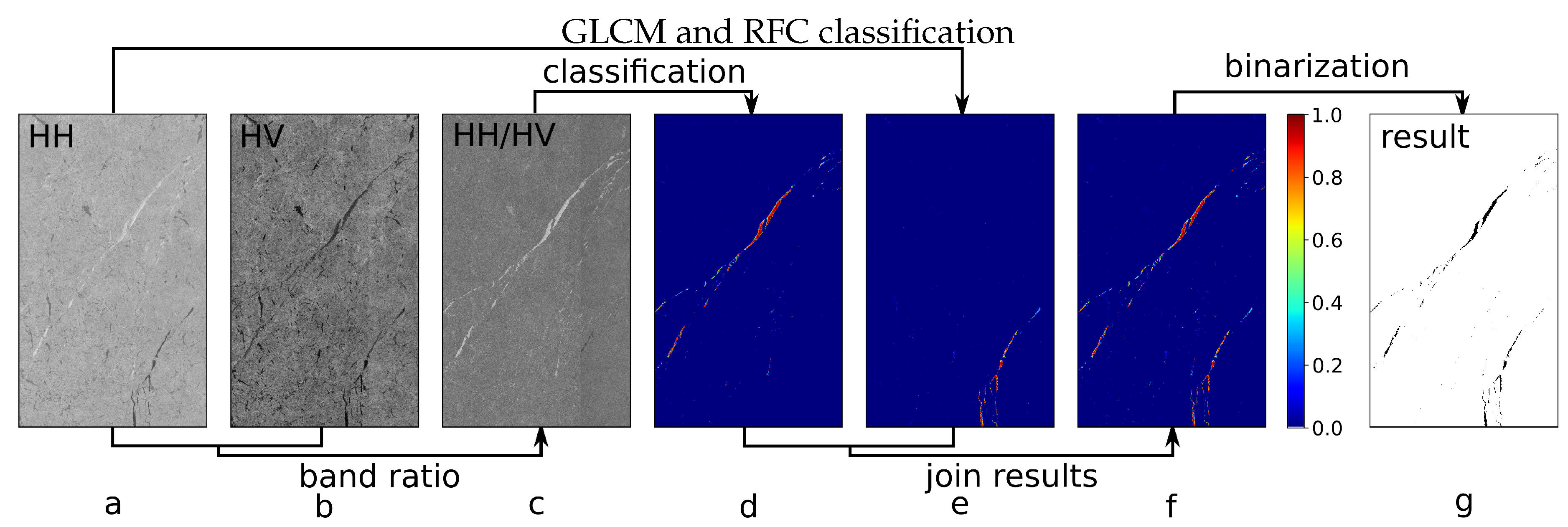
Figure 1. Lead detection algorithm based on Gray-Level Co-Occurrence Matrix (GLCM) features using a Random Forest Classifier (RFC) as presented in [28]. (a) and (b) are the original Sentinel-1 SAR data (3 Feb 2016, 22:29, Canadian Arctic; size of the area shown is about 150 km by 80 km), HH and HV respectively. (c) is the band ratio HH/HV. (d) and (e) are lead probabilities produced by the lead classification algorithm for the HH channel and the polarization ratio, corresponds to (a) and (c). GLCM calculation and RFC are used on this step. (f) is the sum of probabilities (d) and (e). (g) is the binary classification derived from (f) by applying a threshold of 50%.

Figure 2. Example of preprocessing for two Sentinel-1 scenes on 2d January 2019 over Beaufort Sea (left column) and Franz Josef land (right column). Here only HV channels are shown as the noise on the HH channel is less notable due to higher backscatter values. (a) and (b) basic preprocessing result using the noise data provided with each scene as meta data; (c) and (d) improved preprocessing result with noise scaling for each sub-swath applied; (e) and (f) mean NRCS values along azimuth direction, for the basic preprocessing a), b) in blue, and for the improved preprocessing algorithm c), d) in orange.

Figure 3. The U-Net-based architecture used in the study: the number of layers has been extended to 6 layers compared to 4 layers in the original U-Net architecture, input tile size has been set to 512×512 pixels, padding is set to "same" so that the output image has the size of the input image.

Figure 4. Smooth prediction for edge effects reduction from U-Net tiles. A trained model is applied to a given SAR scene four times, each time with an offset. Zero offset is shown in black, 25% offset is red, 50% offset is green, 75% offset is blue. A pixel of a tile (shown in purple) appears close to the center of the tile in case of red tiling and close to the edge on the blue tiling.

Figure 5. Improved lead detection algorithm based on a U-Net convolutional neural network. (a) and (b) are the original Sentinel-1 SAR data (3 Feb 2016, 22:29, Canadian Arctic; size of the area shown is about 150 km by 80 km), HH and HV channels respectively. (c) and (d) are lead probabilities produced by the lead classification algorithm for dark and bright leads, based on (a) and (b). U-Net convolutional neural network is used at this step. (e) is the sum of probabilities (c) and (d). (f) is the binary classification derived from (e) by applying a threshold of 50%.

Figure 6. Example of lead classification: a and b - raw data, HH and HV SAR channels; c and d - previous probabilistic lead classifications (GLCM and RFC) for dark (HH channel) and bright (polarization ratio) leads; e and f - probabilistic lead classification produced with the improved lead detection algorithm (U-Net); g - binary classification calculated by applying a 50% threshold to the GLCM and RFC probabilistic classifications c and d; h - binary classification calculated by applying a 50% threshold to the U-Net probabilistic classifications e and f; The scene was taken on 2 January 2019 over the Chukchi Sea, the scene name is "S1B_EW_GRDM_1SDH_20190102T190125_20190102T190220_014319_01AA45_7719"

Figure 7. (a) Sentinel-2 optical RGB image has been acquired on 21 of March 2019 at 9:17UTC, (b) Sentinel-1 SAR pseudo-RBG (HH, HV, HV/HH) has been acquired on 21 of March 2019 at 2:32UTC, (c) Result of the lead detection algorithm applied to scene b).

Figure 8. Pan-Arctic Lead Area Fraction maps (12 km resolution) derived from the daily Arctic lead map. The Arctic lead map consists of all Sentinel-1 scenes acquired over the Arctic on 2 Jan 2019. (a) Lead Area Fraction derived with the previous algorithm based on GLCM features and Random Forest classifier as described in [28]. (b) Lead Area Fraction derived with the improved lead detection algorithm based on U-Net CNN.

Figure 9. (a) Lead area (left y-axis) and sea ice area (right y-axis)), and (b) lead area fraction derived from 3-day composite lead maps of the Arctic in January 2019. The sea ice area in (a) mainly changes due to changing satellite coverage (i.e., not due to ice growth/melting).

Table 1. Normalized confusion matrix for the lead detection algorithm. i-th row and j-th column entry indicates the number of samples with true label being i-th class and predicted label being j-th class.

true\predicted	dark leads	bright leads	sea ice
dark leads	0.989	0.0	0.011
bright leads	0.0	0.989	0.011
sea ice	0.001	0.0	0.999

Disclaimer/Publisher’s Note: The statements, opinions and data contained in all publications are solely those of the individual author(s) and contributor(s) and not of MDPI and/or the editor(s). MDPI and/or the editor(s) disclaim responsibility for any injury to people or property resulting from any ideas, methods, instructions or products referred to in the content.

© 2024 by the authors. Licensee MDPI, Basel, Switzerland. This article is an open access article distributed under the terms and conditions of the Creative Commons Attribution (CC BY) license (http://creativecommons.org/licenses/by/4.0/).

Copyright: This open access article is published under a Creative Commons CC BY 4.0 license, which permit the free download, distribution, and reuse, provided that the author and preprint are cited in any reuse.

MDPI Initiatives

Important Links

Choose an area of interest and we will send you notifications of new preprints at your preferred frequency.

Disclaimer