Ensemble based Machine Learning Algorithm for Loan Default Risk Prediction

1. Introduction

Numerous financial institutions, like banks and lending platforms have relied on the interest and fees from loans as a source of revenue [1], so, to maintain their financial strength and profitability, banks and lending platforms must ensure that the loan payments are made and that borrowers do not default on their payments. Although the economic breakdown in the late 2000s, specifically the financial crisis in 2008, was caused by many factors, it can also highlight the impact of lending to individuals or businesses who are unable to repay their debts [2,3], which is why predicting credit default risk is important, as it can help lenders avoid having large losses, mitigate financial crises and further maintain public trust in the banking system [4]. Therefore, credit default risk is the likelihood that a borrower will fail to fulfil their payment obligations [5,6,7].

Hence, given the need to accurately predict credit default risk, this study aims to compare various machine learning models for this prediction. This study further combines these models with boosting classifiers, such as eXtreme Gradient Boosting (XGBoost) and ADAptive Boosting (ADABoost), to determine if the combined or ensembled model will perform better than the individual models. By evaluating how accurate the models are at predicting defaults, this project seeks to determine the most effective technique to accurately assess credit default risk using dataset from LendingClub [8], a financial lending company, which includes detailed information on every loan issued from 2007 to 2018, including the comprehensive list of borrowers’ characteristics, such as their annual income, amount borrowed, loan purpose, debt-to-income ratio, credit history, credit score and other relevant variables.

Furthermore, literature synthesis evidenced that a common problem in credit default prediction is the issue of class imbalance. Therefore, this paper handled class imbalance by testing various techniques, including over-sampling techniques such as Random Over-Sampling (ROS), Synthetic Minority Oversampling Technique (SMOTE) and Adaptive Synthetic Sampling (ADASYN), under-sampling techniques such as Random Under-Sampling (RUS) and Tomek Links, as well as a combination of sampling techniques such as SMOTE Tomek and SMOTE with the Edited Nearest Neighbours (SMOTE + ENN).

The methodology followed by [9] is the closest to the methodology used in this work and we were able to achieve higher result compared to the accuracy obtained by the study [9], as well as in comparison to these related studies [10,11,12]. This study is arranged as follows, with the subsequent section exploring existing techniques and methodologies related to credit default prediction (Section 2), followed by the methodology made use of in this study (Section 3), then the results obtained (Section 4), finally, the conclusion and recommendations (Section 5).

2. Related Works

Authors in [13] showed that loan default rate and profitability are highly correlated and thus, models that can be used to accurately predict loan default is required, which is why machine learning techniques have been taken advantage of, as they have significantly improved the performance of predictability in various financial applications [14-17]. In the context of credit default prediction, the data used contains various borrowers’ characteristics as inputs and the target variable, therefore, this study does not consider the use of unsupervised learning algorithms for the prediction of default.

Several supervised machine learning models such as logistic regression, random forest, decision tree, Support Vector Machine (SVM), Multilayer Perceptron (MLP), Extreme Gradient Boosting (XGBoost) and Adaptive Boosting (ADABoost) have been used for credit default prediction. However, very few studies have thoroughly addressed the issue of class imbalance which limits the generalisation of the models. For example, the study of [14] compared SVM and logistic regression models to predict credit default, using data from the portfolio of a Portuguese bank. Their study achieved good results using SVM, however, the size of the dataset (1992 non-defaulting customers and 1008 defaulting customers) used may bring about some limitations. Similarly, authors in [1] made use of random forest and decision tree for their prediction. They showed random forest performed better than the decision tree with 80% accuracy. However, it is worth stating that their study evaluated the models mainly with accuracy. Unfortunately, the evaluation metric, accuracy is not sufficient for evaluation in the presence of class imbalance as the models are biased to the majority class, which in this case is the non-defaulters.

Similar to random forest used in [1], there are some machine learning models that are derived from the combination of predictions from multiple models using techniques like boosting, which is an ensemble technique that combines weak learners to create stronger algorithms [18]. For example, in [17], boosting classifiers, Light Gradient Boosting Machine (LightGBM) and XGBoost were used for the prediction of loan default using LendingClub data, from July 2007 to June 2017. This study had an interesting approach to cleaning the data, as in this study, two separate cleaning processes, multi-observational and multi-dimensional methods were used to identify and correct inconsistencies, observing that multi-observational was the superior method. With an accuracy of 80.1% and an error rate of 19.9%, the authors noted that LightGBM outperformed the XGBoost classifier in the prediction of loan defaults.

The prevalence of class imbalance in credit data was observed by [19], which is an issue that occurs when the classes in the dataset are not represented equally. In loan dataset, the non-default loans are usually more than the defaulted loans, and if not handled properly, it can cause the model to perform poorly on the minority class. [19] proposed XGBoost classifier to build credit risk assessment models and made use of cluster-based under-sampling to process the imbalanced data. Accuracy and the Area Under the Receiver Operating Characteristic Curve (AUC-ROC) was used as validation metrics, as the proposed model was compared with other models including logistic regression and SVM, with XGBoost outperforming the other models with an accuracy of 90.0% against 69.7% and 76.9% accuracy scores for logistic regression and SVM respectively, and AUC values of 0.94 against 0.77 and 0.87. Although this study achieved an impressive result with the proposed model, the dataset size might pose a limitation, as 6,271 records were used in this research. Additionally, even though the authors addressed the class imbalance issue, they focused only on using cluster-based under-sampling, without considering other techniques that might be more effective or suitable. Furthermore, the study of [20] made use of a deep learning model to predict consumer loan default using a dataset with 1,000 observations gotten from the response to a questionnaire created by the authors. This study used Keras, a neural network library which runs on TensorFlow. Although this research made use of a deep learning model in the prediction of bad loans, it is not directly comparable to this current study, given the mode of data collection, which involved selecting eleven top banks and distributing a survey to only participants who had taken out loans, which is significantly different from the dataset used in this current study. However, similar to this current study, [20] employed stratified random sampling.

The assessment and prediction of lending risk using MLP with three-hidden layers was presented by [21] with the LendingClub dataset used for the model development and evaluation. The authors classified the output variable into three categories using TensorFlow: safe loans, risky loans and bad loans, with majority of the data belonging to safe loan. The class imbalance issue was handled using Synthetic Minority Oversampling Technique (SMOTE). Furthermore, accuracy served as the measure of the model’s performance when compared with other models. The deep learning model with an accuracy of 93.2% outperformed other models including logistic regression (77.1%), decision tree (50.5%), linear SVM (78.9%), ADABoost (85.2%) and MLP with one-hidden layer (62.8%). The other performance metrics used were sensitivity (75.6%) and specificity (72.2%). In this study, no under-sampling or hybrid method was used to handle class imbalance.

Authors in [15] used Artificial Neural Network (ANN), random forest, XGBoost, and Gradient Boosting Regression Tree (GBRT). To address the issue of class imbalance, SMOTE was employed. In terms of the prediction models, GBRT constructs an ensemble of weak prediction trees to form a stronger predictor, while random forest obtains predictions by averaging the predictions from multiple individually trained decision trees. On the other hand, ANN is based on a mathematical process that can process nonlinear relationships between the independent variables and dependent variable. [15] showed that random forest model performed better than the other models when using metrics such as accuracy, kappa, precision, recall and F1-score to evaluate the performance of the models. The study of [16] used logistic regression and MLP models to predict credit default. Gini coefficient was used for feature selection, it measures the separation capability of the model. Subsequently, they combine the models with two ensemble techniques, the first method was averaging the probabilities obtained from both models to get the final predictions (bagging), while the second method was to input the probabilities into logistic regression (meta-model) to produce a final probability value. Bagging ensemble model performed better than all the other models, with the performance of each model evaluated using AUC, Gini index, KS, accuracy, error ratio, Positive Predictive Value (PPV), and Negative Predictive Value (NPV).

Authors in [9] used diverse oversampling and under sampling techniques and thereafter used two ensemble methods, bagging and stacking, as well as K-Nearest Neighbour (KNN), random forest, Logistic Model Tress (LMT) and Gradient Boosted Decision Trees (GBDT) model. Moreover, three datasets – Taiwan clients credit dataset with 30,000 observations and 6,636 defaults, South-German clients credit dataset with 1,000 observations and 300 defaults, and lastly, Belgium clients credit dataset with 284,299 observations (492 frauds) from September 2013, were used to build the models. Class imbalance was handled using near miss, cluster centroid and random under-sampling methods, additionally, Adaptive Synthetic Sampling (ADASYN), SMOTE, k-means SMOTE, borderline SMOTE, SMOTE Tomek and random oversampling method were tested. [9] noted that the oversampling techniques performed better than the under-sampling techniques and the GBDT method with SMOTE performed better than the other models using accuracy, precision, recall, F-measure, ROC curve and G-means. Although, this current study uses similar methodology as [9], this current study is different, as it identifies the best method to make use of at each stage and further ensembles the boosting classifiers with other machine learning models, as well as with MLP model (three-hidden layers).

In [11], SMOTE was applied to balance the data used to build a smart application for loan approval prediction, the data used was from Kaggle repository, and contained 806 observations and 12 features, which was used to train logistic regression, decision tree, random forest, SVM, KNN, Gaussian naïve bayes, ADABoost, dense neural networks, long short-term memory and recurrent neural networks, measuring their performance with accuracy, precision, recall and f1-score. Similar to this current study, the voting approach was used to combine the models, taking two approaches, firstly combining the predictions from all the models, and also combining three of the best performing models. [11] observed that the deep learning models were less effective when dealing with loan dataset compared to the traditional machine learning models, with the second approach outperforming the other models. Although [11] handled class imbalance, this current study test other sampling techniques, used more data for the prediction, additionally other techniques were explored to improve the models’ performance similar to [12] and [22], as feature selection techniques were used to optimise the models for credit default risk predictions. [12] used features extracted from convolution neural networks, as well as Pearson correlation and Recursive Feature Elimination (RFE) to select the best features to build a deep learning-optimised stacking model to predict joint loan risk, concluding that feature selection played a big part in the performance of the final stacking model with a 6% increase in joint loan approval. Conversely, [22] used only RFE to select the features used to develop fused logistic regression, random forest and Categorical Boosting (CatBoost) models using the blended method. Additionally, they balanced the loan dataset using ADASYN. Furthermore, the authors highlighted the impact of feature selection, with the fused model performing better than the individual models when evaluated on accuracy, recall and F1-score.

Finally, few studies performed hyperparameter tuning using GridSearchCV. For example, reference [10] used GridSearchCV to get the parameters to build ANN, logistic regression, random forest, SVM, decision tree, XGBoost, LightGBM and a 2-layered neural network for credit risk prediction, with XGBoost also serving as the model used to test the class balancing method, as well as to get the feature importance within the model. Additionally, to deal with class imbalance, the authors randomly sampled the default loans and non-default loans, thereby under-sampling the data. Accuracy, recall, precision and F1-score served as the performance evaluators of the models, with [10] identifying XGBoost as the best performing model. This study highlighted the effectiveness of GridSearchCV in model optimisation.

In conclusion, accurately detecting credit defaults remains a concern to financial institutions, especially the role it plays in reducing financial losses [23], and while previous studies have applied various machine learning algorithms to accurately predict credit defaults, the problem of class imbalance and generalisation remains. Furthermore, the combination of boosting classifiers, testing different sampling techniques, and validating the models with various performance metrics remains an area with room for improvement, therefore, this current paper aims to solve this issue with a slightly different approach and methodology with respect to the existing literature.

3. Methodology

This section discusses the methods used in this study, starting with the data collection process to the model deployment stage. The data collected was from LendingClub [24], which is a lending platform that provides detailed information of each loan that was issued from 2007 to 2018. Given the focus of this study, only the confirmed good and bad loans were used [25], therefore, the target is defined as:

$$\mathrm{Target}\left(\mathrm{y}\right)=\left\{\begin{array}{c}0\text{:} \mathrm{w}\mathrm{h}\mathrm{e}\mathrm{r}\mathrm{e}\mathrm{l}\mathrm{o}\mathrm{a}\mathrm{n}\mathrm{s}\mathrm{t}\mathrm{a}\mathrm{t}\mathrm{u}\mathrm{s}=\text{"}\mathrm{F}\mathrm{u}\mathrm{l}\mathrm{l}\mathrm{y}\mathrm{P}\mathrm{a}\mathrm{i}\mathrm{d}\text{"}\\ 1\text{:} \mathrm{w}\mathrm{h}\mathrm{e}\mathrm{r}\mathrm{e}\mathrm{l}\mathrm{o}\mathrm{a}\mathrm{n}\mathrm{s}\mathrm{t}\mathrm{a}\mathrm{t}\mathrm{u}\mathrm{s}=\text{"}\mathrm{C}\mathrm{h}\mathrm{a}\mathrm{r}\mathrm{g}\mathrm{e}\mathrm{d}\mathrm{o}\mathrm{f}\mathrm{f}\text{"}\end{array}\right.$$

(1)

To balance the system’s efficiency and have a representative of the data, 30% of the data was sampled using stratified sampling method [25], which resulted to a sample size of 403,593 and 152 variables. This approach ensured that there was sufficient data without overwhelming the system.

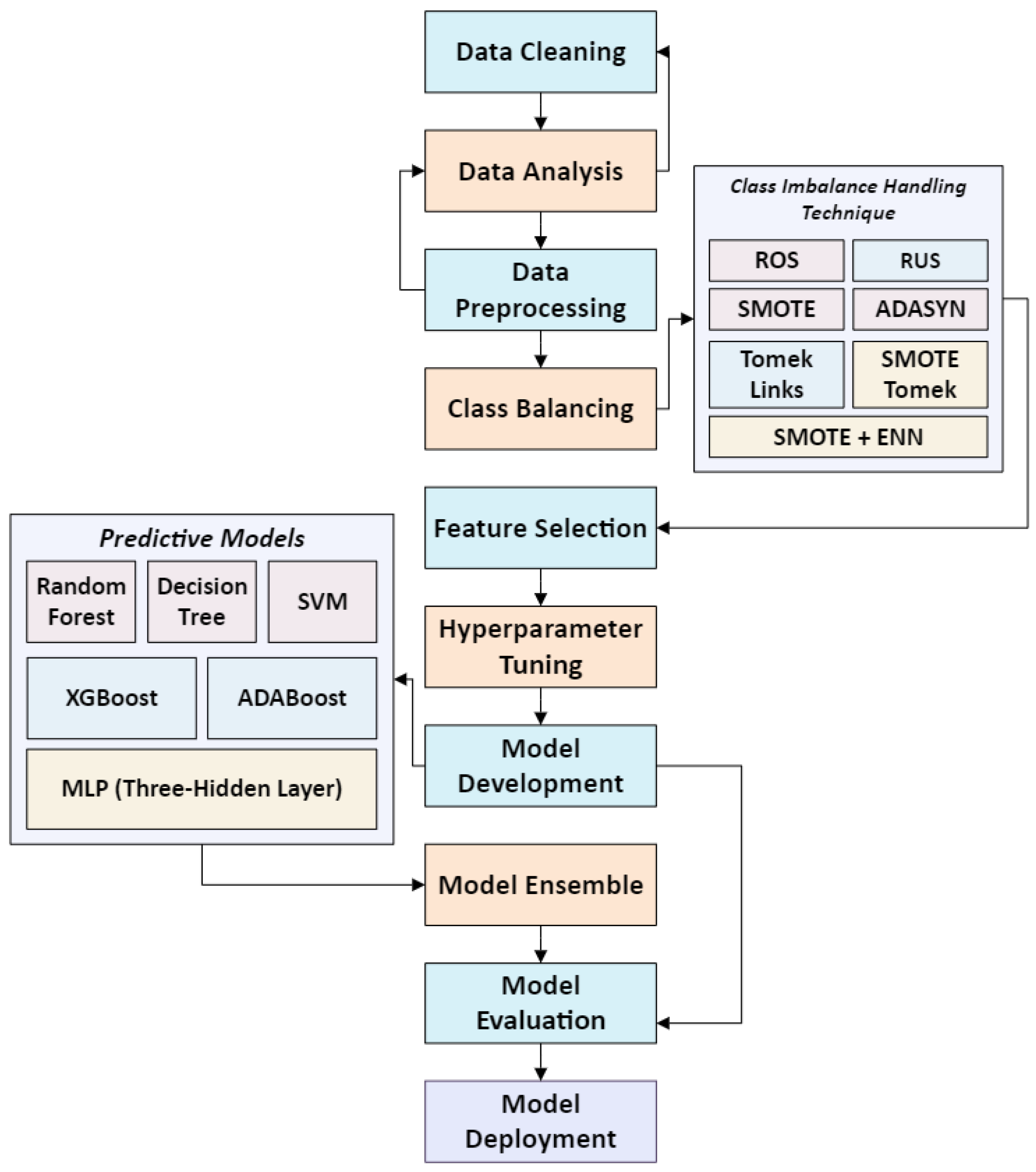
The framework of our approach illustrated in Figure 1, consists of different stages, where diverse techniques were tested (when required) to identify the most effective approach. The process is sequential, which means that each stage must be completed before the next stage begins. The subsequent sections outline the data preparation and analysis stages.

3.1. Data Cleaning

The next stage involved data cleaning and preprocessing, which prepared the data for proper analysis, ensuring the quality and reliability of the data. The approach used was similar to [17], which involved performing multi-observation cleaning such as handling missing values, identifying and correcting errors or inconsistencies and removing features that could potentially bias the analysis. The dataset contained no duplicates, however, there were 104 features with missing values. The columns with more than 50% of their data missing were excluded from the analysis. Additionally, categorical features with large number of missing values that were deemed as not useful for the analysis were removed, ‘emp_title’ with 142,402 unique values, ‘title’ with 21,976 unique values that were similar to ‘purpose’ feature and ‘emp_length’ which showed similar bad loan rates (%) across its group, were removed. Moreover, to avoid losing vital information from the numerical columns, the strategy to handle the missing values was derived based on the distribution (skewness and kurtosis), SciPy was used in calculating the Fisher-Pearson coefficient:

$$\mathrm{Skewness}={\displaystyle \frac{{\mathrm{m}}_3}{{{\mathrm{m}}_2}^{3/2}}}$$

(2)

where,

$i$th central point ($m_i)$is defined as:

$${\mathrm{m}}_{\mathrm{i}}={\displaystyle \frac{1}{\mathrm{N}}}{\sum _{\mathrm{n}=1}^{\mathrm{N}}(\mathrm{x}\left[\mathrm{n}\right]-\stackrel{\mathrm{-}}{\mathrm{x}})}^{\mathrm{i}}$$

(3)

N = sample size

$\stackrel{\mathrm{-}}{\mathrm{x}}$ = mean

Median imputation which is robust to outliers was used for skewed features while mode imputation was carried out on features that were multimodal [27,28], to preserve data integrity.

Pearson correlation coefficient $(\mathrm{r})$ is a filter method that measures the relationship between variables [29], and consistent with the approach used by [1], variables above 90% $\mathrm{r}$ with other features were removed, as they could cause multicollinearity, which may mislead the model’s performance [30]. It can be calculated as:

$$\mathrm{Correlation}\left(\mathrm{r}\right)={\displaystyle \frac{\sum ({\mathrm{x}}_{\mathrm{i}}-\stackrel{\mathrm{-}}{\mathrm{x}}\left)\right({\mathrm{y}}_{\mathrm{i}}-\stackrel{\mathrm{-}}{\mathrm{y}})}{\sqrt{\sum {({\mathrm{x}}_{\mathrm{i}}-\stackrel{\mathrm{-}}{\mathrm{x}})}^2\sum {({\mathrm{y}}_{\mathrm{i}}-\stackrel{\mathrm{-}}{\mathrm{y}})}^2}}}$$

(4)

3.2. Data Analysis

Descriptive analysis, such as count, mean, median, and standard deviation were used to summarise the numerical features and identify errors, furthermore, data visualisation was used to analyse the features and remove the ones that do not add any information. Which allowed some features to be excluded, and the state information ‘addr_state’ to be converted to region, so as not to completely miss out on any benefit that the location might have. Additionally, the descriptive analysis showed that there were outliers and possible errors in some features, for instance, ‘annual_inc’ had a maximum value of $9,522,972, which is a possible error, which would likely affect the debt-to-income ratio ‘dti’, which showed a maximum DTI of 999.00%. The errors and outliers were handled in the data pre-processing stage.

Table 1. Descriptive Analysis of Annual Income and DTI.

Features	count	mean	std	50%	max
annual_inc	403,593	76,278.3	71,140.2	65,000	9,522,972
dti	403,593	18.26	10.38	17.62	999

Table 1. Descriptive Analysis of Annual Income and DTI.

Features	count	mean	std	50%	max
annual_inc	403,593	76,278.3	71,140.2	65,000	9,522,972
dti	403,593	18.26	10.38	17.62	999

3.3. Data Pre-Processing

This stage is very important in getting the data ready for model development, here, observed errors are removed, outliers are treated, features are binned and combined to capture more information, categorical data are one-hot encoded and transformed to numerical data, finally, the values are normalised [31,32]. At each stage different techniques were tested, using XGBoost, to identify the best technique to utilise, similar to [10]. This model was selected because it is simple yet powerful and is known for its ability to generalise well to other models, moreover, they are efficient, which helped to save time [33], this approach was done to improve the performance of the models. Furthermore, after the observed errors in features like ‘annual_inc’ and ‘dti’ were removed, and categorical features shown in Table 2 were one-hot encoded, the outliers observed in the numerical features were handled, and the data was normalised.

3.3.1. Handling Outliers

Outliers are extreme values that are different from the rest of the data, and can influence some models, which is why it needs to be addressed. The best technique to handle the outliers was identified to reduce the effect of the outliers while retaining as much data as possible. The below methods were tested:

Standard score (z-score): Informs on how far a data value (V) deviates from the mean ($\mu )$, in regard to the standard deviation ($\sigma$). Z-score (Z) greater than 3 shows the extreme values, and is calculated as:

$$Z={\displaystyle \frac{(\mathrm{V}-\mathsf{\mu })}{\mathsf{\sigma }}}$$

(5)

Interquartile Range (IQR): Q1 (first quartile: 25%) and Q3 (third quartile: 75%) were used for the calculation, and values that fall outside these bounds are considered outliers.

Clip: Considers the values below and above the 1st and 99th quartile as outliers.

Winsorize: Limits the extreme values to a specified percentile.

3.3.2. Data Normalisation

Features in a dataset with different range can affect some models, this was handled by scaling the features using the following normalisation techniques:

Standard scaler: Scales the new value (n) to follow a normal distribution, however, it can be affected by outliers. It is calculated as:

$$\mathrm{n}={\displaystyle \frac{{\mathrm{n}}_{\mathrm{i}}-{\mathrm{n}}_{\mathrm{mean}}}{\mathsf{\sigma }}}$$

(6)

Min-max scaler: Scales the data to [0,1] range. Although it is not as sensitive to outliers as the standard scaler, it however can be influenced by them. It is calculated as:

$$\mathrm{n}={\displaystyle \frac{\mathrm{n}-\mathrm{minimum}\left(\mathrm{n}\right)}{\mathrm{maximum}\left(\mathrm{n}\right)-\mathrm{minimum}\left(\mathrm{n}\right)}}$$

(7)

Robust scaler: Uses median and IQR which reduces the effect of outliers. It is calculated as:

$$\mathrm{n}={\displaystyle \frac{{\mathrm{n}}_{\mathrm{i}}-{\mathrm{n}}_{\mathrm{median}}}{\mathrm{IQR}}}$$

(8)

3.3.3. Evaluation Metrics

To assess the effectiveness of the models including the model used in testing (XGBoost), various metrics were used. Additionally, they were used in this stage to identify the best pre-processing techniques to use.

Accuracy which measures the ratio of the correct predictions (both “positive” defaults and “negative” non-defaults) to the total number of predictions:

$$\mathrm{Accuracy}={\displaystyle \frac{\mathrm{TP}+\mathrm{TN}}{\mathrm{TP}+\mathrm{TN}+\mathrm{FT}+\mathrm{FN}}}$$

(9)

Precision which measures the proportion of the actual defaults among all default predictions:

$$\mathrm{Precision}={\displaystyle \frac{\mathrm{TP}}{\mathrm{TP}+\mathrm{FP}}}$$

(10)

Recall which is also known as sensitivity or True Positive Rate (TPR), measures the proportion of the actual defaults that are correctly identified, calculated as:

$$\mathrm{Recall}\left(\mathrm{Sensitivity}\right)={\displaystyle \frac{\mathrm{TP}}{\mathrm{TP}+\mathrm{FN}}}$$

(10)

AUC which measures the ability of the model to differentiate between defaulters and non-defaulters across all classification thresholds and is particularly useful in an imbalanced dataset. ROC curve plots the TPR against the False Positive Rate (FRP).

3.3.4. Identifying Data Pre-Processing Techniques

Recall, precision, and accuracy are metrics used in the selection process. The result can be seen in Table A1. The ‘winsorize’ method was identified as the technique to use in handling the outliers, and the ‘robust scaler’ was used for the data normalisation.

3.4. Addressing Class Imbalance

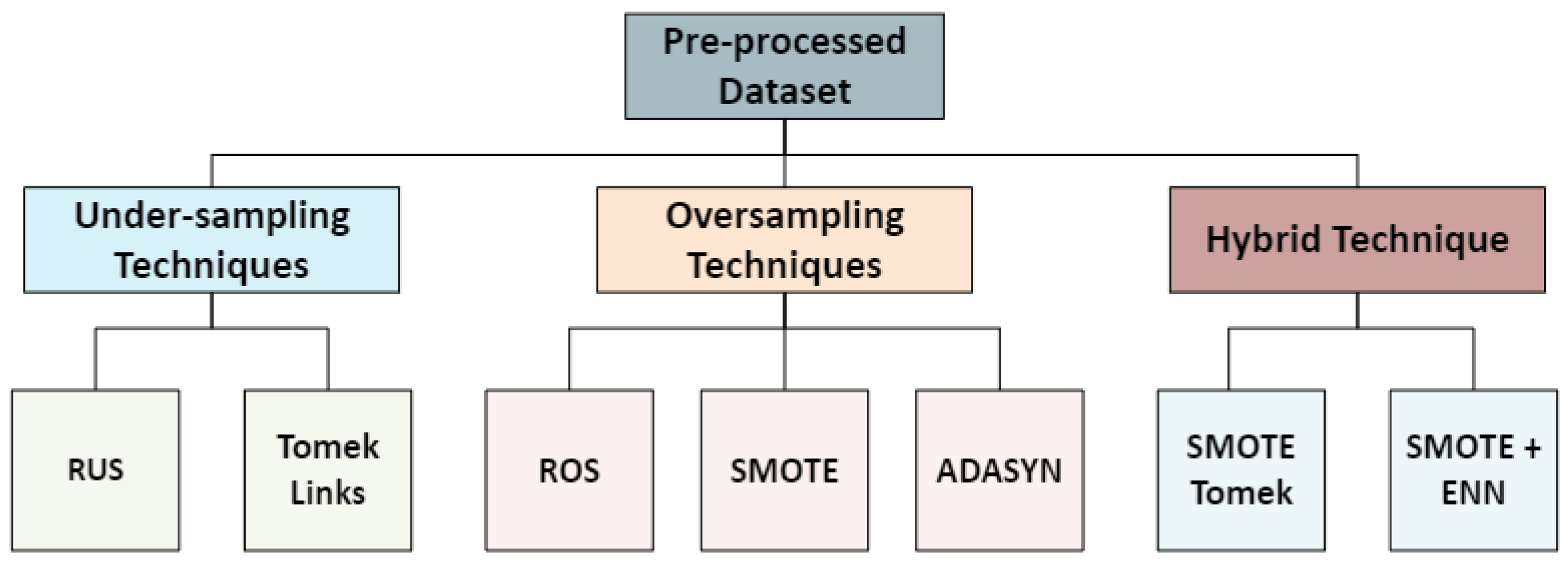
There are several techniques that can be used to tackle the issue of class imbalance, but no single one is regarded as the best. While popular techniques like SMOTE and ADASYN are used frequently, this research requires that the best technique to make use of is identified, therefore, different techniques were tested as shown below:

Figure 2. Class Imbalance Handling Techniques.

Figure 2. Class Imbalance Handling Techniques.

The techniques evaluated are:

Random Over-Sampling (ROS): It works by randomly adding data samples from the minority class to the dataset until the whole data is balanced [33,34]. It can be represented as

$$\mathrm{New}{\mathrm{S}}_{\mathrm{minority}}={\mathrm{S}}_{\mathrm{minority}}\cup \text{{}{\mathrm{S}}_{\mathrm{minority}}\mathrm{duplicated}\mathrm{until}\left|{\mathrm{S}}_{\mathrm{minority}}\right|={\mathrm{N}}_{\mathrm{majority}}\text{}}$$

(11)

where,

${\mathrm{S}}_{\mathrm{minority}}$ = minority class samples.

${\mathrm{N}}_{\mathrm{majority}}$ = Number of majority class samples.

$\left|{\mathrm{S}}_{\mathrm{minority}}\right|$ = Current size of the minority class.

Random Under-Sampling (RUS): It works by filling the minority class with data from the majority class, thereby reducing the majority class until the whole data is balance [34]. It can be shown as:

$$\mathrm{New}{\mathrm{S}}_{\mathrm{majority}}={\mathrm{S}}_{\mathrm{minority}}\cup \text{{}{\mathrm{S}}_{\mathrm{majority}}\mathrm{duplicated}\mathrm{until}\left|{\mathrm{S}}_{\mathrm{majority}}\right|={\mathrm{N}}_{\mathrm{minority}}\text{}}$$

(12)

SMOTE: It works by generating synthetic data through interpolating between the existing minority class data samples and their nearest neighbour, thereby adding new data point without adding duplicates [9,36]. It generates synthetic data (${\mathrm{x}}_{\mathrm{new}})$with:

$${\mathrm{x}}_{\mathrm{new}}={\mathrm{x}}_{\mathrm{i}}+\text{⋋}*({\mathrm{x}}_{\mathrm{nn}}-{\mathrm{x}}_{\mathrm{i}})$$

(13)

where,

${\mathrm{x}}_{\mathrm{i}}$ = minority class.

${\mathrm{x}}_{\mathrm{nn}}$= one of the nearest neighbours.

$\text{⋋}$ = a random value between [0, 1].

ADASYN: It works in a similar way to SMOTE, but it focuses on generating more synthetic samples for the harder to classify minority class, the number of the synthetic sampled $\mathrm{i}$, $\left({\mathrm{G}}_{\mathrm{i}}\right)$ is calculated as:

$${\mathrm{G}}_{\mathrm{i}}={\mathrm{d}}_{\mathrm{i}}*\mathrm{G}$$

(14)

where,

${\mathrm{d}}_{\mathrm{i}}$ = ratio of the majority neighbours.

$\mathrm{G}$ = total synthetic samples needed.

Tomek-Links is an under-sampling technique that cleans up the data by locating and removing ambiguous or noisy data samples that are near the decision boundary [36,37]. Given a majority class (${\mathrm{x}}_1)$ and a minority class (${\mathrm{x}}_2)$, if they are the nearest neighbours and they belong to different classes, they form a Tomek Link and removing them will help to clean the boundary between classes.

SMOTE-Tomek: It is a combination of SMOTE and Tomek Links, firstly, SMOTE is used to generate the synthetic data samples for the minority class, then Tomek Links are removed to clean up the boundaries between classes, thereby improving the quality of the synthetic data [38].

SMOTE+ENN: It is a hybrid technique that improves the quality of the synthetic data created by SMOTE, as Edited Nearest Neighbour (ENN) is used to remove instances of misclassification of the nearest neighbour [35,36,37,38,39,40].

To address the issue of class imbalance in the LendingClub dataset, the resampling techniques were tested using XGBoost and evaluated using accuracy, precision, recall and AUC. After the data has been balanced, the next step involved testing various splits to determine the best split to use, with 20%, 25%, 30%, 35% and 40% test ratios evaluated. Subsequently, the selected split 80:20 was used in selecting the appropriate features for the model development in the next stage.

3.5. Feature Selection

Feature selection is a crucial step in model development, and the goal here is to get features that can be used to simple and efficient models, as deploying a model with large number of features can be computationally expensive, therefore, this stage facilitates the reduction and removal of redundant features that may not be useful for model development [9,22]. The primary method used in this stage was the wrapper feature selection method, Recursive Feature Elimination with Cross-Validation (RFECV), which is a method that iteratively uses learning algorithms to select the best features to make use of by evaluating the performance of the model [41]. This method aims to find the features that gives the best performance using a scoring metric (scorer) and given that the focus is to correctly predict defaults, recall was used. Additionally, the ‘step’ parameter was set to 1, which indicates that one feature is removed per iteration, moreover, redundant features were also removed, thereby ensuring that the best features are selected for the model development process.

3.6. Model Development Process

This process involved using the selected features in the development of predictive models, so as to identify the best performing model that can be used to identify credit default risk. Additionally, methods like hyperparameter tuning and ensemble methods are further used to optimise the models.

3.6.1. Predictive Models

Decision Tree, which has a tree structure that works by recursively splitting the data into subsets of the tree based on a decision rule [1]. It selects the best feature to split based on criteria like Gini index – the impurity of a node and the values closer to 0 are the purer nodes, it is calculated and is calculated as:

$$\mathrm{Gini}=1-\sum _{\mathrm{i}=1}^{\mathrm{c}}{(\mathrm{p}}_{\mathrm{i}}{)}^2$$

(15)

where,

${\mathrm{p}}_{\mathrm{i}}$ = proportion of the data sample that belongs to the class $i$ in a tree node.

$\mathrm{c}$ = number of classes.

Random Forest, an ensemble learning method that combines the predictions gotten from training multiple decision trees to get the final predictions [37,42]. The final predictions are made using majority voting. Since it is a combination of decision trees, it uses the Gini as well for splitting.

SVM, finds the optimal hyperplane that separates the data into different classes [23]. It uses kernel functions to handle non-linear separation by mapping input features into high-dimensional spaces. The hyperplane:

$$\mathrm{h}({\mathrm{x}\text{}}_{\mathrm{i}})=\mathrm{sign}(\mathrm{w}\text{⋅}{\mathrm{x}}_{\mathrm{i}}\text{}+\mathrm{b})$$

(16)

XGBoost, builds an ensemble of weak learners in an iterative manner in order to improve on the models’ performance [17]. It uses gradient boosting with specific loss functions $l$ and regularisation terms $\mathsf{\Omega }\left(f\right)$:

$${\mathrm{L}}^{\left(\mathrm{t}\right)}=\sum _{\mathrm{i}=1}^{\mathrm{n}}\mathrm{l}\left({\mathrm{y}}_{\mathrm{i}},{{\widehat{\mathrm{y}}}_{\mathrm{i}}}^{\left(\mathrm{t}-1\right)}+{\mathrm{f}}_{\mathrm{t}}\left({\mathrm{X}}_{\mathrm{i}}\right)\right)+\mathsf{\Omega }\left({\mathrm{f}}_{\mathrm{t}}\right)$$

(17)

where,

$L^{\left(t\right)}$ = total loss at iteration $t$.

$n$ = data points.

$l\left(y_i,{{\widehat{y}}_i}^{\left(t-1\right)}+f_t\left(X_i\right)\right)$ represents the loss function that measures the difference between the true and predicted labels.

${{\widehat{y}}_i}^{\left(t-1\right)}$ is the previous iteration’s predicted class.

$f_t\left(X_i\right)$, is the current model’s prediction.

ADABoost, focuses on creating strong classifiers by combining multiple weak classifiers [43]. It trains weaker learners on the errors made by the previous ones, and when there is a misclassification, it assigns more weight to them. Final predictions are calculated by:

$$\mathrm{H}\left(\mathrm{x}\right)=\mathrm{sign}\left[\sum _{\mathrm{t}=1}^{\mathrm{T}}{\mathsf{\alpha }}_{\mathrm{t}}{\mathrm{h}}_{\mathrm{t}}\left(\mathrm{x}\right)\right]$$

(18)

where,

$T$ = weak classifiers.

${\alpha }_t$= weight for the weak classifier.

$h_t\left(x\right)$ = predictions for the weak classifier.

$sign$ = determines the final prediction

MLP, is a feedforward type of ANN that consist of the inner layer, multiple hidden layers and an outer layer, and each layer is made up of neurons connected to those in the previous and following layers. Each connection has a weight, and MLP uses backpropagation to adjust the weights based on the error in the output, and gradually increases the predictions. Furthermore, this model is capable of learning complex patterns in data.

3.6.2. Hyperparameter Tuning

This process can help in getting the best performance from each model, and similar to [41], GridSearchCv was used to get the parameters used for the model development. Some of the parameters used for GridSearchCV are shown in Table A2, the values were predominantly chosen to strike a balance between reducing overfitting and increasing the performance of the models, for instance, the max_depth limits the depth of the tree, therefore, the values chosen may capture complexity and make the model efficient. Additionally, for reg_alpha and reg_lambda, which are Lasso (L1) and Ridge (L2) regularisation terms, they allow XGBoost control sparsity as well as the magnitude of the model’s weights. The best parameters identified and used for the model development are shown in Table 3:

3.6.3. Ensemble Techniques

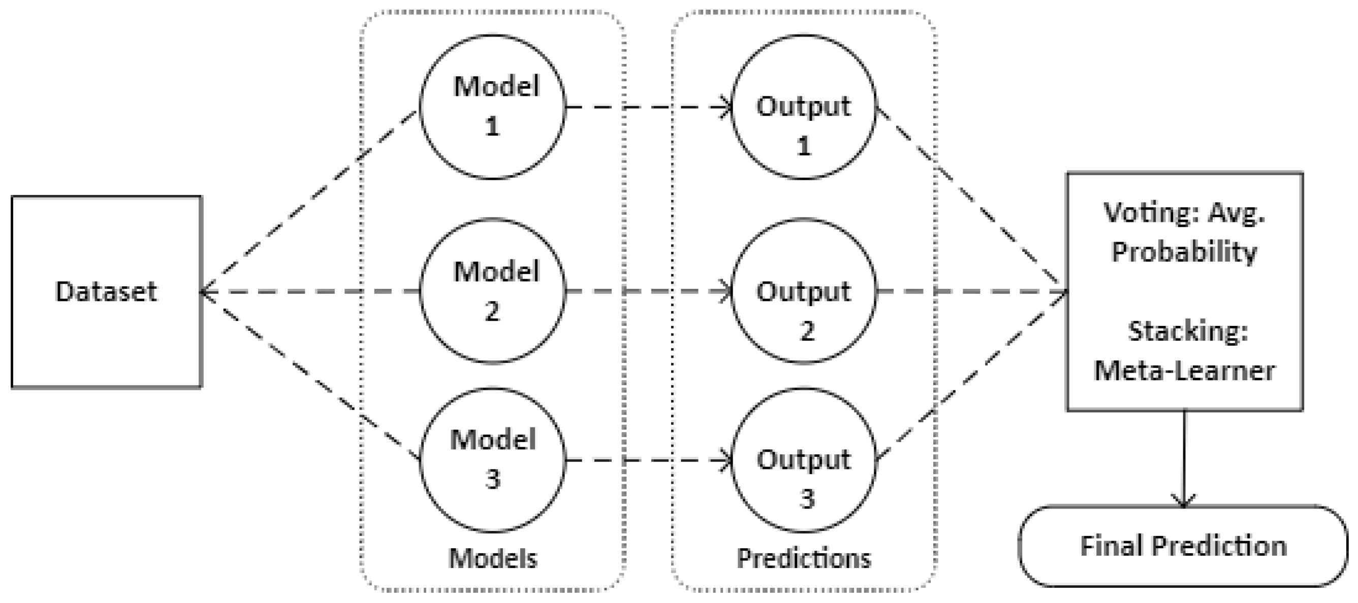
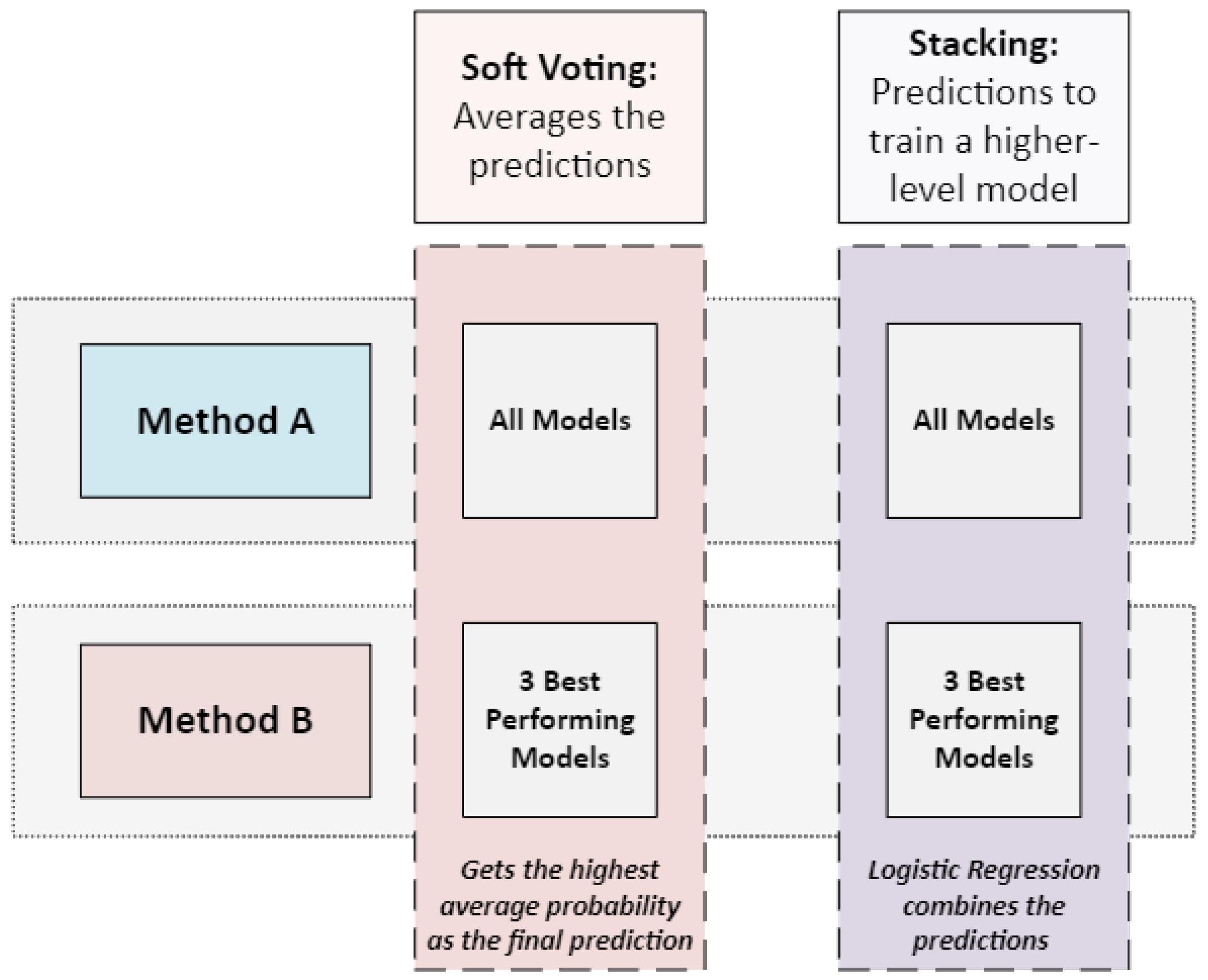
In this stage, some of the models, as well as the top three best performing models are combined using the voting and stacking method. The first method, soft voting, takes the average probability predictions from the models as the final prediction. Additionally, the second method uses the stacking method for the combination, here, a meta-model is used to get the final prediction, the meta-model learns how best to aggregate the predictions to make the final prediction. The ensemble methods used in this work and how they are combined is shown in Figure 3 and Figure 4 respectively.

Figure 3. Ensemble Methods.

Figure 3. Ensemble Methods.

Figure 4. Methods used in combining the model predictions.

Figure 4. Methods used in combining the model predictions.

4. Results

In this section, we present the results of the model development process discussed in Section 3.6. Additionally, we compare these results with those from other related studies, serving as a baseline to further validate the results obtained in this research. However, before we discuss the model performance, we first discuss the results related to addressing class imbalance and feature selection as outlined in Section 3.4 and Section 3.5. 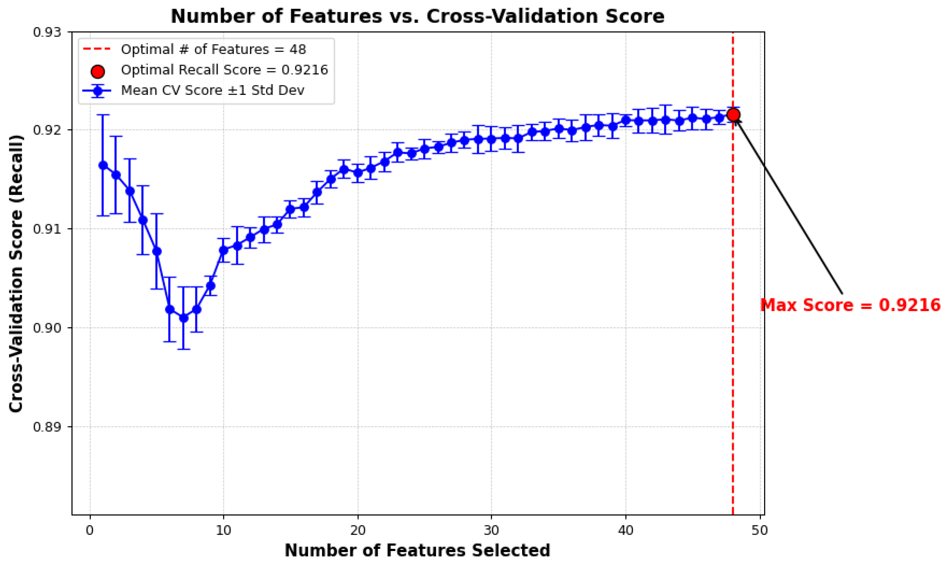Therefore, Table 4 shows the results of employing the sampling techniques, while Figure 5 shows the results from using RFECV.

As presented in Table 4, ROS performed better than RUS, which coincides with the observation made by [9], that the oversampling technique always performed better than the under-sampling technique, and while ADASYN, SMOTE and SMOTE-Tomek showed impressive results, SMOTE+ENN showed the most impressive performance across all the metrics, hence, by combining both SMOTE and ENN, the data is not only being balanced, the noise or ambiguous data samples that may affect the model’s performance are also being removed [40]. Additionally, with a recall of 92.02%, it showed that the model captures the minority class correctly, which is sometimes more important than getting a high accuracy. Furthermore, given the result, SMOTE+ENN was used to balance the dataset.

Additionally, Figure 5 shows how the recall changes as the features are added, with the optimal features identified when the score plateaus, it also shows the standard deviation of the CV scores, which shows the variability and stability of the model’s performance across the folds, with 48 features identified as the optimal number of features to get the optimal recall score of 92.16%.

Figure 4. Features Selected.

Figure 4. Features Selected.

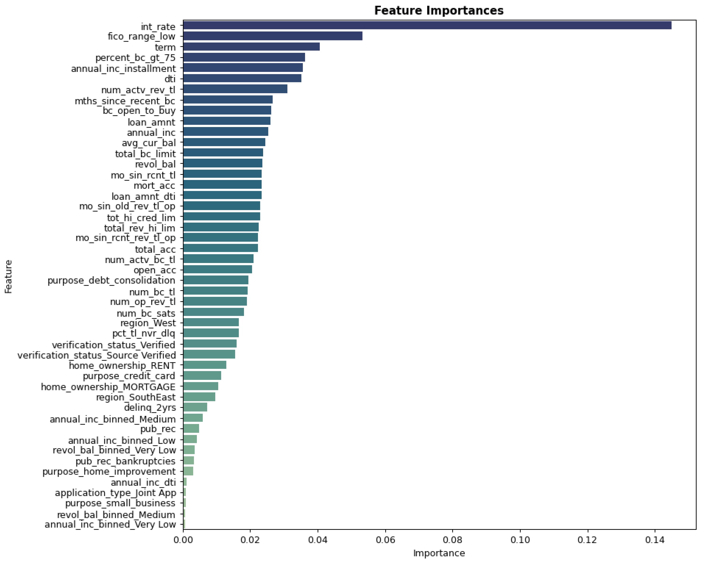
Additionally, the results for the feature importance are shown in Figure 5 below, with the interest rate, credit score and the loan term, identified as the most important features in the prediction of credit default. Based on these findings and the best parameters listed in Table 3 (Section 3.6.3), the models were subsequently developed.

Figure 5. Feature Importance.

Figure 5. Feature Importance.

4.1. Model Performance Evaluation

4.1.1. Individual Model Performance

The metrics discussed in Section 3.3.3 were used in the evaluation of the model performance, with the performance of the individual models presented in Table 5:

Table 5. Individual Model Result.

Model	Accuracy	Precision	Recall	AUC
Random Forest*	0.8987	0.8996	0.9656	0.9589
Decision Tree	0.7778	0.7743	0.9713	0.7256
SVM	0.7318	0.9476	0.6601	0.8824
XGBoost*	0.9156	0.9478	0.9330	0.9726
ADABoost	0.8458	0.8548	0.9439	0.9305
MLP*	0.8775	0.9008	0.9305	0.9229
*Indicates models part of the ensemble with 3 base-learners

Table 5. Individual Model Result.

Model	Accuracy	Precision	Recall	AUC
Random Forest*	0.8987	0.8996	0.9656	0.9589
Decision Tree	0.7778	0.7743	0.9713	0.7256
SVM	0.7318	0.9476	0.6601	0.8824
XGBoost*	0.9156	0.9478	0.9330	0.9726
ADABoost	0.8458	0.8548	0.9439	0.9305
MLP*	0.8775	0.9008	0.9305	0.9229
*Indicates models part of the ensemble with 3 base-learners

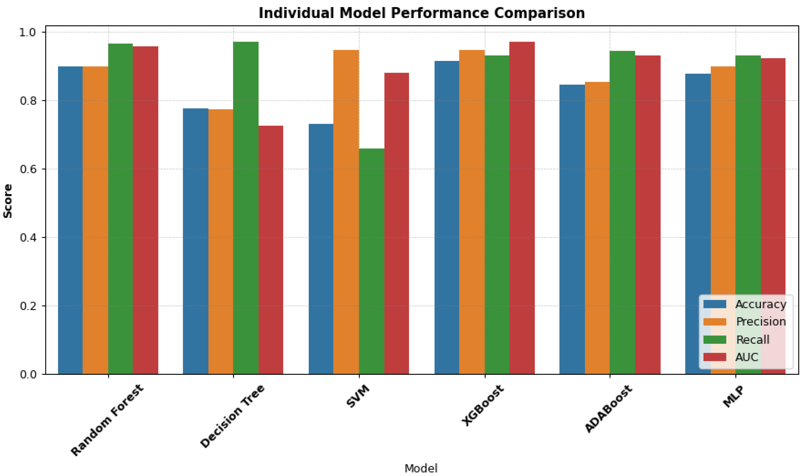
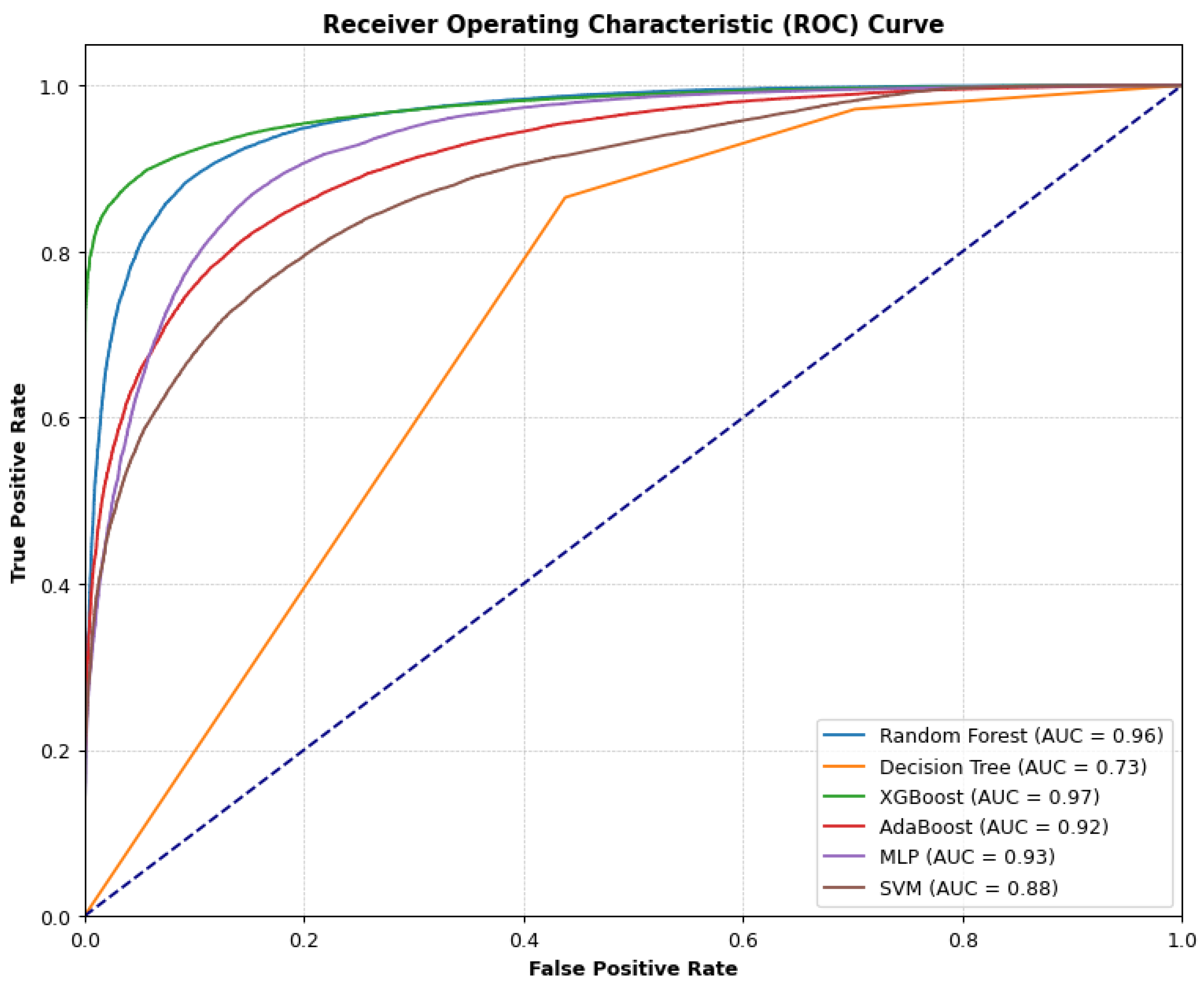
Models with ensembled techniques like Random Forest and XGBoost outperformed simpler models like Decision Tree and SVM, which shows the advantages of combining model predictions to improve their effectiveness. The models – Random Forest and XGBoost showed strong performances with an accuracy of 89.87% and 91.56% respectively. Additionally, the recall, which indicates that the models can effectively identify default cases are 96.56% (Random Forest) and 93.30% (XGBoost), with high AUC scores of 95.89% and 97.29%, which suggests that the models are able to effectively distinguish between the defaulters and the non-defaulters. Similarly, with a recall of 92.48%, MLP had a solid performance, however, SVM had the lowest score, despite having a high precision value of 94.76%, which may suggest that SVM is not able to address the complexity of the credit default data.

The ROC curve in Figure 6 shows the performance of the individual models across different thresholds, displaying how well the models separate the non-default and the default class, furthermore, it shows that all the models performed well.

For the individual models XGBoost with an accuracy of 91.56%, precision of 94.78% and AUC of 97.26% achieved the best results, which shows how effective the model is at handling complex credit default data, with the performance being attributed to XGBoost’s ability to create better predictions by combining the predictions from weaker learners, as well as the built-in regularisation that helps to prevent overfitting, giving it an edge, especially when compared to the other models:

Figure 7. Comparative Result (Individual Model).

Figure 7. Comparative Result (Individual Model).

4.1.2. Ensemble Model Performance

As detailed in Section 3.6.3, the predictions from the individuals can be combined to create stronger learners. The result of combining the models’ predictions is shown below:

Table 6. Ensemble Model Result.

Model	Accuracy	Precision	Recall	AUC
Voting A	0.9109	0.9099	0.9710	0.9703
Voting B	0.9166	0.9314	0.9532	0.9687
Stacking A	0.9369	0.9559	0.9555	0.9781
Stacking B	0.9188	0.9409	0.9454	0.9708

Table 6. Ensemble Model Result.

Model	Accuracy	Precision	Recall	AUC
Voting A	0.9109	0.9099	0.9710	0.9703
Voting B	0.9166	0.9314	0.9532	0.9687
Stacking A	0.9369	0.9559	0.9555	0.9781
Stacking B	0.9188	0.9409	0.9454	0.9708

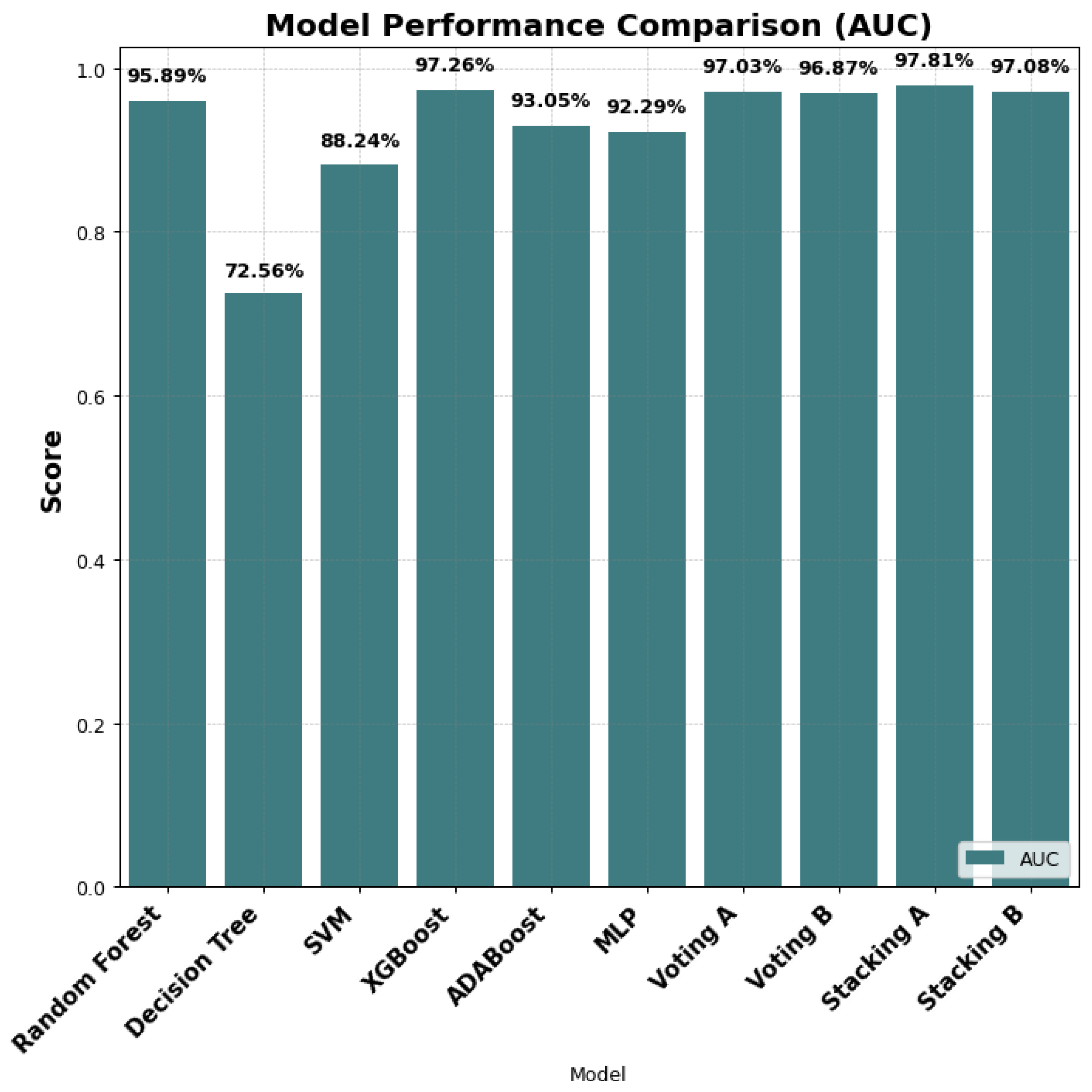
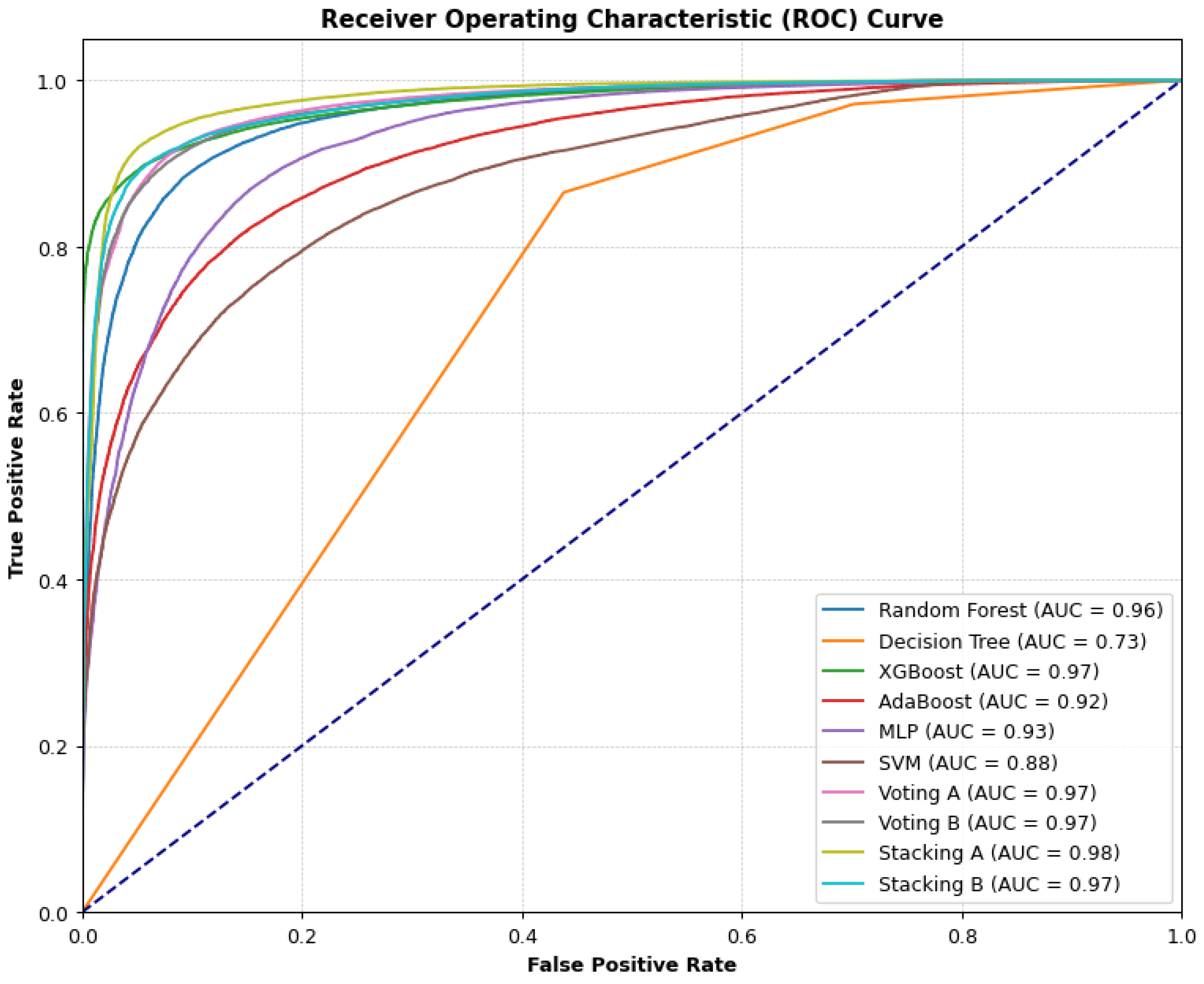
Combining the models led to an overall increase in the performance, especially when the predictions are combined with the ensemble model which uses a learner model (meta-model) – Stacking. The method A, which combines the predictions from all the models achieved the highest result overall (Staking A), with an accuracy of 93.69%, precision of 95.59 and AUC of 97.81%, which suggests that combining the models with the stacking technique led to an improvement in the performance.

Although XGBoost and the ensemble methods – Voting A, B and Stacking A, B performed well, as seen in Figure 8, however, Stacking A’s performance is impressive, as it is identified as the best model with the ability to effectively separate the classes. This demonstrates the need for the inclusion of more algorithms in the ensemble process, therefore, we propose this technique for the classification of credit default risk. Furthermore, with a precision and recall of approximately 96%, the model shows how well the technique can enhance the individual models, as it uses a meta-model to learn how best to combine predictions.

The comparative result can be seen below, with Stacking A outperforming the other models, with an AUC of 98%, thereby showing how effective ensemble methods can be at optimising the performance of the models.

Figure 9. Comparative Result (All Models).

Figure 9. Comparative Result (All Models).

4.2. Comparison with Baseline Results

The performance of the proposed model is compared with other related works, which served as the baseline for further evaluation. The result can be seen below:

Table 5. Baseline Comparison.

Reference	Dataset	Total Record	Model	Result
Proposed Method	LendingClub	394,073	Stacking	93.7%
[9]	Taiwan Credit-Client	30,000	GBDT*	88.7%
	South German Credit-Client	1,000		83.5%
	Belgium Credit-Client	285,299		86.3%
[10]	LendingClub	282,763	XGBoost	87.9%
[11]	Data from Kaggle (Chatterjee, 2021)	614	Voting	87.3%
[12]	Auto-Finance	25,383	Deep Learning-Optimised Stacking	92.7%
*Gradient Boosted Decision Tree (GBDT)

Table 5. Baseline Comparison.

Reference	Dataset	Total Record	Model	Result
Proposed Method	LendingClub	394,073	Stacking	93.7%
[9]	Taiwan Credit-Client	30,000	GBDT*	88.7%
	South German Credit-Client	1,000		83.5%
	Belgium Credit-Client	285,299		86.3%
[10]	LendingClub	282,763	XGBoost	87.9%
[11]	Data from Kaggle (Chatterjee, 2021)	614	Voting	87.3%
[12]	Auto-Finance	25,383	Deep Learning-Optimised Stacking	92.7%
*Gradient Boosted Decision Tree (GBDT)

The proposed method displays a higher accuracy when compared with the other results, [9] achieved accuracy scores ranging from 83.5% to 88.7% using GBDT, with results varying across the different datasets, additionally, [10] achieved an accuracy of 87.9% with the XGBoost model on LendingClub dataset, moreover, [12] achieved an accuracy of 92.7% with Deep Learning-Optimised Stacking, an ensemble model. However, the proposed result performed better with a score of 93.7%, showing how well the model is at predicting credit default.

Finally, SHAP (SHapley Additive exPlanations) with XGBoost model was used to analyse and explain the features as shown in Table A3, with the features resulting in negative values, contributing to the predictions being lower, thereby increasing the likelihood of defaults, for instance, a negative ‘int_rate’ means that higher interest rate pushes the prediction towards default, while positive values, contributes to the predictions being higher, for instance, positive ‘fico_range_low’ means that higher credit scores move the prediction away from being classed as a default. With the proposed model developed, tested and evaluated, this research shows how well the methodology used worked, as testing the techniques to identify the most suitable one contributed to the overall performance of the models, additionally, combining the predictions from wearker classifiers contributed as well.

5. Conclusion and Recommendations

In this study, various techniques have been explored to identify the best techniques to use, as well as to handle the issue of class imbalance. Additionally, diverse machine learning and deep learning models have been explored to predict the likelihood of loan default – Random Forest, Decision Tree, Support Vector Machine (SVM), Extreme Gradient Boosting (XGBoost), Adaptive Boosting (ADABoost) and Multi-Layered Perceptron (MLP) with three-hidden layer.

Voting and stacking ensemble techniques have been employed to optimise the models, with the stacking method combining the predictions from all the models identified as the best-performing model. The proposed model is capable of precisely gauging default risk, with a recall of 95.5%. Moreover, when comparing the results from this research with those from the baseline results as shown in Section 4.2, this study was able to achieve higher accuracy, 93.7%. Furthermore, this research can help with future work, as the performance of diverse techniques and models has been explored and documented.

The techniques and findings obtained from this research may create interesting avenues for future research, for instance, in the selection of suitable techniques to use, instead of using XGBoost as a test model, each technique can be tested on each model to see if different techniques work better with different models, additionally, the methodology can be tested on other credit datasets, to further validate the selected framework.