1. Introduction
According to Moore’s law, “the number of transistors that can be placed on a chip doubles every 24 months” [
1]. Maintaining Moore’s law is highly challenging, because it calls for continuous advancement in a very complex industry. Despite this, recent developments in the production of integrated circuits (ICs), particularly in photolithography, have enabled the industry to keep up with the high process standards. Owing to its role in transferring a desired pattern to a photosensitive material on the wafer surface (photocurable material; most frequently, commercial photo resist; [
2]) by exposing it to ultraviolet (UV) or Extreme-UV (EUV) light, photolithography [
3] is a crucial component of the entire process. Wafers with a high overlay (OVL) and small critical dimension (CD) are the result of a successful photolithography process. The smaller the exposed pattern and the smaller the exposed ICs on the wafer, the better the OVL and the smaller the CD. Therefore, photolithography is the most crucial step in the production of integrated circuits consisting the base mechanism that supports Moore’s law.
In terms of hardware and software, photolithography machines rank among the most complex machines in the market. It is highly challenging to orchestrate and operate the machine in such a way that it satisfies the extremely stringent OVL and CD standards given the machine’s more than 50 million lines of code and thousands of hardware modules. This precision is impossible for the hardware alone. Software control techniques that cope with hardware imperfections are essential components of the machine. Software will enable the machine to meet the OVL and CD KPIs, which will confirm the machine’s quality.
The fundamental premise underlying this is that the machine can precisely model anticipated wavefront aberrations at the nanoscale level. The software then adjusts the associated machine knobs, such as mirror locations, such that it compensates for the anticipated aberrations because it knows what to expect. The required pattern is then exposed to the fewest possible flaws because the predicted fingerprint is rectified before it reaches the wafer surface. Under these circumstances, we recognize that one of the most important and difficult responsibilities of the photolithography process is the ability to create precise models. These models are the primary tools for successful exposure.
The process of describing the spatial changes in the overlay (OVL) of the features being printed is known as OVL fingerprint estimation (FE) in photolithography. These discrepancies can be caused by several factors, including flaws in the mask or the lithography procedure itself. The OVL of the features at various positions on the wafer are often measured using specialized metrology instruments that can estimate fingerprints. Information regarding the spatial changes in the OVL is then extracted from the resulting data and utilized to generate a “fingerprint” of the lithography process. Modeling the OVL is an essential step in the FE process. OVL modeling is the process of creating mathematical and statistical models to forecast how various process parameters affect OVL. By modifying the lithography process parameters in real time to meet the necessary OVL criteria, these models can be used to improve the lithography process. To ensure a high yield and reliable performance of the lithography process, FE estimation is a crucial tool.
A polynomial model is a mathematical or statistical representation of a system or process and polynomial. The basis functions and parameters are the two main components of the model. The structure of the problem and the properties of the data being modeled influence the basis functions that are used. On the other hand, model parameters are the estimated values that are used to define the model and are derived from the data. The precise values of the basis functions that best suit the data are determined by the parameters. In our specific use case, we need to provide the model for OVL. A linear model for OVL is defined by:
is the information matrix which consists of the basis function
and
p are the parameters of our model. The OVL polynomial has P coefficients or parameters. As described above, the information matrix
is already known to us and in that case the goal of FE is to estimate the parameters
p of our model.
Overlay control is a critical part that enables the exposure system to successfully imprint the complex patterns and meet the strict requirements of modern IC designs. The current photolithographic systems manage to successfully control overlay via a combination of advanced process control (APC) and metrology modules. Metrology contributes into defining and tuning of the overlay models (so that they accurately describe the expected systematic and non-systematic overlay errors [
7,
8,
9]), as well as relating them to the corresponding controllable knobs of the exposure system [
10]. The coupling of overlay error predictions, via overlay models, with machine knobs defines the so called run-to-run (R2R) paradigm of overlay control [
11,
12,
13]. Obviously, for a R2R process to be successful it is crucial that the overlay models can accurately estimate the expected overlay errors. Extensive research has been conducted in defining overlay models. In [
14] multilevel state space models are defined based on existing physics models [
15,
16,
17] where multilayer, stack up overlay error models are developed. Extensive literature has been conducted for improving overlay modeling process with the focus being either on optimizing the wafer measurements ([
18,
19]) or in investigating different metrics and cost functions ([
20] Zhang
et al.)
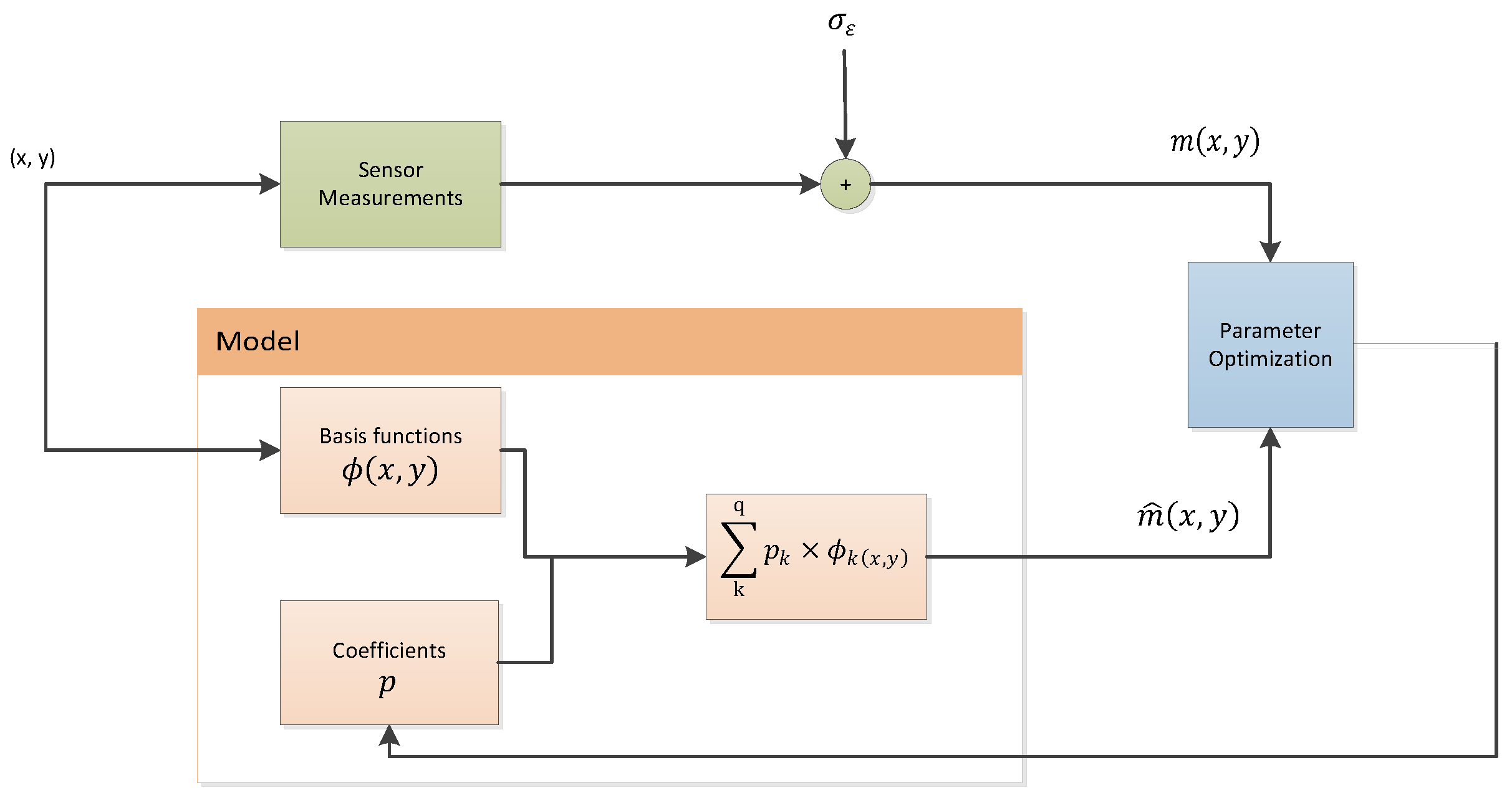
However, it is not sufficient to define the overlay model based only on the underlying physics; it is equally important that the metrology system further tunes the parameters of the overlay model. The Ordinary Least Squares optimization (OLS) method is the most employed regression technique by the current exposure systems. OLS finds the regression coefficients of the overlay model that minimize the residual sum of the squared errors of the difference between the measured and the predicted overlay [
21]. In
Figure 1, the process of FE is presented. Since the basis functions of the model
are already predefined, the goal of the FE process is to obtain the best estimation of the model parameters
p.
So far, this aspect of the problem, regarding the fitness of the OLS algorithm to model highly dimensional overlay data has not been extensively researched. In this paper we are investigating and proposing the usage of Ridge Regression over the classical OLS algorithm. The remainder of the paper is organized as follows: Section II describes the proposed method and in Section III we show the results of applying the proposed method on an actual industrial process of a 300mm wafers. Finally, Section IV presents the conclusions and potential future work.
2. Materials & Methods
In this paper we are proposing to use Ridge Regression instead of the classic OLS method for tuning the parameters
p of the overlay models. The overlay models as mentioned above consist of a set of basis functions
that are already predefined based on the physics and specific parameters of the process. Ridge regression or Tikhonov regularization [
22] is a statistical method for estimating the parameters of multiple regression models in scenarios where the independent variables are highly correlated.
Ridge regression is particularly useful in ill-posed problems which exhibit multicollinearity in their independent variables. In our case we try to find the vector
p of parameters such that:
As mentioned before the standard approach is to use the OLS method. OLS seeks to minimize the the sum of the squared residuals:
However if no p satisfies the equation or more p do, then the problem is ill-posed and OLS might lead to over- or under-determined system of equations.
Ridge regression adds a regularization term
for some suitable chosen matrix
. This is known as
regularization. This ensures smoothness and improves the conditioning of the problem. The minimization problem to be solved then is:
And the corresponding parameter vector
p:
In our proposal we are using which means that .
In
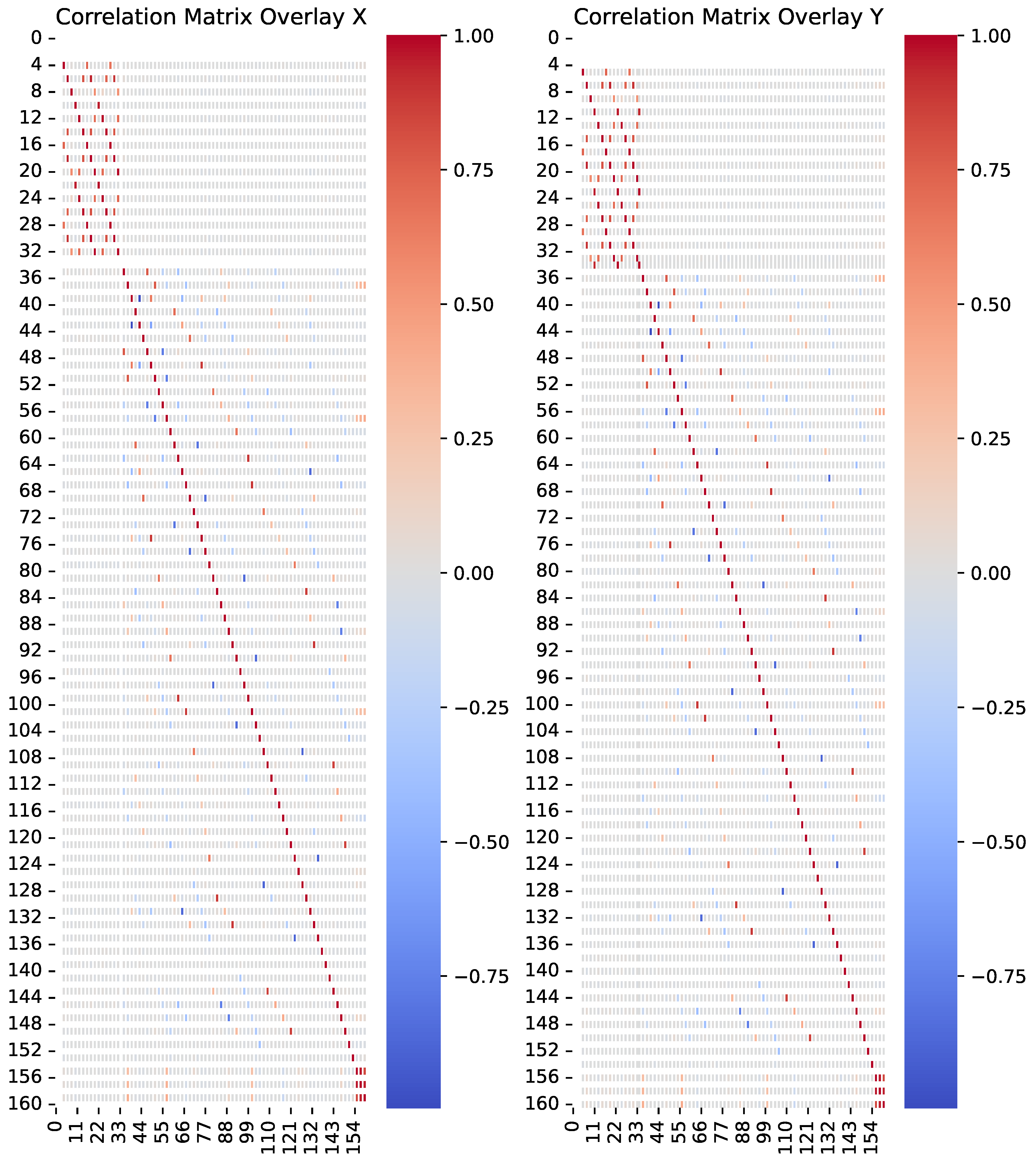
Figure 2 the Corelation Matrix of the Overlay X and Overlay Y is presented. There seems to be high correlation between approximately 50 of the 161 parameters. This is an indication (a strong one though) that there is significant collinearity in the parameters and this needs to be further investigated.
The Variance Inflation Factor (VIF) is a statistical measure that quantifies the degree of multicollinearity for each independent variable. VIF is calculated as:
with
being the square of the OLS solutions. A value of VIF > 5 indicates moderate multicollinearity while VIF > 10 indicated high multicollinearity. Performing the VIF check in our OLS solutions for Overlay X and Y results in high mulitcollinearity in 62/161 parameters for Overlay X and in 109/161 parameters for Overlay Y. So, the conclusion is that multicollinearity needs to be addressed. In this case, indeed the Ridge Regression method should be able to address the issue and improve the parameter estimation method.
3. Results & Discussion
In our experiments we compared the overlay residuals (in X and in Y) for both Ridge Regression and OLS methods. The expected overlay, per field point, is compared to the actual overlay and next a statistical analysis of the results is performed. In assessing the performance we are using the percentile and residual metrics. Utilizing these metrics enables a comprehensive understanding of the overlay performance, providing insights into the extent of variability and the upper bounds of error dispersion.
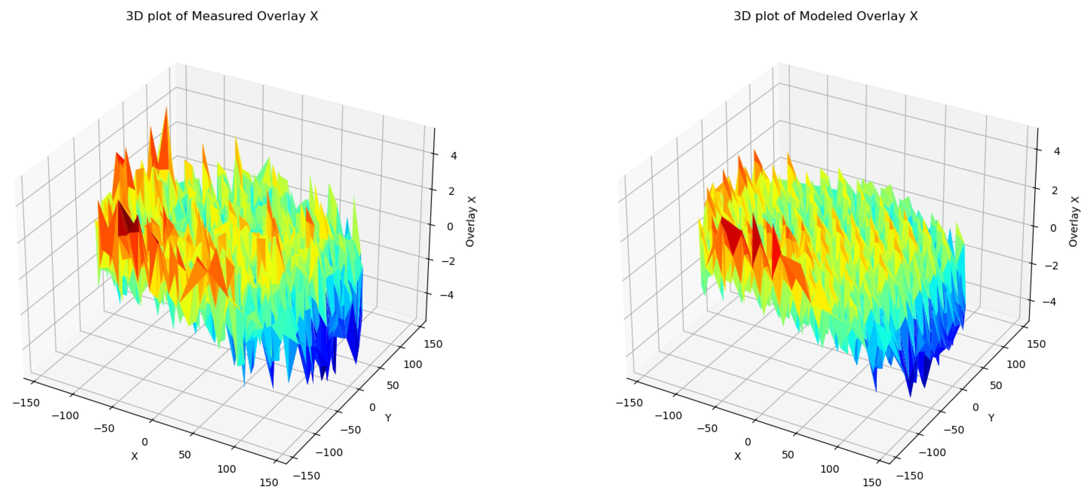
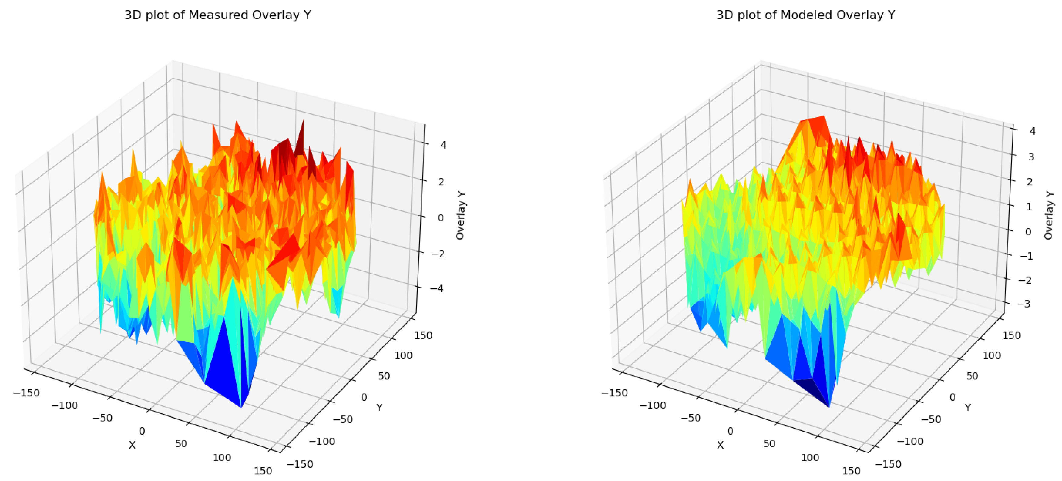
The goal of our method is to accurately model the measured overlay and reproduce it with minimum error. In
Figure 3 we can see the measured Overlay X on the left and the modeled Overlay X on the right, using the Ridge Regression Method. In this visual representation we can see that the modeled Overlay is able to capture successfully the expected overlay. Also in areas of the wafer where there seems to be abnormal behavior as on the edges of the wafer, the patterns seems to really match. Similarly in
Figure 4, Ridge Regression also performs well on the Overlay Y.
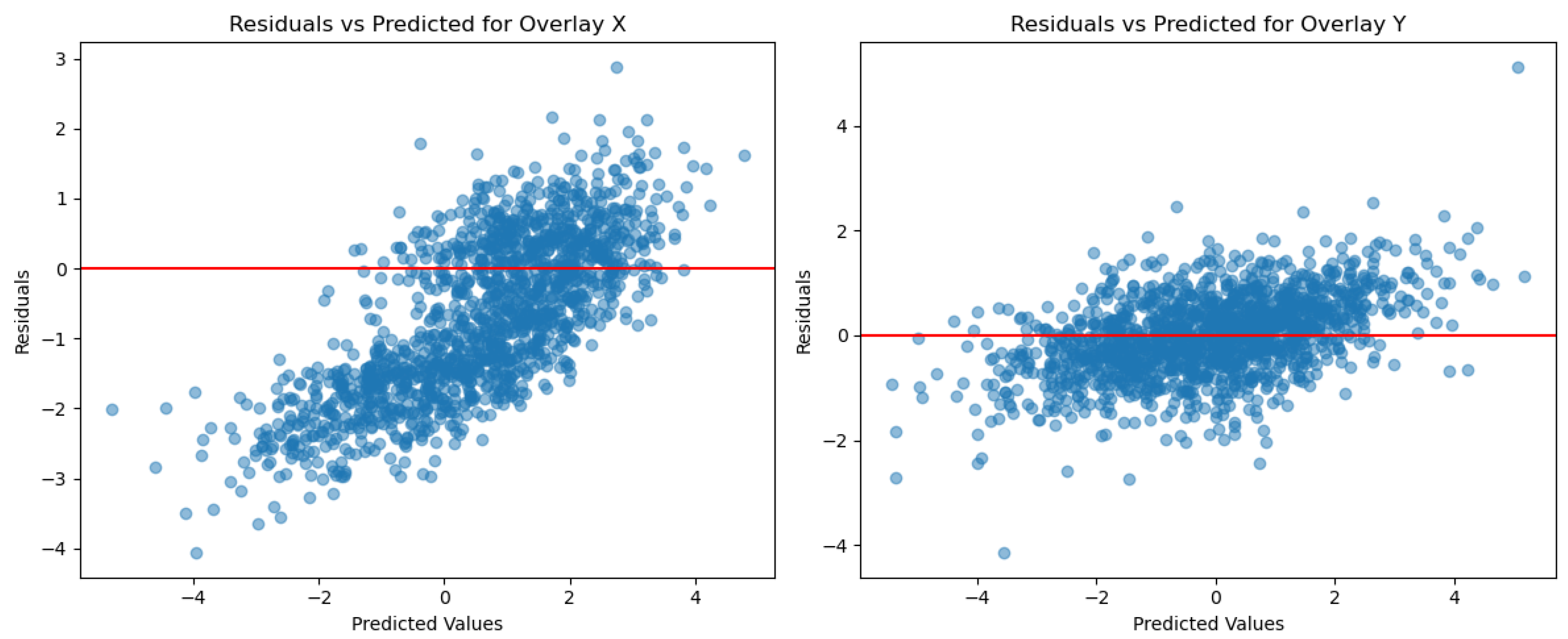
The resisuals vs. the predicted values for Overlay X and Y are presented in
Figure 5 too.
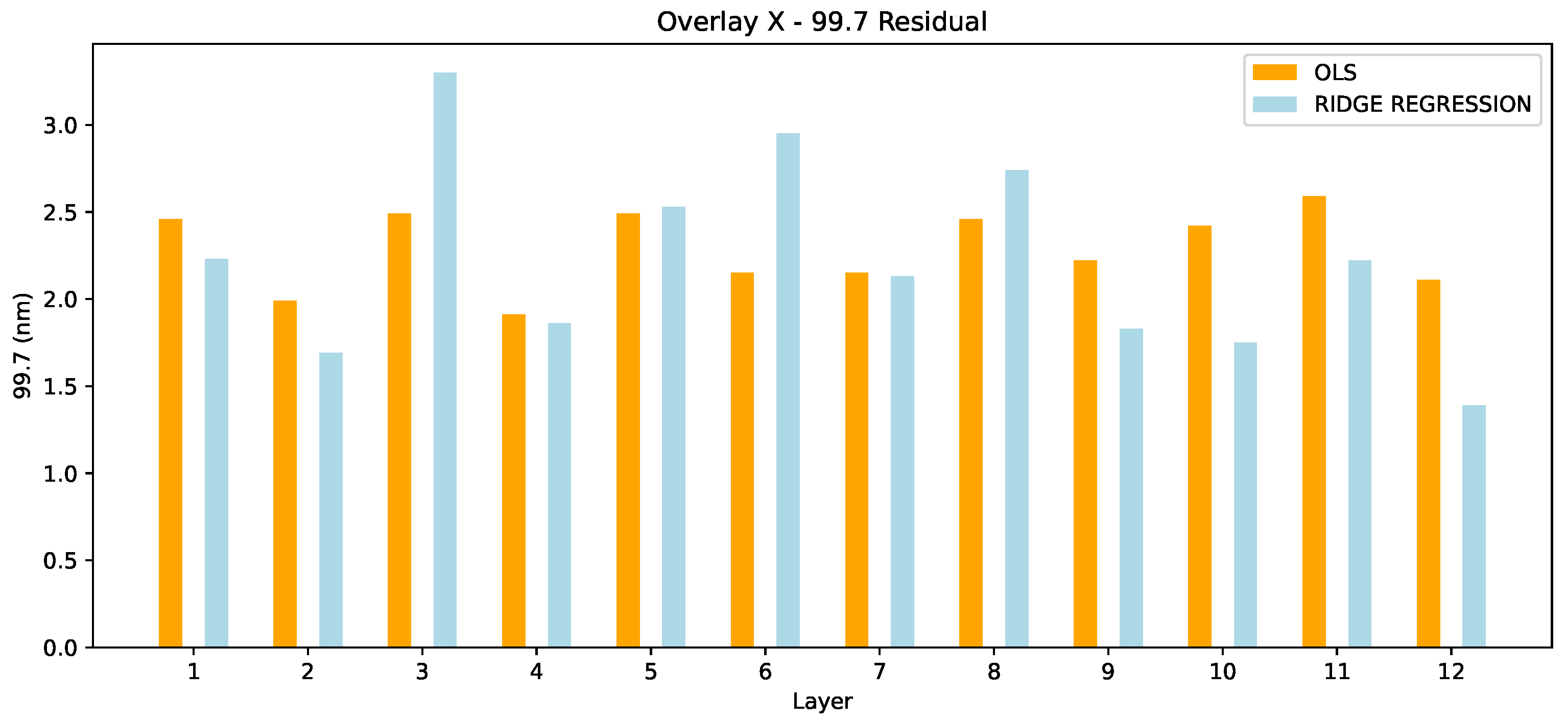
In
Figure 6 the Overlay X residuals in 99.7 are presented, for both OLS and Ridge Regression methods. For 8/12 layers ridge regression outperforms OLS method. OLS still is better than Ridge Regression in layers 3, 5, 6 but given the notably high residuals in Ridge Regression we can consider these results as outliers.
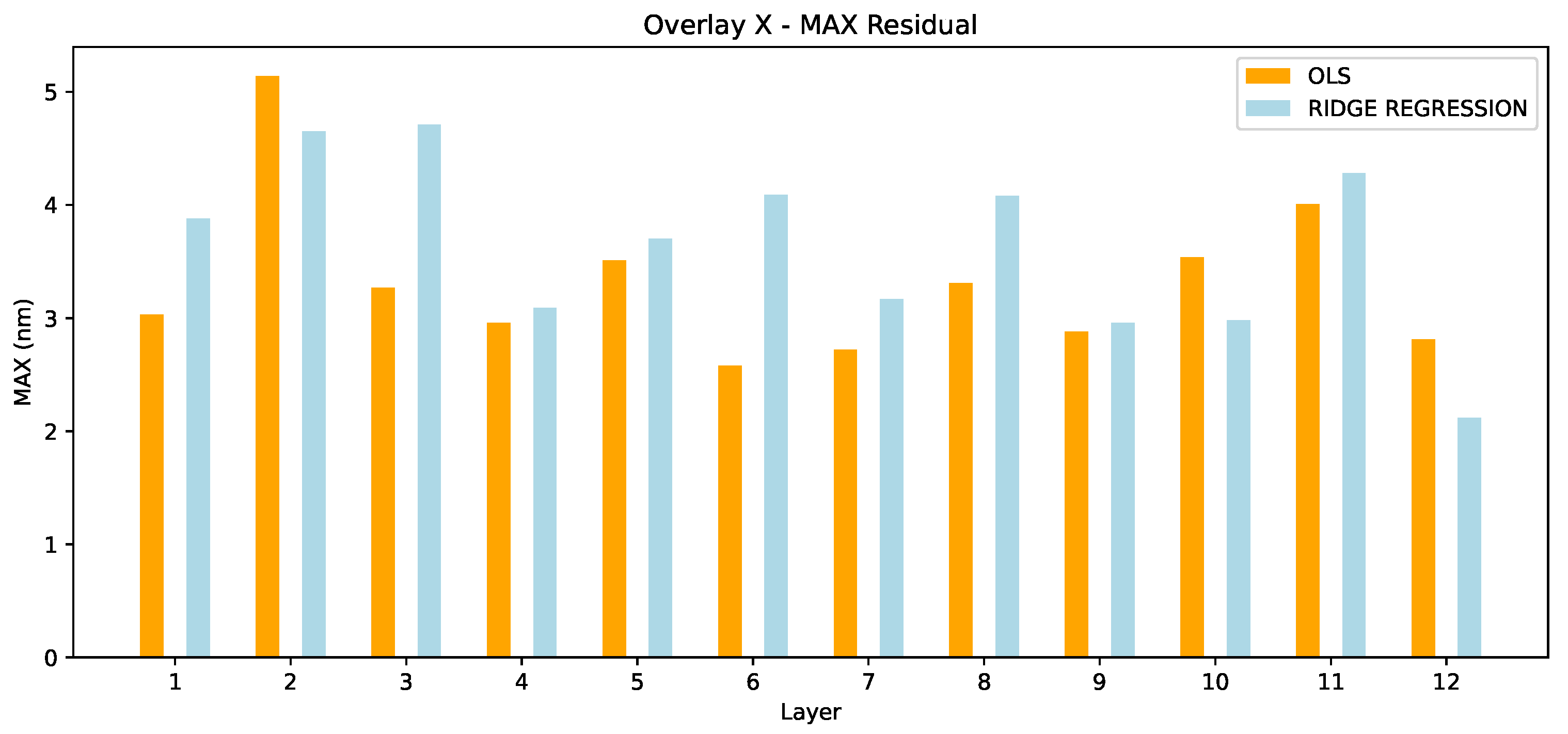
The max residuals in Overlay X are compared in
Figure 7. Here, we observe a different pattern than in 99.7. OLS outperforms the ridge regression in 9/12 layers. From these results we can not yet draw a safe conclusion. It dependes which metric we value most (99.7 vs. max) and this actually depends on the use case. However, the superiority of ridge regression in 99.7 only is an interesting conclusion already.
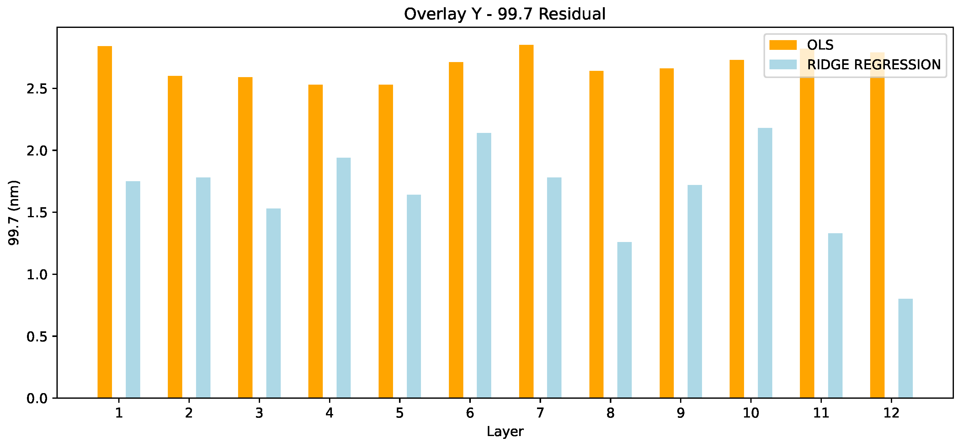
When checking the Overlay in Y we draw a more clear picture of the situation. As presented in
Figure 8 Ridge Regression ourtperforms significantly the OLS in all 12 layers. On average this is a 1.04 nm improvement. In this case the superiority of Ridge Regression is clear.
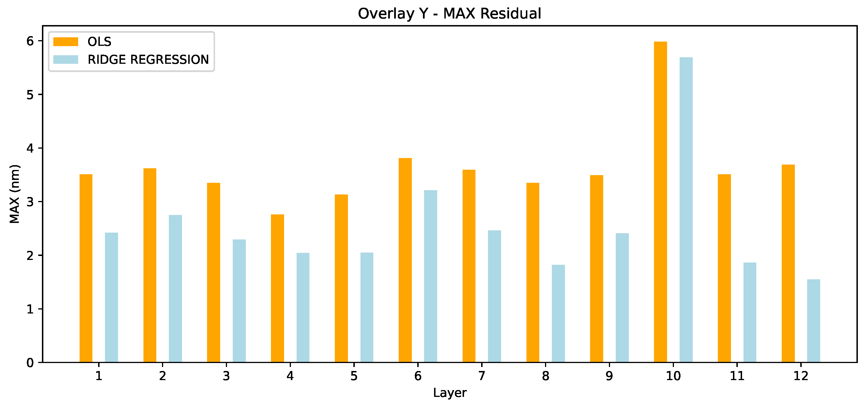
Similarly, in Overlay MAX we observe Ridge Regression outperforming OLS in all wafers with an average improvement of 1.10 nm.
The interesting conclusion, which verifies our hypothesis, is that Ridge Regression significantly outperforms OLS especially in Overlay Y. This makes sense since we already showed that the parameters which exhibit multicollinearity are almost double in Overlay Y than in Overlay X.
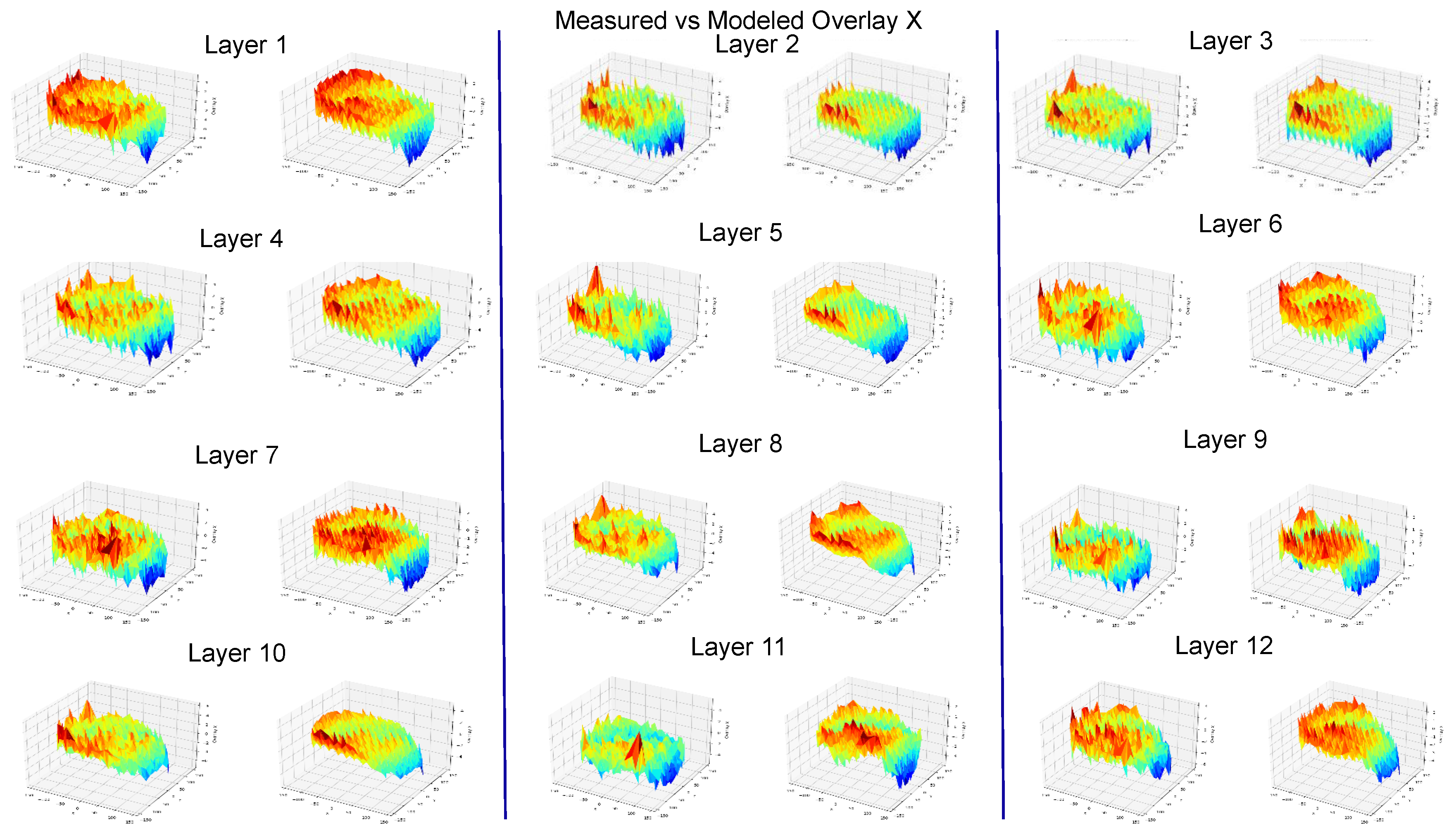
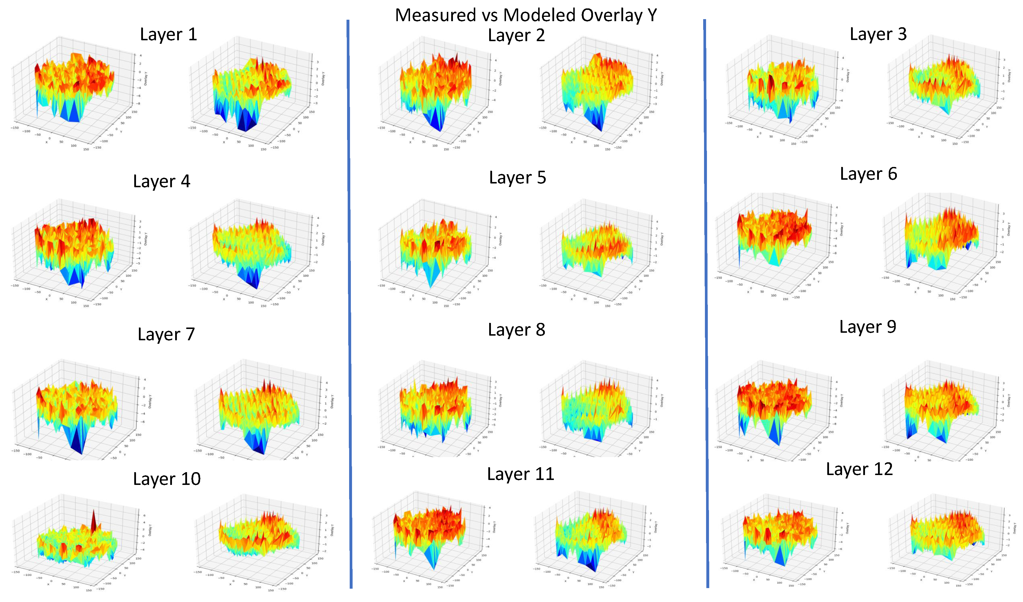
In
Figure 10 and
Figure 11 we present the measured vs. modeled Overlay X and Y for all the 12 layers.
4. Conclusion & Future Work
Ridge Regression results indicate an obvious superiority over OLS when the data exhibit multicollinearity. Especially in Overlay X where this phenomenon is more intense Ridge Regression outperforms OLS in every single layer. In the end, the overall improvement in 99.7 is 1.04 nm and in the max 1.10 nm. Such performance improvement in sub-nanometer level of precision can not be ignored. It is clear that OLS needs to be enhanced for similar datasets. One potential direction for future work would be the investigation of improving the model itself, either by reducing the features or by dynamically, during wafer production, select the most informative ones depending on the state of the process.
Author Contributions
Conceptualization, A.M.; methodology, A.M., C.G. and P.A.; software, A.M.; writing—original draft preparation, A.M.; writing—review and editing, A.M., P.A. and C.G.; supervision, A.B.; All authors have read and agreed to the published version of the manuscript.
Funding
This research received no external funding.
Data Availability Statement
The data presented in this study are not publicly available due to IP protection reasons.
Conflicts of Interest
The authors declare no conflict of interest.
References
- Moore’s Law Inspires Intel Innovation. Available online: https://www.intel.com/content/www/us/en/history/museum-gordonmoore-law.html.
- Jacobs, I. S. ”Fine particles, thin films and exchange anisotropy.” Magnetism (1963): 271-350.
- Lee, K. Y.; et al. Micromachining applications of a high resolution ultrathick photoresist. Journal of Vacuum Science & Technology B: Microelectronics and Nanometer Structures Processing, Measurement, and Phenomena 1995, 13, 3012–3016. [Google Scholar]
-
Fundamental Principles Of Optical Lithography: The Science Of Microfabrication; Wiley: Chichester, UK, 2012.
- Geng, H. Semiconductor Manufacturing Handbook, 2nd ed.; McGraw-Hill Educ: New York, NY, USA, 2018. [Google Scholar]
- Djurdjanovic, D.; Mears, L.; Niaki, F.A.; Haq, A.U.; Li, L. State of the art review on process, system, and operations control in modern manufacturing. ASME J. Manuf. Sci. Eng 2018, 140, 061010. [Google Scholar] [CrossRef]
- Hsueh, B.Y.; et al. “High order correction and sampling strategy for 45nm immersion lithography overlay control,” in Proc. SPIE Metrol. Inspection Process Control Microlithography XXII, vol. 6922, Mar. 2008, Art. no. 69222Q. [CrossRef]
- Choi, D.; et al. “Optimization of high order control including overlay, alignment, and sampling,” in Proc. SPIE, vol. 6922. San Jose, CA, USA, Feb. 2008, Art. no. 69220P. [CrossRef]
- H. Lin, B. H. Lin, B. Lin, J. Wu, S. Chiu, C.-C. Huang, J. Manka, et al., (2008). Improve overlay control and scanner utilization through high order corrections. Proceedings of SPIE - The International Society for Optical Engineering. 6922. [CrossRef]
- van den Brink, M.A.; de Mol, C.G.M.; George, R.A. “Matching performance for multiple wafer steppers using an advanced metrology procedure,” in Proc. Integr. Circuit Metrol. Inspection Process Control II, vol. 0921,” Online (Bergh.) p. 180, Jan. 1988. [CrossRef]
- Haq, A.U.; Djurdjanovic, D. “Robust control of overlay errors in photolithography processes,” IEEE Trans. Semicond. Manuf., vol. 32, no. 3, pp. 320–333, Aug. 2019. [CrossRef]
- Chien, C.-F.; Chen, Y.-J.; Hsu, C.-Y.; Wang, H.-K. “Overlay error compensation using advanced process control with dynamically adjusted proportional-integral R2R controller,” IEEE Trans. Autom. Sci. Eng., vol. 11, no. 2, pp. 473–484, Apr. 2014. [CrossRef]
- F. Tan, T. F. Tan, T. Pan, Z. Li, and S. Chen, “Survey on run-to-run control algorithms in high-mix semiconductor manufacturing processes,” IEEE Trans. Industr. Inform., vol. 11, no. 6, pp. 1435–1444, Dec. 2015. [CrossRef]
- J. Yu and S. Qin, “Variance component analysis based fault diagnosis of multi-layer overlay lithography processes,” IIE Trans., vol. 41, no. 9, pp. 764–775, 2009. [CrossRef]
- F. He and Z. Zhang, “An empirical study-based state space model for multilayer overlay errors in the step-scan lithography process,” RSC Adv., vol. 5, no. 126,103901–103906, 2015. [CrossRef]
- F. He and Z. Zhang, “State space model and numerical simulation of overlay error for multilayer overlay lithography processes,” in Proc. 2nd Int. Conf. Image Vis. Comput. (ICIVC), 2017, pp. 1123–1127. [CrossRef]
- M. Khakifirooz, M. M. Khakifirooz, M. Fathi, and C.-F. Chien, “Partially observable Markov decision process for monitoring multilayer wafer fabrication,” IEEE Trans. Autom. Sci. Eng., vol. 18, no. 4, pp. 1742–1753, Oct. 2021. [CrossRef]
- A. Magklaras, P. A. Magklaras, P. Alefragis, C. Gogos, C. Valouxis, and A. Birbas, “A Genetic Algorithm-Enhanced Sensor Marks Selection Algorithm for Wavefront Aberration Modeling in Extreme-UV (EUV) Photolithography,” Information (Basel), vol. 14, no. 8, p. 428, 2023. [CrossRef]
- Magklaras, A.; Gogos, C.; Alefragis, P.; Valouxis, C.; Birbas, A. Sampling Points Selection Algorithm For Advanced Photolithography Process. In Proceedings of the 2022 7th South-East Europe Design Automation, Computer Engineering, Computer Networks and Social Media Conference (SEEDA-CECNSM), Ioannina, Greece, 2022; pp. 1–5. [Google Scholar] [CrossRef]
- Zhang, H.; Feng, T.; Djurdjanovic, D. “Dynamic Down Selection of Measurement Markers for Optimized Robust Control of Overlay Errors in Photolithography Processes,” IEEE Trans. Semicond. Manuf., vol. 35, no. 2, pp. 241–255, 2022. [CrossRef]
- S.-C. Horng and S.-Y. Wu, “Compensating the overlay modeling errors in lithography process of wafer stepper,” in Proc. IEEE Conf. Ind. Electron. Appl. (ICIEA), Taichung, Taiwan, Jun. 2010, pp. 1399–1404.
- G.C. McDonald, “Ridge regression.”, Wiley Interdisciplinary Reviews: Computational Statistics 1.1 (2009): 93-100.
|
Disclaimer/Publisher’s Note: The statements, opinions and data contained in all publications are solely those of the individual author(s) and contributor(s) and not of MDPI and/or the editor(s). MDPI and/or the editor(s) disclaim responsibility for any injury to people or property resulting from any ideas, methods, instructions or products referred to in the content. |
© 2024 by the authors. Licensee MDPI, Basel, Switzerland. This article is an open access article distributed under the terms and conditions of the Creative Commons Attribution (CC BY) license (http://creativecommons.org/licenses/by/4.0/).
