Preprint
Article

Research on Bearing Fault Diagnosis Methods Based on Various Convolutional Neural Network Architectures

Altmetrics

Downloads

60

Views

33

Comments

0

This version is not peer-reviewed

Submitted:

12 September 2024

Posted:

13 September 2024

You are already at the latest version

Alerts
Abstract
Bearing fault diagnosis is crucial for ensuring the stable operation of mechanical equipment. With the continuous development of deep learning technology, Convolutional Neural Networks (CNNs) have demonstrated significant advantages in the field of fault diagnosis. This paper proposes a new method that combines various CNN architectures to improve the accuracy of bearing fault diagnosis. We designed five different convolutional network structures, including SerConv, ResConv, One-Shot Aggregation Convolution (OSAConv), Cross-Stage Aggregation Convolution (CSAConv), and MD-DAConv. Experimental results on the Case Western Reserve University (CWRU) bearing dataset show that the proposed method exhibits high accuracy and robustness in fault diagnosis. The results indicate that strategies such as multi-directional, multi-scale, and residual connections play a crucial role in enhancing the depth and breadth of feature extraction, while simple and effective feature fusion and information transmission mechanisms are key to ensuring the robustness and generalization ability of the model.
Keywords: 
Subject: Engineering  -   Electrical and Electronic Engineering

1. Introduction

With the continuous development of mechanical equipment, the internal structure of these systems has become increasingly sophisticated. Bearings, as critical components, are essential for the stable and efficient operation of the equipment. Bearing failures can severely impact equipment performance, leading to significant safety risks and economic losses. Therefore, monitoring and diagnosing bearing faults to detect issues promptly is of paramount importance [1,2,3].
In recent years, with the advancement of machine learning technologies, deep learning has increasingly been applied in the field of fault diagnosis. Compared to traditional fault detection methods, such as commonly used techniques including Support Vector Machines (SVM) [4,5,6], Random Forests [7,8,9], and BP Neural Networks [10,11,12], some deep learning methods significantly improve fault diagnosis accuracy while reducing human labor. Examples of such methods include Recurrent Neural Networks (RNN) [13,14,15], Convolutional Neural Networks (CNN) [16,17,18], and Deep Belief Networks (DBN) [19,20,21]. CNN, a biologically inspired variant of neural networks, offers powerful feature learning capabilities for classification problems. Current bearing fault diagnosis requires comprehensive analysis of various data types, such as vibration, sound, and temperature, to draw conclusions. Therefore, CNNs have become a research focus in the fault diagnosis field due to their strong feature extraction, autonomous learning, and prediction capabilities.
In previous studies, CNNs have been widely applied in the field of fault diagnosis [22]. However, CNNs were initially proposed to solve object detection and image classification problems. Currently, research on applying CNNs’ object detection capabilities to fault diagnosis is limited but has achieved some results. For instance, Wang et al. [23] designed a method to convert time-domain vibration signals into RGB 3D images using morphological operations, then input the converted images into the AlexNet CNN, achieving a certain level of accuracy. Shi et al. [24] proposed a fault diagnosis method combining CEEMDAN and CNN-SVM, utilizing 2D grayscale images for analysis to achieve fault diagnosis. Li et al. [25] discussed the use of an improved YOLOv8 model for diagnosing misfire faults in gasoline engines, with experimental results demonstrating higher recognition accuracy compared to other methods. Liu et al. [26] proposed an improved residual network for mechanical fault recognition through multi-channel weighting and used the GAF algorithm to convert vibration signals into feature images, achieving fault diagnosis for rolling bearings.
In recent years, significant progress has been made in the field of traditional CNN structure improvements. Howard et al. proposed MobileNets [27], a modification of the CNN architecture. Concurrently, Chollet [28] introduced the Xception algorithm, which replaces the inception module with depthwise separable convolutions. Xie et al. [29] designed a new network architecture model, ResNeXt, which improves computational precision while maintaining the same level of complexity. Zhang et al. [30] introduced ShuffleNet, a highly computationally efficient CNN that utilizes two new operations—pointwise group convolution and channel shuffle—greatly reducing computational costs while maintaining accuracy. It is evident that improvements to CNN architectures can significantly enhance computational efficiency.
As technology advances, more improved networks are being applied to diagnostic tasks. In recent years, deep learning technology has made remarkable progress in the field of fault diagnosis. Zhang J et al. proposed an intelligent fault diagnosis method combining time-frequency analysis and CNN, demonstrating its effectiveness under complex conditions [31]. Han et al. proposed a diagnostic framework combining Spatio-Temporal Feature Network (STPN) and CNN, effectively addressing fault diagnosis problems in complex systems, achieving good results in experiments [32]. Wang et al. proposed a method to improve fault recognition accuracy and robustness by fusing multi-sensor vibration signal images and using a bottleneck CNN for fault diagnosis [33]. He et al. proposed an Improved Multi-Scale CNN (IMSCNN) for bearing fault diagnosis by introducing convolution kernels with different dilation rates to expand the receptive field of the CNN. Experimental results showed that this method achieved higher diagnostic accuracy than traditional methods on the CWRU and PU datasets [34]. Gao et al. proposed a method combining multimodal data fusion and deep learning, using an Extended Wide First Layer Convolution Kernel (EWDCNN) and Long Short-Term Memory Network (LSTM) to improve diagnostic accuracy for rotating machinery in complex environments, demonstrating high diagnostic accuracy under different conditions [35]. Te et al. proposed a hybrid ST-CNN model by integrating the spatiotemporal pattern network (STPN) with convolutional neural networks (CNN), enhancing fault diagnosis performance in complex systems[36]. Zhang and Gu proposed a lightweight one-dimensional deep subdomain adaptation network (1D-LDSAN) for fast and accurate bearing fault diagnosis, with experimental results showing higher classification accuracy than mainstream transfer learning methods under different conditions [37]. Zhang et al. reviewed various fault diagnosis methods for mechanical rotating components, particularly the application of deep learning models, and mentioned that transfer learning-based methods can significantly improve diagnostic accuracy and efficiency [38]. Liang et al. proposed a new method based on deep learning that improves diagnostic accuracy by integrating information from different data sources [39]. Huang, T et al. proposed a novel fault diagnosis method combining a sliding window processing technique with a CNN-LSTM model, enhancing the performance of fault diagnosis by integrating feature extraction and time delay information of faults in complex systems. [40]. Hu et al. proposed an EfficientNet strategy based on attention mechanisms for bearing fault diagnosis in high-noise environments, achieving high diagnostic accuracy under different noise levels [41]. Zhang et al. proposed a bearing fault diagnosis method based on an improved dilated CNN (MAB-DrNet), enhancing feature extraction capabilities and classification accuracy in noisy environments by introducing the Maximum Average Block (MAB) module and the Global Residual Block (GRB) module [42]. Chen et al. proposed a bearing fault diagnosis method based on a stacked denoising autoencoder (SDAE), improving diagnostic accuracy in noisy environments through structural self-adaptation [43].
In the related work on bearing diagnosis, most network design strategies currently focus on increasing network depth to improve feature extraction capabilities across different layers. This paper proposes five efficient aggregation networks/extended neural networks by extending them horizontally and vertically and designing efficient dilated convolution layers to enhance the network’s feature extraction capabilities. The results indicate that multi-directional, multi-scale, and residual connection strategies play a crucial role in improving feature extraction depth and breadth. In contrast, simple and effective feature fusion and information transfer mechanisms are key to ensuring model robustness and generalization capabilities.

2. Feature Extraction Module

2.1. CNN Neural Network

Convolutional Neural Network (CNN) is a deep feedforward neural network model with strong automatic feature extraction capabilities. Its basic structure consists of an input layer, convolutional layers, pooling layers, fully connected layers, and an output layer.
(1) Input layer
The CNN model is a supervised learning model that requires learning under the supervision of sample labels. Therefore, the input consists of samples X and sample labels Y . For example, for a C-class classification problem, the model input, which is defined as Equation (1):
X , Y = { x i , y i } N
where N is the number of samples input into the model, x i is the iii-th sample, and yi is the class label corresponding to the i-th sample.
(2) Convolutional layer
The convolutional layer is the core component of the CNN model, implementing the concepts of local connectivity and weight sharing through convolutional kernels. The convolutional kernel slides horizontally and vertically along the coordinates of the input feature map, performing convolution operations with the data within the receptive field to extract structural features hidden within the data. The convolutional layer is organized in three dimensions: depth, width, and height. The width and height refer to the width and height of the convolutional kernel, which define the size of the local receptive field. Vibration signals are one-dimensional data, so the size of the convolutional kernel is k , with k constrained by the length of the input sample. Depth refers to the number of convolutional kernels. To extract different features from the input feature map, the convolutional layer performs convolution operations using a certain number of convolutional kernels, each with different weights, corresponding to different feature extractions. The convolution operation extracts features from the input feature map based on the size of the convolutional kernel and the stride. The process of feature extraction by the convolutional kernel is defined as follows:
f e a i , j L = q = 1 Q j = 1 J w k , j L f e a M , q L 1 + b j L , i = M + 2 p k s + 1
In the equation, w k , j L and b j L represent the weight and bias of the i -th convolutional kernel in the L -th convolutional layer, respectively. J is the number of convolutional kernels (the width of the convolutional layer), s is the stride, which is the distance the convolutional kernel slides over the input feature map, p is the padding size, f e a M , q L 1 is the q -th feature map of size M output by the L 1 -th layer, and f e a i , j L is the j -th convolutional kernel in the L -th convolutional layer, extracting a feature map of size i from the input feature map. Each convolutional kernel will find specific features at every position in the feature map, and the types of features learned are dynamically determined by the algorithm.
(3) Activation function
After the convolution operation, the results are processed by the activation function to obtain the corresponding output features. The activation function maps the originally linearly inseparable multidimensional features to another space, enabling the neural network to fit the nonlinear relationship between the input sample data and labels. The choice of activation function affects network training time and has a significant impact on performance on large datasets. Common activation functions in the field of fault diagnosis include the Sigmoid function, the Hyperbolic Tangent (Tanh) function, and the Rectified Linear Units (ReLU) function. The representations of these three types of functions, which are defined as follows:
f e a i , j L = s i g m o i d f e a i , j L 1 = 1 1 + e f e a i , j L 1 f e a i , j L = tanh f e a i , j L 1 = e f e a i , j L 1 e f e a i , j L 1 e f a i , j L 1 + e f e a i , j 1 f e a i , j L = T e L U f e a i , j L 1 = f e a i , j L 1 , z i , j L 21 > 0 0 , f e a i , j L 1 0
In the equations, f e a i , j L 1 and f e a i , j L represent the input and output of the function, respectively. The Sigmoid and Tanh functions are saturated nonlinear functions, mapping the input to the intervals [0,1] and [−1,1], respectively. During model training, if the neuron’s initialization or optimization enters the saturation region, the Sigmoid and Tanh functions are prone to the vanishing gradient problem, making further optimization difficult. Additionally, as the number of network layers increases, due to the chain rule, the derivatives of the multiplied Sigmoid and Tanh functions become increasingly small, hindering gradient backpropagation and reducing the network’s convergence speed, or even preventing the network from converging to an optimal state. In contrast, the ReLU function is a non-saturated nonlinear function that ensures all outputs are positive, effectively reducing the risk of vanishing gradients and gradient explosion during training. This alleviates the difficulty of training internal parameters in deep neural networks and facilitates faster network training. Therefore, the ReLU function is used as the activation function for all network layers.
(4) Pooling layer
The pooling layer, also known as the subsampling layer, is a network layer that performs pooling operations. After feature extraction by the convolutional layer, directly using these features for classification would face significant computational challenges and the risk of overfitting. Thus, it is necessary to perform pooling on the feature maps to reduce their data dimensionality. Pooling is a process of further abstracting information, similar to the feature extraction process of the convolutional layer. It involves sliding a window over the feature map and taking the statistical value of the local region corresponding to the window as the sampling value for that region. These values from the local regions are then concatenated to form a new feature map. Pooling operations are usually applied after convolutional layers, reducing feature dimensionality while preserving significant feature information and maintaining spatial invariance. Unlike convolution operations, pooling does not involve parameter settings and memory usage, greatly reducing the computational load. The pooling operation can be represented as:
f e a i , j L = f f e e i , j L 1 i = 0 , 1 , 2 , , i d s
where f is the pooling method, d is the size of the pooling function. When d < i , it indicates local pooling of the feature map, and when d = i , it indicates global pooling, where the entire feature map is pooled. s is the stride of the pooling function, and f e a i , j L is the output feature map after the corresponding pooling operation, with its size being i
(5) Fully connected layer
After multiple convolutional layers and max pooling layers, there are usually a few fully connected layers to integrate the local features extracted by the convolutional or pooling layers. The fully connected layer is a traditional multilayer perceptron that connects each neuron from the previous layer to every neuron in the next layer, generally using the ReLU function. For a one-dimensional input x i L 1 of length M , with N neurons in the fully connected layer, the output of each neuron can be represented as:
z j L = Re L U i = 1 M x i L 1 w j , i L + b j L , j = 1 , 2 , , N
In the equation, w j , i L is the connection weight from the i-th neuron in the L 1 -th layer to the j -th neuron in the L -th layer; x i L 1 is the input to the j -th neuron in the L -th layer; b j L is the bias of the j -th neuron in the L -th layer; and M and N represent the number of neurons in the L 1 -th layer and the L -th layer, respectively.
(6) Output layer
The output layer uses a classifier to output the model’s recognition results in the form of categories or probabilities. The most commonly used function is the nonlinear Softmax function, which is an extension of the logistic function and is typically used for multi-class classification problems. The Softmax function converts the extracted features into a probability distribution, using logarithmic probability values to estimate the likelihood of a sample belonging to a particular category. A higher value indicates greater confidence. It is represented as follows:
y ˜ i = s o f t max z i L 1 = p y i = 1 | z i L 1 ; θ p y i = 2 | z i L 1 ; θ p y i = c | z i L 1 ; θ = 1 j = 1 C exp z i L 1 exp z i L 1 exp z i L 1 exp z i L 1
where θ is the model’s parameters, and z i L 1 is the feature vector associated with the input x i . The Softmax function maps the feature set to a c-dimensional vector y ~ i , with each value in the vector ranging from (0,1) and the sum of all values in the vector equal to 1. Each element can be considered a category corresponding to the classifier parameters.

2.2. Construction of a Novel Network Architecture

To enhance feature extraction capabilities, this paper proposes five network structures based on the fundamental CNN architecture by stacking different convolutional layers and pooling layers, as well as multiple feature fusions and channel expansions. These structures effectively extract complex features from sample data as channels expand and increase. The main innovation of the network structures lies in the design of efficient expanded convolution layers, with each module employing multi-path convolution and feature concatenation strategies.

2.2.1. Serial Convolution (SerConv)

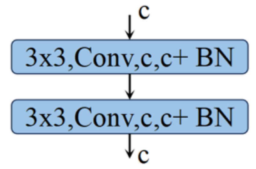
The SerConv network consists of two sequential convolutional blocks, each comprising a convolutional layer and a batch normalization layer. This setup stabilizes the learning process by normalizing the output of the convolutional layers, thereby enhancing the network’s generalization ability.
Let F x ; θ 1 represent the function applied by our convolutional block, where x denotes the block input, and θ is the parameters of the convolutional layer and batch normalization. This process can be defined mathematically as follows:
Convolutional Layer 1:
x 1 = F x ; θ 1 = B N C o n v x ; W 1 , b 1
where x 1 and b 1 are the weights and bias of the first convolutional layer, and B N is the batch normalization operation.
Convolutional Layer 2:
x 2 = F x 1 ; θ 2 = B N C o n v x 1 ; W 2 , b 2
where x 2 and b 2 are the weights and bias of the second convolutional layer.
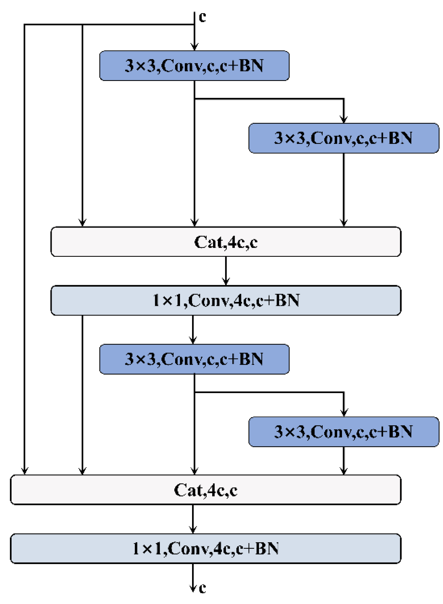
By sequentially connecting two convolutional blocks, the SerConv network can perform deeper feature extraction and processing on the input data without increasing computational complexity. Each convolutional block’s output undergoes batch normalization, which not only enhances the stability of the network during training but also improves the model’s ability to adapt to different data distributions to some extent. The specific structure is shown in Figure 1.

2.2.2. Residual Convolution (ResConv)

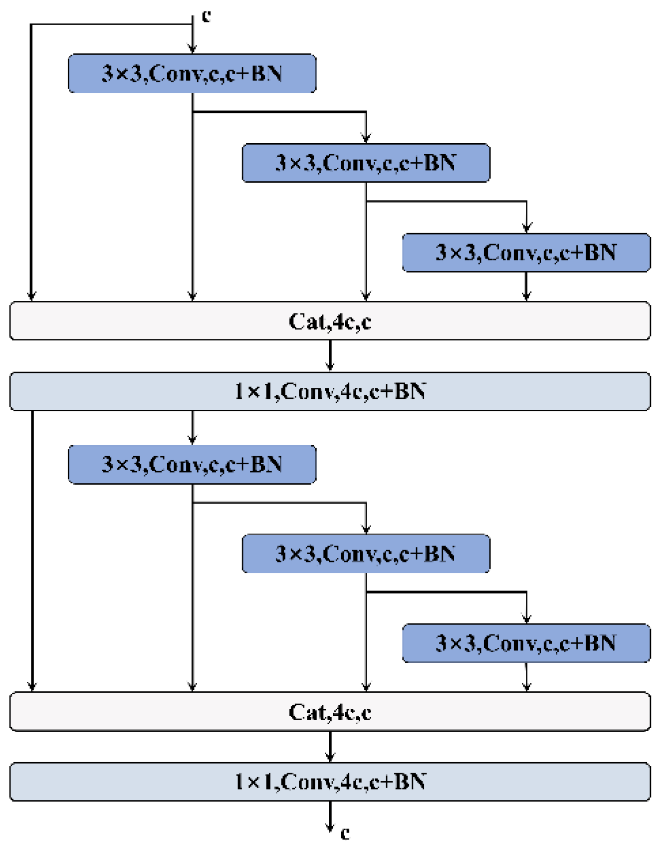
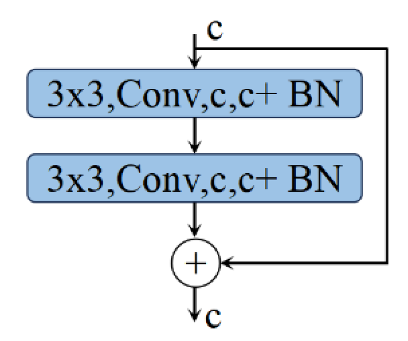
The ResConv structure consists of two consecutive convolutional blocks, each comprising a convolutional layer and a batch normalization layer. The residual connection is achieved by directly adding the input x to the output of the second convolutional block, merging the information before and after, thus allowing the network to learn incremental modifications to the input. The process for Convolutional Layer 1 and Convolutional Layer 2 is consistent with SerConv (Equations (1)–(2)), and x 3 is the final output.The process, which is defined as follows:
x 3 = x + x 2
By introducing residual connections into the convolutional network, the ResConv module increases the training depth of the network without compromising performance, effectively facilitating the learning of complex patterns. The specific structure is shown in Figure 2.

2.2.3. One-Shot Aggregation Convolution (OSAConv)

OSAConv is a novel deep learning network designed for feature data, with a core focus on processing one-dimensional sequence signals through deep feature extraction and efficient feature fusion. The network employs multiple stacked convolutional modules that feature multi-path convolution and feature concatenation mechanisms. Additionally, the number of channels is progressively increased after each layer, significantly enhancing the richness of features and the expressiveness of the model.
Each module utilizes multiple branches to extract features through consecutive convolution operations. These features are then concatenated with the original input, increasing the input information for subsequent layers. This design helps the model capture more refined local features and allows the network to acquire direct information from the original data before proceeding to deeper abstractions.
After each feature concatenation, the network performs feature fusion through convolutional layers, effectively reducing feature dimensions, alleviating computational burden, and ensuring the effectiveness and completeness of features in the depth direction. Below, this paper elaborates on the relevant formulas for the network structure:
In each module, the input first passes through a 3 × 3 convolutional layer to start the feature extraction process. For the nth layer of the module, its features (where n is the layer index) are obtained in the following manner:
y n , 1 = B N 1 C o n v 3 × 3 ( x )
Extract features on feature a through y n , 1 series of 3 × 3 convolutional layers, the process is defined as follows:
y n , 2 = BN 2 C o n v 3 × 3 y n , 1 y n , 3 = BN 3 C o n v 3 × 3 y n , 2
Subsequently, the first concatenation layer fuses the relevant features as follows,the process is defined as follows:
y c a t , 1 = C o n c a t y n , i ( i = 1 , 2 , 3 , 4 )
Here, Concat is the feature concatenation operation, which concatenates various feature maps along the channel dimension.
Subsequently, a 1 × 1 convolution is applied to the fused features for channel compression and feature integration to reduce the number of parameters and maintain computational efficiency,the process is defined as follows:
y o u t , 1 = BN 4 C o n v 1 × 1 y c a t , 1
The subsequent processing within the same module follows a similar pattern, further enhancing feature expression, the process is defined as follows::
y n , 4 = BN 5 Conv 3 × 3 y o u t , 1 y n , 5 = BN 6 Conv 3 × 3 y n , 4 y c a t , 2 = C o n c a t y o u t , 1 , y n , 4 , y n , 5 y o u t = BN 7 C o n v 1 × 1 y c a t , 2
In summary, the construction of OSAConv is completed as Figure 3.

2.2.4. Cross Stage Aggregation Convolution (CSAConv) Network

CSAConv is an innovative deep learning network designed for one-dimensional sequence signals. This architecture enhances the network’s feature extraction capability through cross-stage feature fusion combined with multi-scale convolutional kernels. The design aims to extract more diverse features through cross-stage feature fusion while maintaining computational efficiency. Specifically, the structure includes multiple 3 × 3 convolutional layers and 1 × 1 convolutional layers, which perform cross-stage convolution operations, ultimately concatenating the features to form a more powerful feature representation.
Below, this paper elaborates on the relevant formulas for the network structure:
The input feature x first passes through the first 3 × 3 convolutional layer and a batch normalization layer,the process is defined as follows:
y n , 1 = BN 1 C o n v 3 × 3 ( x )
Then it passes through another 3 × 3 convolutional layer for further feature extraction, the process is defined as follows:
y n , 2 = BN 2 C o n v 3 × 3 y n , 1
Subsequently, the relevant features are concatenated together,the process is defined as follows :
y c a t , 1 = C o n c a t y n , 1 , y n , 2
Subsequently, a 1 × 1 convolutional layer and a batch normalization layer are used for channel compression and feature integration, the process is defined as follows:
y o u t , 1 = BN 3 C o n v 1 × 1 y c a t , 1
At this point, the feature y o u t , 1 is passed through two more 3 × 3 convolutional layers to extract deeper-level features, the process is defined as follows:
y n , 3 = B N 4 C o n v 3 × 3 y o u t , 1 y n , 4 = B N 5 C o n v 3 × 3 y n , 1
Subsequently, the relevant features are further concatenated,the process is defined as follows:
y cat   , 2 = C o n c a t y out   , 1 , y n , 3 , y n , 4
Finally, the features are integrated through a 1 × 1 convolutional layer and a batch normalization layer to form the final output feature, the process is defined as follows:
y f i n a l = BN 6 C o n v 1 × 1 y c a t , 2
In summary, the construction of CSAConv is completed as Figure 4.

2.2.5. Multi-Directional Dense Aggregation Convolution (MD-DAConv) Network

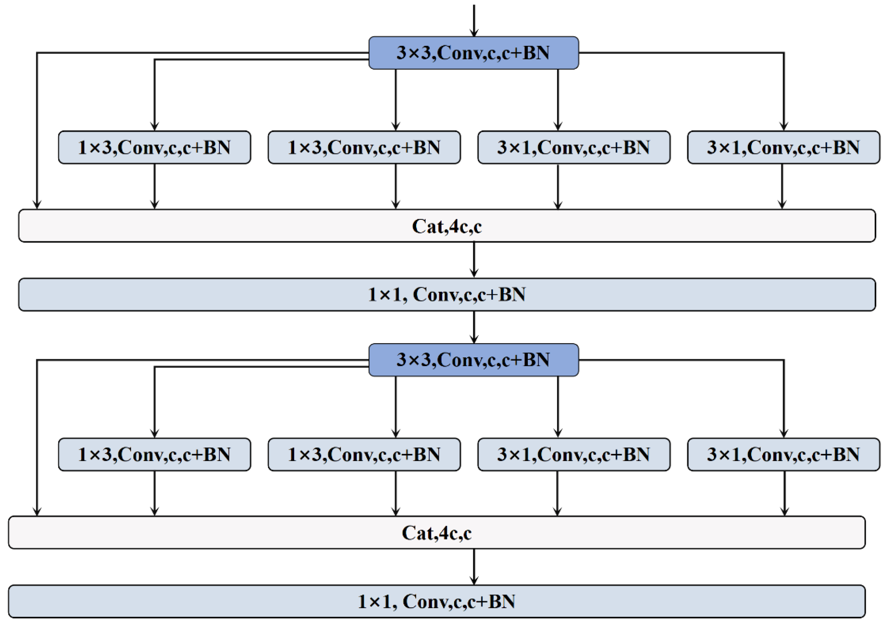
Currently, the use of dilated convolutional layers with different directions and scales has become a strategy for improving related networks. To verify whether this approach is suitable for fault diagnosis, this paper proposes a new convolutional structure called Multi-Directional Dense Aggregation Convolution (MD-DAConv). This structure aims to enhance the network’s feature extraction capabilities through multi-directional and multi-scale dilated convolutional layers combined with dense connections.
The design goal of this network is to extract more diverse features through multi-directional and multi-scale convolutional kernels while maintaining computational efficiency. Specifically, MD-DAConv includes multiple 3 × 3 convolutional layers, 1 × 1 convolutional layers, left and right dilated convolutional layers (1 × 3 and 3 × 1), and top and bottom dilated convolutional layers (3 × 1 and 1 × 3). The features from each layer are fused through dense connections to form a more powerful feature synthesis.
Below, this paper elaborates on the relevant formulas for the network structure:
In each module, the input x first passes through a 3 × 3 convolutional layer to begin the feature extraction process. For the nth layer of the module, its feature y n , 1  (where n is the layer index), which is defined as follows:
y n , 1 = BN 1 C o n v 3 × 3 ( x )
On feature y n , 1 , features are extracted through dilated convolutional layers in four directions:
y l e f t , 1 = BN 2 C o n v 1 × 3 y n , 1 y r i g h t , 1 = BN 3 C o n v 1 × 3 y n , 1 y u p , 1 = BN 4 C o n v 3 × 1 y n , 1 y d o w n , 1 = BN 5 C o n v 3 × 1 y n , 1
Subsequently, the concatenation operation, which is performed as follows:
y c a t , 1 = C o n c a t y n , 1 , y l e f t , 1 , y r i g h t , 1 , y u p , 1 , y d o w n , 1
Subsequently, channel compression and feature integration are performed through a 1 × 1 convolutional layer and a batch normalization layer, which is performed as follows:
y o u t , 1 = BN 6 C o n v 1 × 1 y c a t , 1
And feature y o u t , 1 is passed through a 3 × 3 convolutional layer and a batch normalization layer to extract deeper-level features, which is performed as follows:
y n , 2 = B N 7 C o n v 3 × 3 y o u t , 1
Subsequently, feature y n , 2 is passed sequentially through left-right and top-bottom dilated convolutional layers, which is performed as follows:
y l e f t , 2 = BN 8 C o n v 1 × 3 y n , 2 y r i g h t , 2 = BN 9 C o n v 1 × 3 y n , 2 y u p , 2 = BN 10 C o n v 3 × 1 y n , 2 y d o w n , 2 = BN 11 C o n v 3 × 1 y n , 2
Subsequently, all the features from the dilated convolutional layers are concatenated as follows:
y c a t , 2 = C o n c a t y n , 2 , y l e f t , 2 , y r i g h t , 2 , y u p , 2 , y d o w n , 2
Finally, integration is performed through a 1 × 1 convolutional layer and a batch normalization layer to form the final output feature, which is performed as follows:
y f i n a l = BN 12 C o n v 1 × 1 y c a t , 2
In the end, we can get network structure as shown in Figure 5:

2.3. Overall Network Model Structure

In the previous sections, we introduced various convolutional structures, including residual convolution (ResConv), multi-direction dense aggregation convolution (MD-DAConv), and so on. To compare the performance of different convolutional structures, we propose the following architecture as a general framework for subsequent experiments and validation as Figure 6.
The CNN model is composed of multiple convolutional layers and pooling layers, and it performs classification through fully connected layers and a Softmax layer at the end. The input layer of the model accepts one-dimensional signal data with a size of 1 × N, where NNN is the length of the input signal. The first convolutional layer uses 64 filters to perform convolution operations on the input signal, extracting initial features. Subsequently, the second convolutional layer further enhances the feature representation ability. The third convolutional layer increases the number of channels to 128 to capture more complex features, and the fourth convolutional layer continues the convolution operation on the features. The fifth convolutional layer increases the number of channels in the feature map to 256, and the sixth convolutional layer further enhances the feature representation ability. The seventh convolutional layer increases the number of channels in the feature map to 512 through convolution operations, and the eighth and ninth convolutional layers continue convolution operations on the features, further enhancing the feature representation ability.
The pooling layers use max pooling to reduce the size of the feature map by half, reducing computational load and the number of parameters while retaining the main features. Finally, the features extracted by the convolution and pooling operations are flattened into a one-dimensional vector through fully connected layers for feature fusion and classification, and the Softmax layer is used to output the final classification results.
2.4. Network Model Parameter Settings

The convolutional network structure data for the extended relevant layers is shown in the Table 1, Table 2, Table 3, Table 4 and Table 5:

3. Experimental Verification and Analysis

3.1. Hardware Parameters

To verify the bearing fault diagnosis capability of the proposed model, experimental evaluations were conducted on two bearing datasets. The experiments were implemented using the PyTorch deep learning framework. The computer configuration is as follows: Intel Core i7-8300H processor, NVIDIA GeForce 3060 graphics processor, and 16GB RAM.

3.2. CWRU Bearing Dataset

The Case Western Reserve University (CWRU) dataset is provided by the Bearing Data Center at Case Western Reserve University and is widely used as a standard reference for testing bearing diagnostic methods. The experimental setup for this dataset includes an induction motor, a torque sensor, test bearings, accelerometers, and a load motor. In this study, the focus is on the vibration signals of the drive-end bearing (bearing type SKF6205). Vibration acceleration signals of faulty bearings are measured by placing an accelerometer above each of the bearing housings at the fan end and drive end of the motor, followed by high-bandwidth amplification. This experiment uses SKF6205 deep groove ball bearings, including outer race faults, inner race faults, and rolling element faults with different fault diameters. The dataset used in this experiment corresponds to a load of 0, and specific dataset information is shown in Table 6.
The dataset includes four conditions: normal state, inner race fault, outer race fault, and rolling element fault. Each fault type has 3 fault sizes (0.007 inches, 0.014 inches, 0.021 inches), resulting in 9 fault conditions. Including the normal state, there are a total of 10 operating conditions. These 10 conditions are represented by category labels 0–9.
This study selects the vibration signals from the Drive End (DE) and the Fan End (FE) of the motor for subsequent training and testing, respectively, to compare the performance of the relevant structures.

3.3. Experimental Parameter Design

The network uses a batch size of 64 samples, 100 iterations, and a learning rate of 0.005. The accuracy function used is shown in Equation (30), and the categorical cross-entropy L is used as the loss function, as expressed in Equation (30).
L = c = 1 M y i c log p i c   Accuracy = T P + T N T P + T N + F P + F N
In the equations: M is the number of classes; y i c ​ is the indicator function for whether sample i belongs to class c (0 or 1), which is 1 if the true class of sample i equals class c , and 0 otherwise; p i c ​ is the predicted probability that sample i belongs to class c .

3.4. Experimental Results

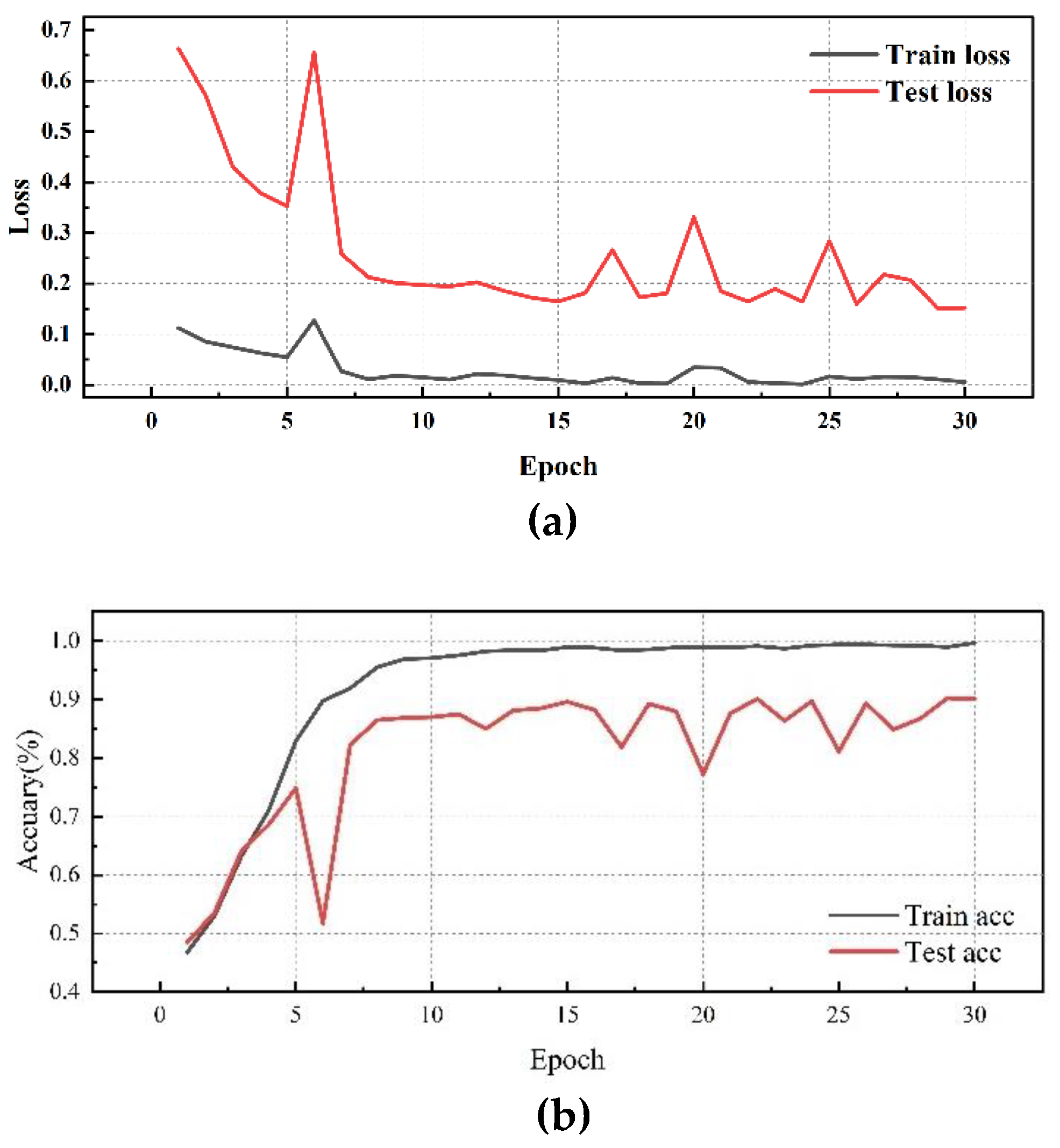
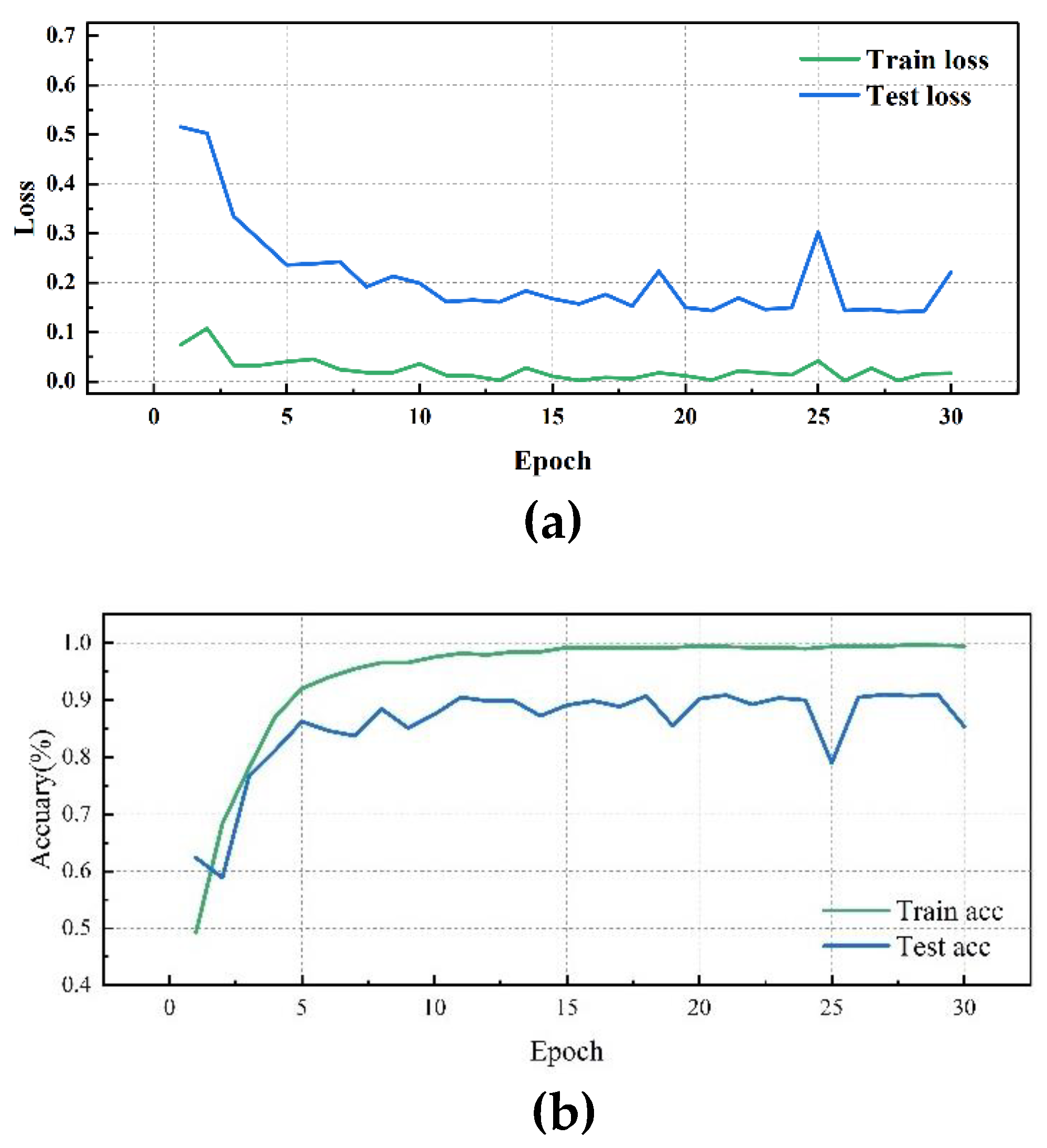
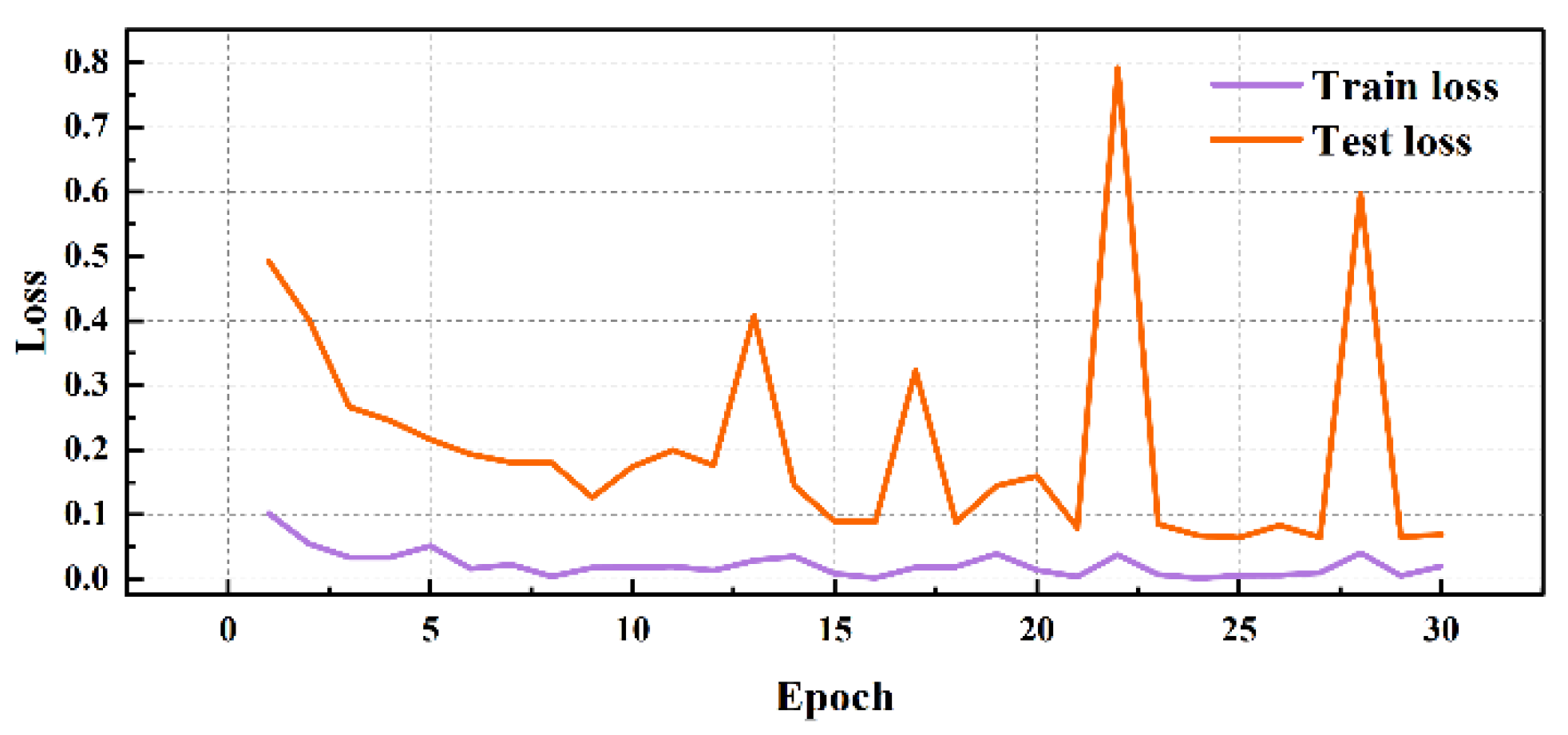
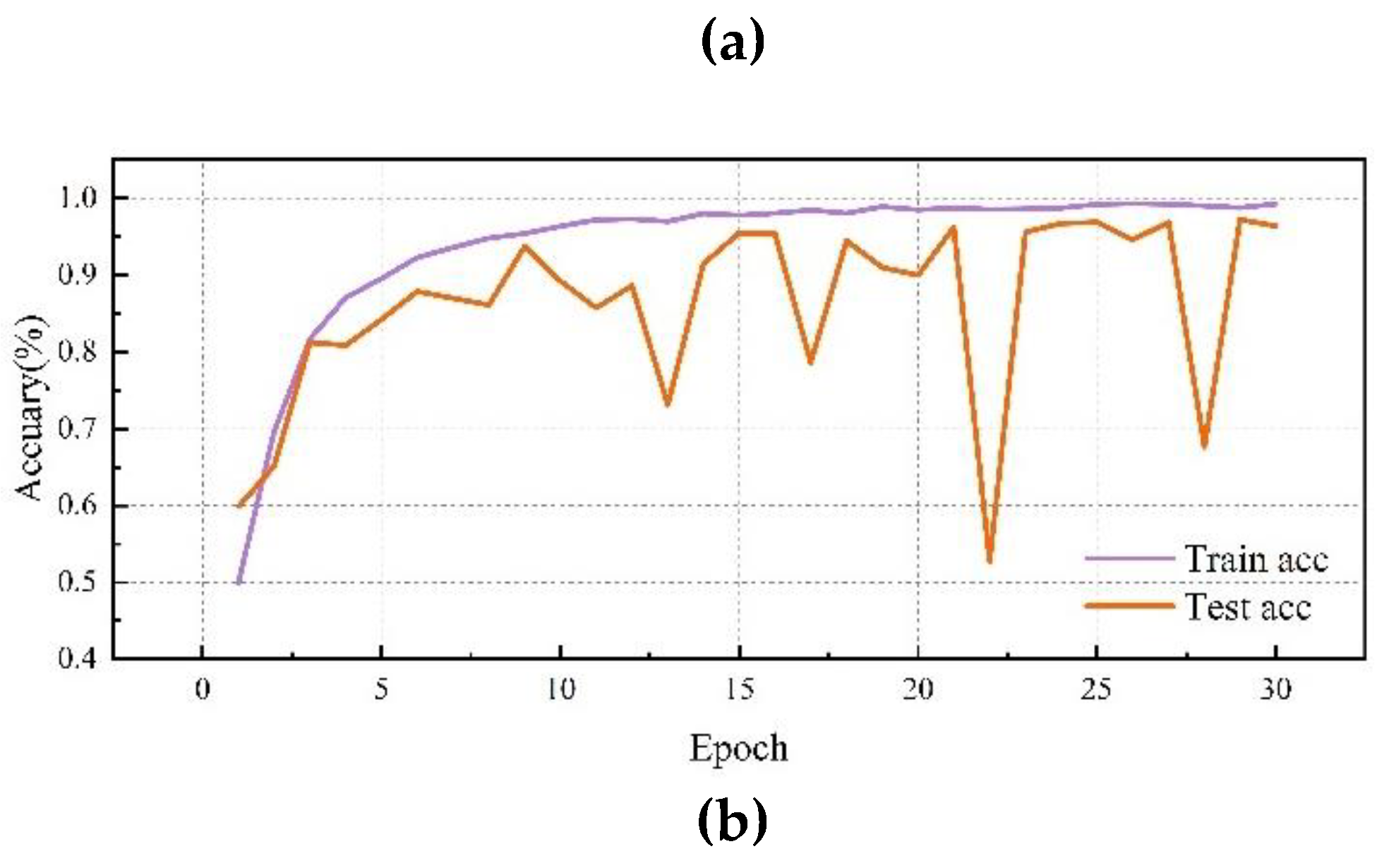
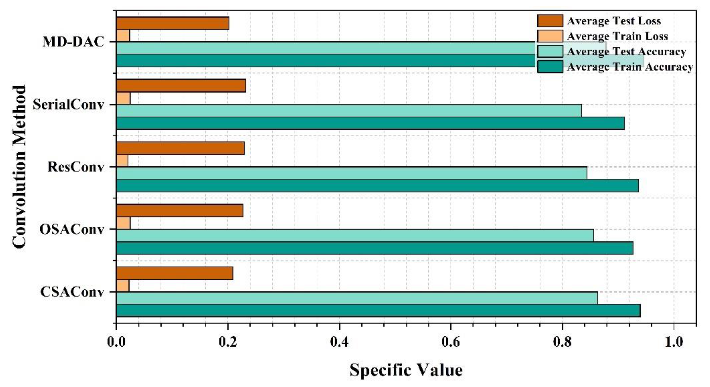
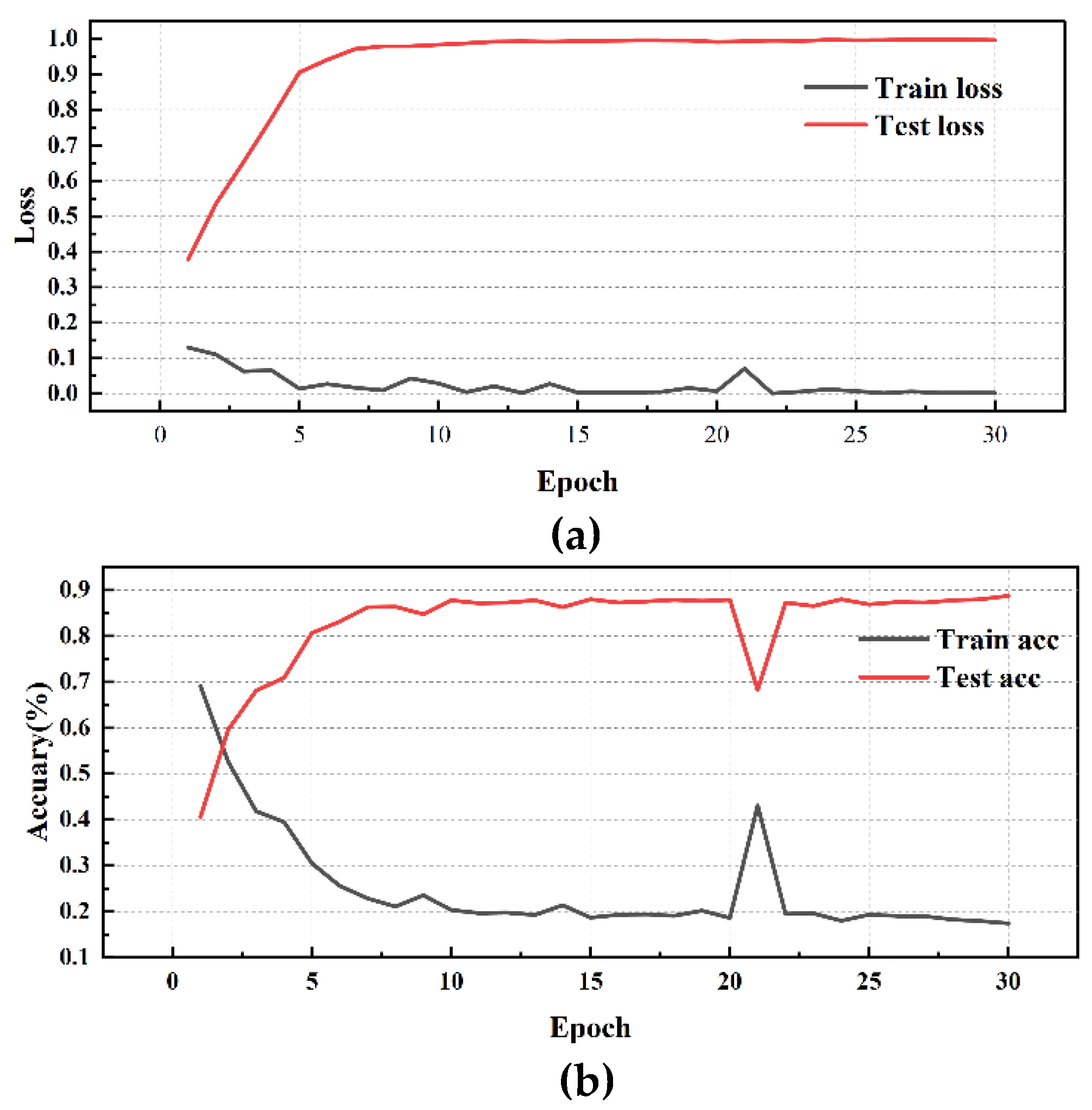
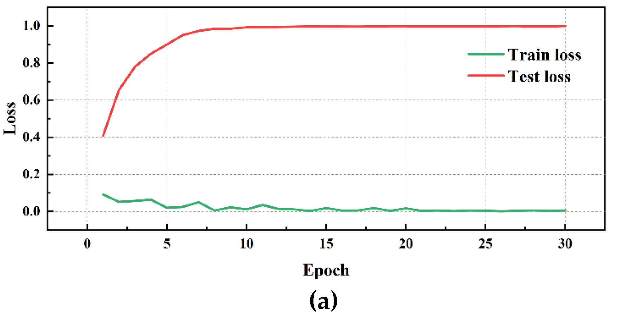
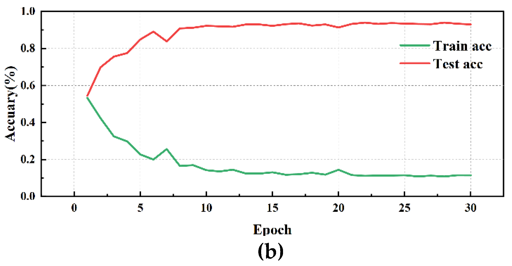
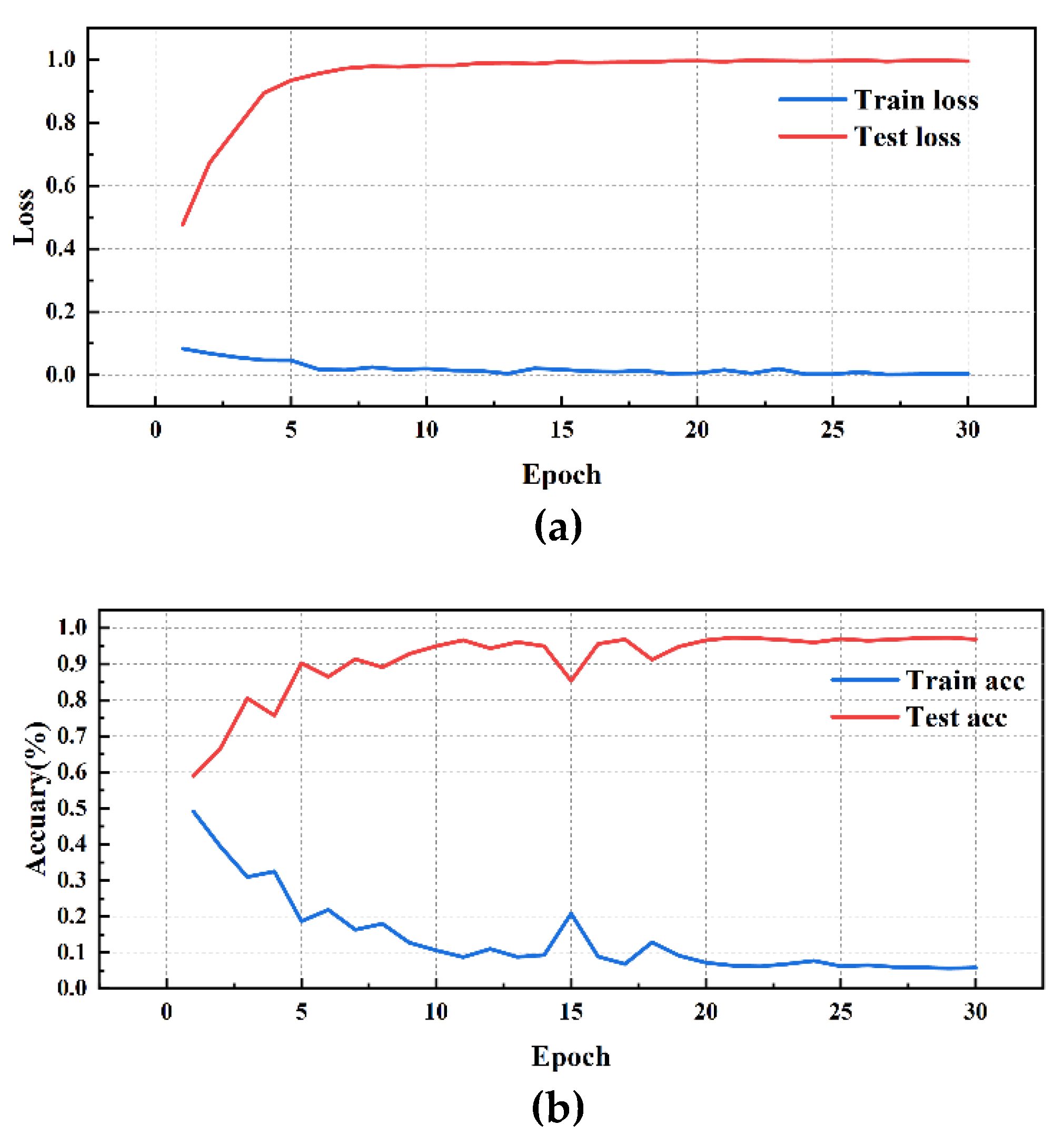
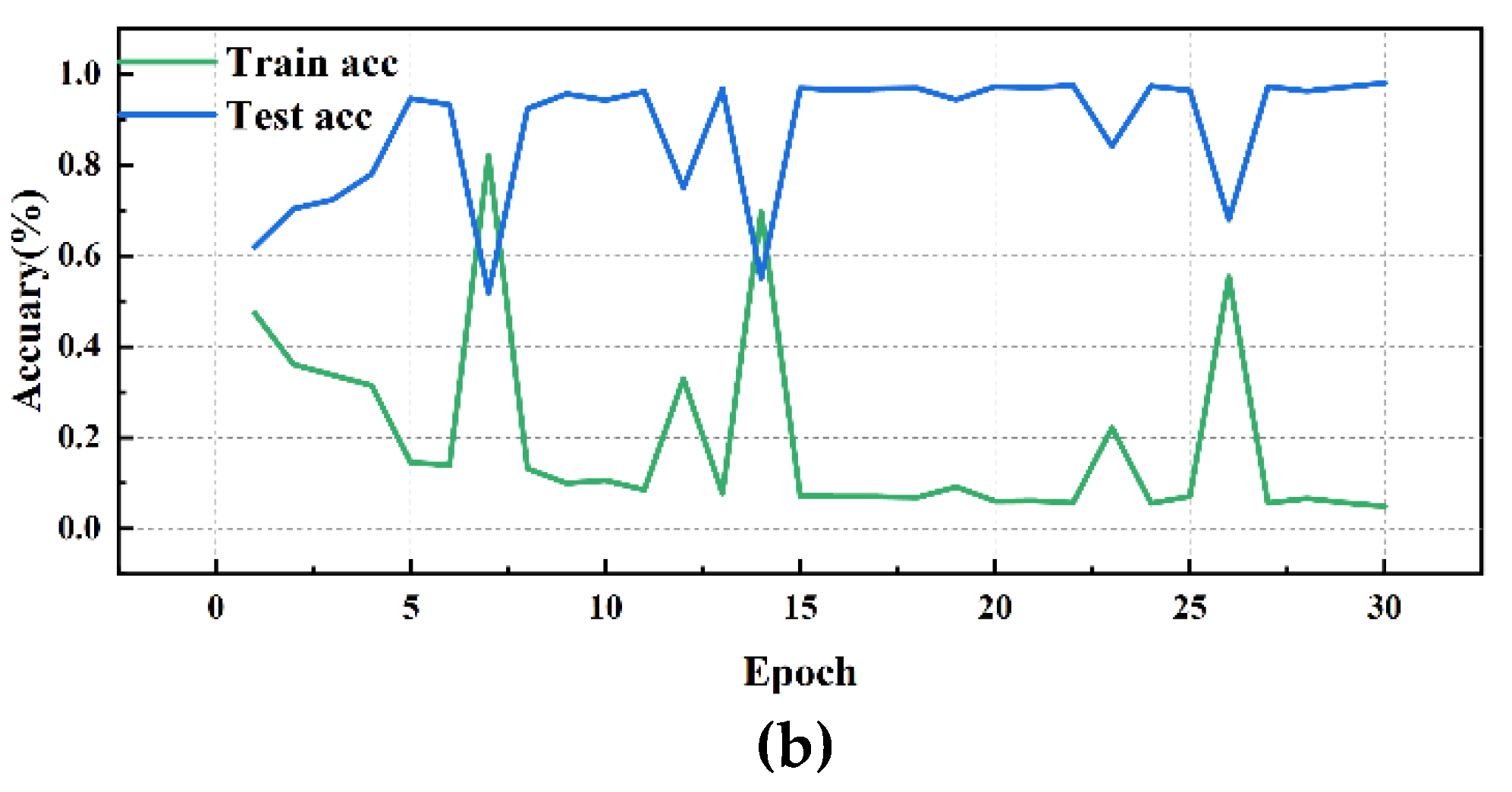
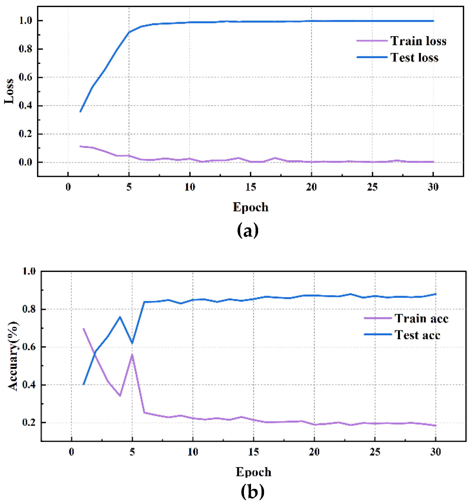
By comparing the performance of different convolution methods in diagnostic classification tasks, we have drawn some important conclusions. The table shows the average training accuracy, testing accuracy, training loss, and testing loss for each convolution method, as detailed Table 7 and Figure 7, Figure 8, Figure 9, Figure 10 and Figure 11:
By comparing the experimental results of different convolution methods, it can be observed that the network structure has a significant impact on bearing fault diagnosis performance. The MD-DAC network structure performs the best during the testing phase, with an average testing accuracy of 87.83%. Additionally, its relatively low testing loss (0.202199) indicates the model’s superior generalization ability. The OSA network structure has an average testing accuracy of 85.51%. Although slightly inferior to MD-DAC, its multi-path feature concatenation and channel expansion increase feature richness to some extent but also introduce feature redundancy issues, affecting its effectiveness in certain aspects. ResConv alleviates the vanishing gradient problem through residual connections, achieving an average testing accuracy of 84.42%. Despite being relatively high, it sometimes fails to capture all useful features, limiting performance improvement. The CSA network structure performs well during the testing phase, with an average testing accuracy of 86.35%. Its cross-hierarchical feature fusion can capture more global features, but the complexity of information transmission may introduce redundancy, affecting some of its performance. Despite achieving a stable training process through sequential convolution and batch normalization, Serial Convolution has an average testing accuracy of 83.44%, revealing issues of insufficient feature extraction depth and some information loss. Overall, the differences in the design of network structures concerning feature extraction, information transmission, and fusion strategies are the main reasons for performance variations. Strategies such as multi-direction, multi-scale, and residual connections play crucial roles in enhancing feature extraction depth and breadth, while simple and effective feature fusion and information transmission mechanisms are key to ensuring model robustness and generalization ability.
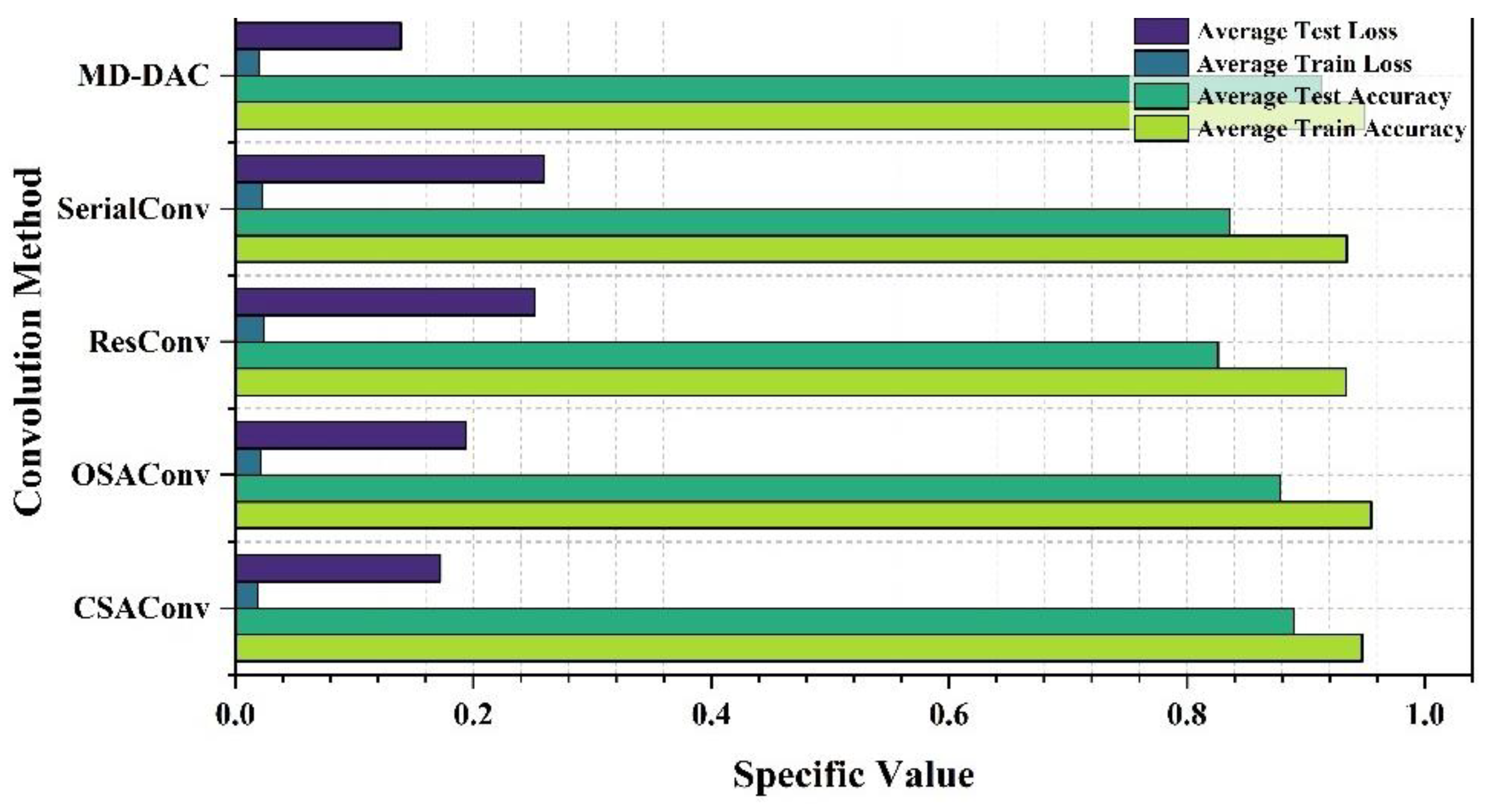
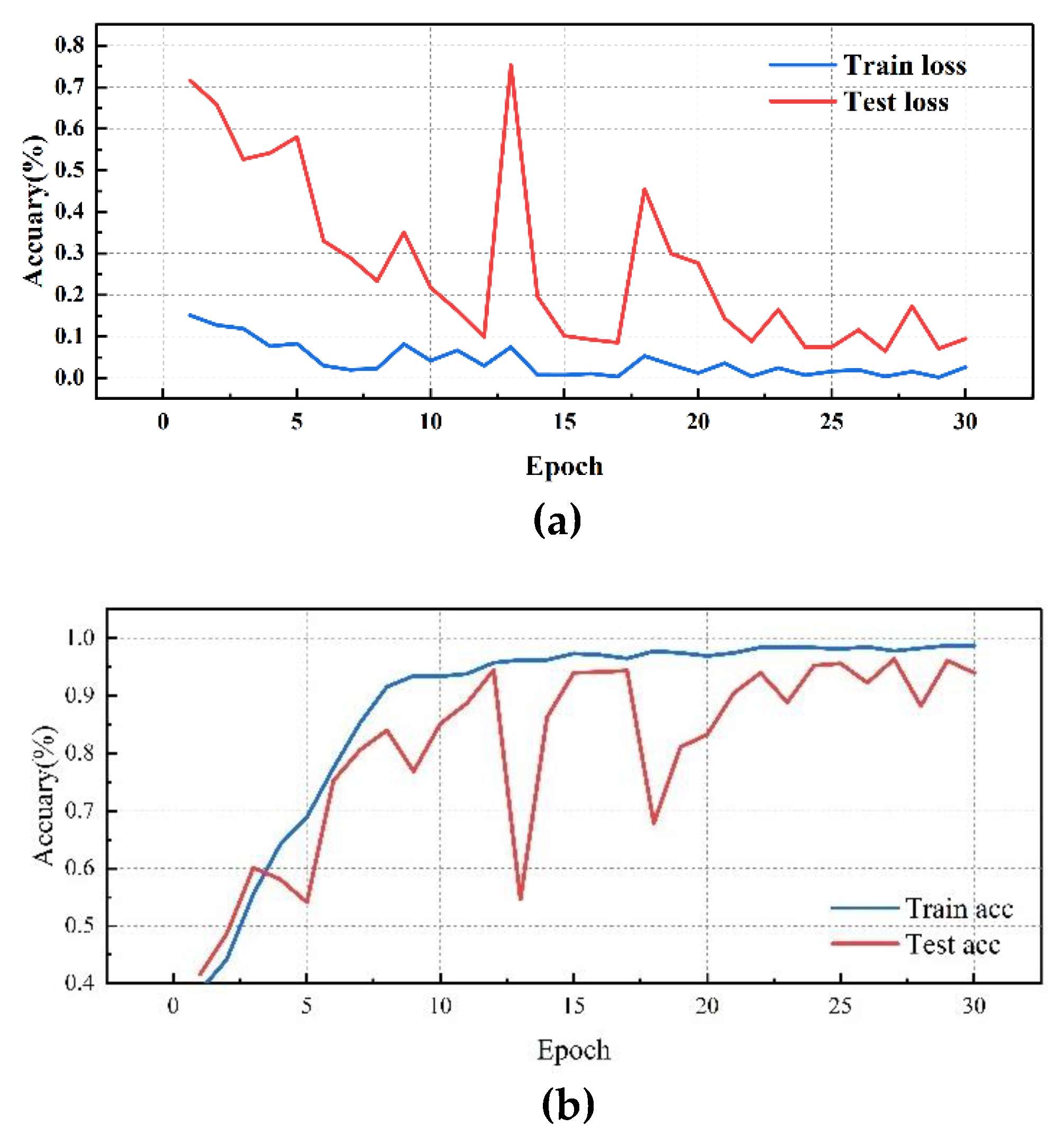
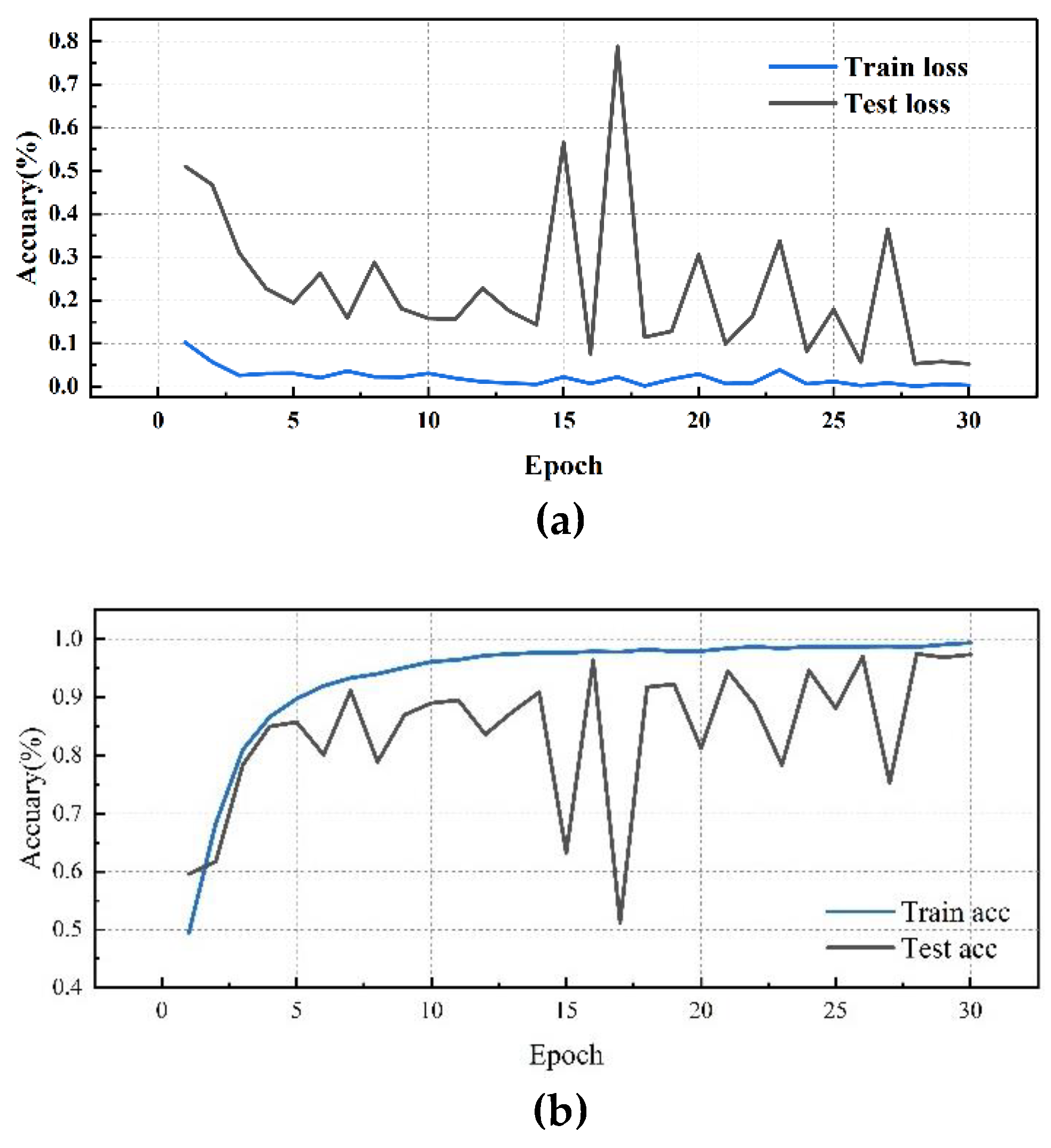
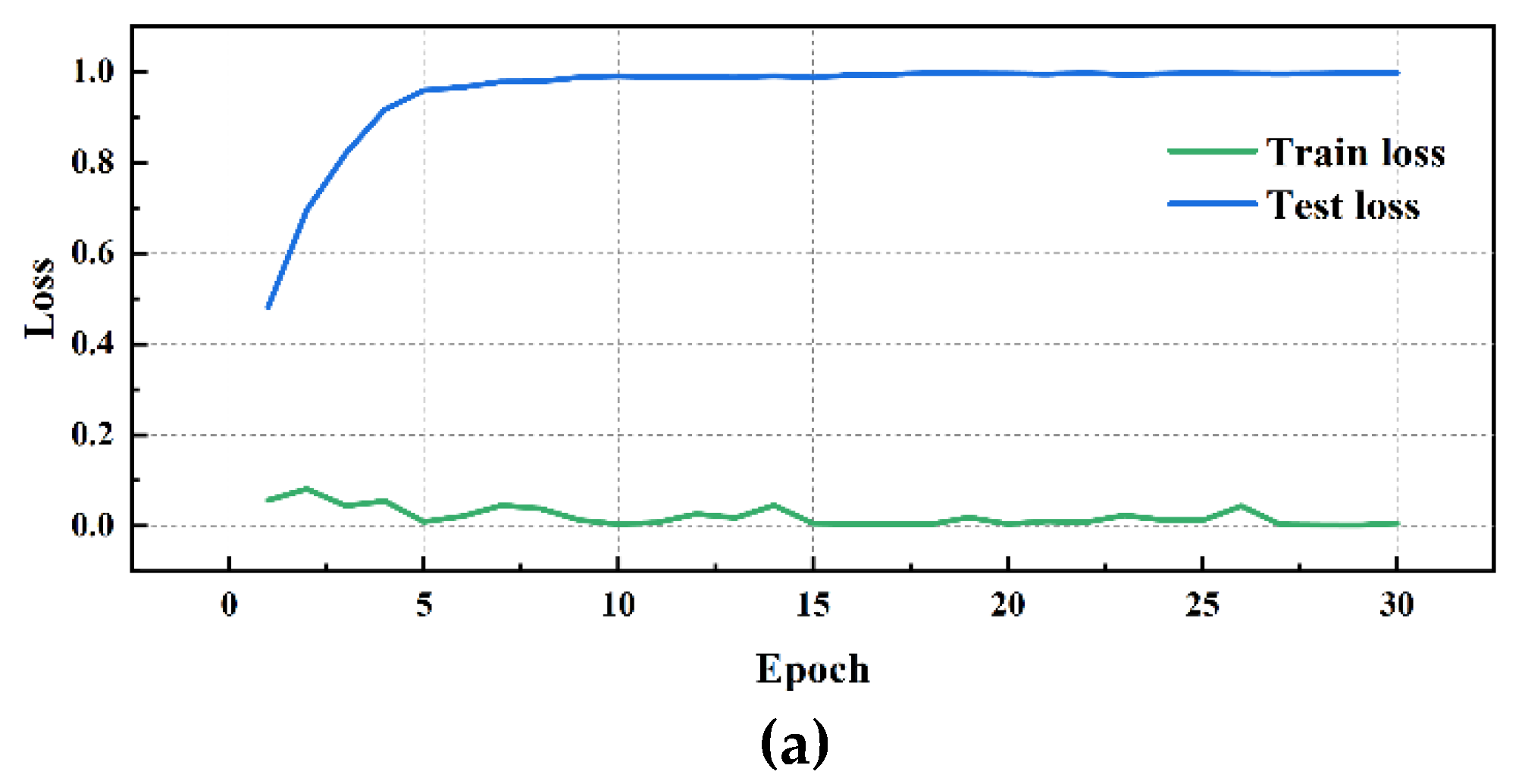
Subsequently, further testing experiments were conducted using DE data, the specific performance is shown in Table 8 and Figure 13, Figure 14, Figure 15, Figure 16, Figure 17 and Figure 18:
Simultaneously, by analyzing the experimental results of different convolution methods on DE data, it is found that the network structure has a significant impact on bearing fault diagnosis performance. Among them, the MD-DAC network structure performs the best during the testing phase, with an average testing accuracy of 91.29% and a low testing loss of 0.139110, demonstrating excellent generalization ability. In comparison, the OSAConv network structure has a testing accuracy of 87.85%, but with a testing loss of 0.193673, indicating that the feature redundancy issue still needs optimization. The CSAConv network structure performs well during the testing phase, with an average testing accuracy of 88.99%. Although its cross-hierarchical feature fusion design can capture more global features, the complexity may lead to some redundancy, affecting performance improvement. The SerialConv network structure achieves a stable training process through sequential convolution and batch normalization, but insufficient feature extraction depth results in an average testing accuracy of 83.61% and a testing loss of 0.259661, indicating problems of insufficient feature extraction depth and information loss. The ResConv network structure alleviates the vanishing gradient problem through residual connections, but its average testing accuracy is 82.62% with a testing loss of 0.251315, suggesting shortcomings in capturing useful features.
Based on the above experimental results, the advantage of MD-DAC lies in its combination of multi-directional and multi-scale convolution with dense connections. This design not only enhances the depth and breadth of feature extraction but also effectively reduces information loss. Although OSA’s multi-path feature concatenation improves feature richness, it also introduces redundancy. It may be beneficial to incorporate feature selection or feature compression mechanisms before feature concatenation to automatically filter out the most useful features and reduce redundancy. ResConv alleviates the vanishing gradient problem through residual connections but still has deficiencies in feature capturing. In the future, combining residual connections with attention mechanisms could enhance focus on key features and improve feature capturing ability. CSA captures more global features through cross-hierarchical feature fusion, but the complexity of information transmission may cause redundancy. Introducing inter-layer feature selection mechanisms and dynamically adjusting feature fusion strategies could improve the effectiveness of information transmission. Serial Convolution achieves a stable training process through sequential convolution and batch normalization, but the feature extraction depth is insufficient. Adding more layers in the sequential convolution or combining with multi-scale convolution could increase the depth of feature extraction.

4. Conclusion

Through the analysis of experimental results with different convolution methods, we found that network structure significantly impacts the performance of bearing fault diagnosis. The MD-DAC network structure, with its multi-directional and multi-scale feature extraction capabilities, performed the best during testing, demonstrating extremely high accuracy and generalization ability. Although OSA and CSA networks improved in terms of feature richness and global feature capture, issues with feature redundancy and the complexity of information transmission limited their further enhancement. ResConv alleviated the vanishing gradient problem through residual connections, but it still had deficiencies in capturing useful features. The feature fusion strategies of Doubleconv and Serial Convolution structures need optimization to better utilize diverse features and enhance model performance.
In summary, strategies such as multi-directional, multi-scale, and residual connections play a crucial role in the depth and breadth of feature extraction. At the same time, concise and effective feature fusion and information transmission mechanisms are key to ensuring model robustness and generalization ability. Future research can further optimize these network structures and explore more efficient feature fusion and information transmission methods to meet the application challenges in complex industrial environments.

Author Contributions

Conceptualization, Mingshen Xu, Bo Guan, Xinyu Shi and Jianghai Geng ; methodology, Mingshen Xu, Bo Guan, Jianghai Geng and Wanli Liu; software, Mingshen Xu, Xinyu Shi, and Runji Jiang; validation, Mingshen Xu, Wanli Liu, and Jingjia Tian; formal analysis, Mingshen Xu, Xinyu Shi, and Runji Jiang; investigation, Mingshen Xu, Bo Guan, and Xinyu Shi; resources, Runji Jiang, Wanli Liu, and Jingjia Tian; data curation, Bo Guan, Xinyu Shi, and Wanli Liu; writing—original draft preparation, Mingshen Xu, Bo Guan, Xinyu Shi, and Runji Jiang; writing—review and editing, Mingshen Xu, Wanli Liu, and Jingjia Tian; visualization, Mingshen Xu, Runji Jiang, and Jingjia Tian; supervision, Mingshen Xu, Bo Guan, Jianghai Geng and Runji Jiang; project administration, Mingshen Xu, Jianghai Geng and Jingjia Tian. All authors have read and agreed to the published version of the manuscript.

Funding

This research received no external funding

Institutional Review Board Statement

Not applicable.

Informed Consent Statement

Not applicable.

Data Availability Statement

The original data presented in this study are openly available in the Case Western Reserve University Bearing Data Center repository at https://csegroups.case.edu/bearingdatacenter/pages/welcome-case-western-reserve-university-bearing-data-center-website.

Conflicts of Interest

The authors declare no conflicts of interest.

References

  1. Tian, J.; Liu, L.; Zhang, F.; Ai, Y.; Wang, R.; Fei, C. Multi-domain entropy-random forest method for the fusion diagnosis of inter-shaft bearing faults with acoustic emission signals. Entropy 2020, 22, 57. [Google Scholar] [CrossRef] [PubMed]
  2. Jiang, D.; Wang, T.; Jiang, Y.; Liu, L.; Lin, J. Reliability analysis of motor spindle bearing based on operating condition. In Proceedings of the 2011 Third International Conference on Measuring Technology and Mechatronics Automation, Shanghai, China, 6–7 January 2011; pp. 989–992. [Google Scholar] [CrossRef]
  3. Jiang, D.; Wang, T.; Jiang, Y.; Liu, L.; Hu, M. Reliability assessment of machine tool spindle bearing based on vibration feature. In Proceedings of the 2010 International Conference on Digital Manufacturing & Automation, Changcha, China, 18–20 December 2010; pp. 154–157. [Google Scholar] [CrossRef]
  4. Kumar, K.K.; Srikanth, V.; Prasad, G.N.R.; Hazela, B.; Tamrakar, A.K. Fault detection on the 3-D printed objective surface by using the SVM algorithm. Mater. Today: Proc 2023. [Google Scholar] [CrossRef]
  5. Reddy, K.B.; Priya, M.V. ; Murugesan. In Power theft detection using novel linear SVM algorithm and compared with convolutional SVM algorithm for accuracy. In Proceedings of the 2022 14th International Conference on Mathematics, Actuarial Science, Computer Science and Statistics (MACS), Karachi, Pakistan, 12–13 November 2022; pp. 1–9. [Google Scholar] [CrossRef]
  6. Yang, Y.; Wang, J.; Yang, Y. Exploiting rotation invariance with SVM classifier for microcalcification detection. In Proceedings of the 2012 9th IEEE International Symposium on Biomedical Imaging (ISBI), Barcelona, Spain, 2–5 May 2012; pp. 590–593. [Google Scholar] [CrossRef]
  7. Xu, G.; Liu, M.; Jiang, Z.; Söffker, D.; Shen, W. Bearing fault diagnosis method based on deep convolutional neural network and random forest ensemble learning. Sensors 2019, 19, 1088. [Google Scholar] [CrossRef] [PubMed]
  8. Dong, L.; Du, H.; Mao, F.; Han, N.; Li, X.; Zhou, G.; Zhu, D.; Zheng, J.; Zhang, M.; Xing, L.; Liu, T. Very high resolution remote sensing imagery classification using a fusion of random forest and deep learning technique—subtropical area for example. IEEE J. Sel. Top. Appl. Earth Obs. Remote Sens. 2020, 13, 113–128. [Google Scholar] [CrossRef]
  9. Singh, T.; Mansour, R.R. Chalcogenide phase change material GeTe based inline RF SPST series and shunt switches. In Proceedings of the 2018 IEEE MTT-S International Microwave Workshop Series on Advanced Materials and Processes for RF and THz Applications (IMWS-AMP), Ann Arbor, MI, USA, 16–18 July 2018; pp. 1–3. [Google Scholar] [CrossRef]
  10. Tian, Y.; Cai, B.; Liu, Y. Research on BPNN-based SVM-DTC for direct drive PMSG wind turbine. In Proceedings of the 2021 China Automation Congress (CAC), Beijing, China, 22–24 October 2021; pp. 3098–3103. [Google Scholar] [CrossRef]
  11. Chen, B.; Xing, L.; Zhao, L.; Xie, Y.; Cai, Y.; Chen, X. Prediction model of commercial economic index based on BPNN optimization algorithm. In Proceedings of the 2020 International Conference on Computer Engineering and Application (ICCEA), Guangzhou, China, 18–20 March 2020; pp. 529–532. [Google Scholar] [CrossRef]
  12. Tsai, T.Y.; Chen, H.W. Apply BPNN with Kalman Filtering to the dynamic system identification. In Proceedings of the 2008 International Conference on Machine Learning and Cybernetics, Kunming, China, 12–15 July 2008; pp. 3188–3193. [Google Scholar] [CrossRef]
  13. Panchapagesan, S.; Park, D.S.; Chiu, C.C.; Shangguan, Y.; Liang, Q.; Gruenstein, A. Efficient knowledge distillation for RNN-transducer models. In Proceedings of the ICASSP 2021 - 2021 IEEE International Conference on Acoustics, Speech and Signal Processing (ICASSP), Toronto, ON, Canada, 6–11 June 2021; pp. 5639–5643. [Google Scholar] [CrossRef]
  14. Guo, Z.; Yang, M. TFFC-RNN: A new RNN based approach for bearing and misalignment compound fault. In Proceedings of the 2022 International Power Electronics Conference (IPEC-Himeji 2022- ECCE Asia), Himeji, Japan, 15–19 May 2022; pp. 2504–2509. [Google Scholar] [CrossRef]
  15. Zhang, X.; Luo, T. A RNN decoder for channel decoding under correlated noise. In Proceedings of the 2019 IEEE/CIC International Conference on Communications Workshops in China (ICCC Workshops), Changchun, China, 11–13 August 2019; pp. 30–35. [Google Scholar] [CrossRef]
  16. Yanagisawa, H.; Yamashita, T.; Watanabe, H. A study on object detection method from manga images using CNN. In Proceedings of the 2018 International Workshop on Advanced Image Technology (IWAIT), Chiang Mai, Thailand, 7–9 January 2018; pp. 1–4. [Google Scholar] [CrossRef]
  17. He, X.; Chen, Y. Optimized input for CNN-based hyperspectral image classification using spatial transformer network. IEEE Geosci. Remote Sens. Lett. 2019, 16, 1884–1888. [Google Scholar] [CrossRef]
  18. Daanouni, O.; Cherradi, B.; Tmiri, A. NSL-MHA-CNN: A novel CNN architecture for robust diabetic retinopathy prediction against adversarial attacks. IEEE Access 2022, 10, 103987–103999. [Google Scholar] [CrossRef]
  19. Wang, L.; Liu, H.; Pan, Z.; Xu, Y.; Fan, D.; Zhou, C.; Li, Y. Temperature demodulation for optical fiber F-P sensor based on DBNs with ensemble learning. Opt. Laser Technol. 2023, 162, 109275. [Google Scholar] [CrossRef]
  20. Jiang, D.; Wu, P.; Wang, F.; Sahli, H.; Verhelst, W. Audio visual speech recognition based on multi-stream DBN models with articulatory features. In Proceedings of the 2010 7th International Symposium on Chinese Spoken Language Processing, Tainan, Taiwan, 29 November–3 December 2010; pp. 190–193. [Google Scholar] [CrossRef]
  21. Chen, D.; Jiang, D.; Ravyse, J.; Sahli, H. Audio-visual emotion recognition based on a DBN model with constrained asynchrony. In Proceedings of the 2009 Fifth International Conference on Image and Graphics, Xi’an, China, 20–23 September 2009; pp. 912–916. [Google Scholar] [CrossRef]
  22. Lal Senanayaka, J.S.; Van Khang, H.; Robbersmvr, K.G. CNN based gearbox fault diagnosis and interpretation of learning features. In Proceedings of the 2021 IEEE 30th International Symposium on Industrial Electronics (ISIE), Kyoto, Japan, 20–23 June 2021; pp. 1–6. [Google Scholar] [CrossRef]
  23. Wang, Z.; Zhao, W.; Du, W.; Li, N.; Wang, J. Data-driven fault diagnosis method based on the conversion of erosion operation signals into images and convolutional neural network. Process Saf. Environ. Prot. 2021, 149, 591–601. [Google Scholar] [CrossRef]
  24. Shi, L.; Liu, W.; You, D.; Yang, S. Rolling bearing fault diagnosis based on CEEMDAN and CNN-SVM. Appl. Sci. 2024, 14, 5847. [Google Scholar] [CrossRef]
  25. Li, Z.; Qin, Z.; Luo, W.; Ling, X. Gasoline engine misfire fault diagnosis method based on improved YOLOv8. Electronics 2024, 13, 2688. [Google Scholar] [CrossRef]
  26. Liu, Z.; Yu, H.; Xu, K.; Miao, X. RMCW: An improved residual network with multi-channel weighting for machinery fault diagnosis. IEEE Access 2023, 11, 124472–124483. [Google Scholar] [CrossRef]
  27. Howard, A.G.; Zhu, M.; Chen, B.; Kalenichenko, D.; Wang, W.; Weyand, T.; Andreetto, M.; Adam, H. MobileNets: Efficient convolutional neural networks for mobile vision applications. arXiv preprint 2017, arXiv:1704.04861. [Google Scholar] [CrossRef]
  28. Chollet, F. Xception: Deep learning with depthwise separable convolutions. In Proceedings of the 2017 IEEE Conference on Computer Vision and Pattern Recognition (CVPR), Honolulu, HI, USA, 21–26 July 2017; pp. 1800–1807. [Google Scholar] [CrossRef]
  29. Xie, S.; Girshick, R.; Dollár, P.; Tu, Z.; He, K. Aggregated residual transformations for deep neural networks. In Proceedings of the 2017 IEEE Conference on Computer Vision and Pattern Recognition (CVPR), Honolulu, HI, USA, 21–26 July 2017; pp. 5987–5995. [Google Scholar] [CrossRef]
  30. Zhang, X.; Zhou, X.; Lin, M.; Sun, J. ShuffleNet: An extremely efficient convolutional neural network for mobile devices. In Proceedings of the 2018 IEEE Conference on Computer Vision and Pattern Recognition, Salt Lake City, UT, USA, 18–23 June 2018; pp. 6848–6856. [Google Scholar] [CrossRef]
  31. Zhang J, Zhang Q, Qin X, Sun Y. An intelligent fault diagnosis method based on domain adaptation for rolling bearings under variable load conditions. Proceedings of the Institution of Mechanical Engineers, Part C: Journal of Mechanical Engineering Science 2021, 235, 8025–8038. [Google Scholar] [CrossRef]
  32. Han, T.; Liu, C.; Wu, L.; Sarkar, S.; Jiang, D. An adaptive spatiotemporal feature learning approach for fault diagnosis in complex systems. Mech. Syst. Signal Process. 2019, 117, 170–187. [Google Scholar] [CrossRef]
  33. Wang, H.; Li, S.; Song, L.; Cui, L. A novel convolutional neural network based fault recognition method via image fusion of multi-vibration-signals. Comput. Ind. 2019, 105, 182–190. [Google Scholar] [CrossRef]
  34. He, J.; Wu, P.; Tong, Y.; Zhang, X.; Lei, M.; Gao, J. Bearing fault diagnosis via improved one-dimensional multi-scale dilated CNN. Sensors 2021, 21, 7319. [Google Scholar] [CrossRef]
  35. Gao, Y.; Kim, C.H.; Kim, J.M. A novel hybrid deep learning method for fault diagnosis of rotating machinery based on extended WDCNN and long short-term memory. Sensors 2021, 21, 6614. [Google Scholar] [CrossRef]
  36. Te, H.; Liu, C.; Wu, L.; Sarkar, S.; Jiang, D. An Adaptive Spatiotemporal Feature Learning Approach for Fault Diagnosis in Complex Systems. Mech. Syst. Signal Process. 2019, 117, 170–187. [Google Scholar] [CrossRef]
  37. Zhang, R.; Gu, Y. A Transfer Learning Framework with a One-Dimensional Deep Subdomain Adaptation Network for Bearing Fault Diagnosis under Different Working Conditions. Sensors 2022, 22, 1624. [Google Scholar] [CrossRef]
  38. Zhang, T.; Chen, J.; Li, F.; Zhang, K.; Lv, H.; He, S.; Xu, E. Intelligent fault diagnosis of machines with small & imbalanced data: A state-of-the-art review and possible extensions. ISA Trans. 2022, 119, 152–171. [Google Scholar] [CrossRef]
  39. Liang, P.; Wang, W.; Yuan, X.; Liu, S.; Zhang, L.; Cheng, Y. Intelligent fault diagnosis of rolling bearing based on wavelet transform and improved ResNet under noisy labels and environment. Eng. Appl. Artif. Intell. 2022, 115, 105269. [Google Scholar] [CrossRef]
  40. Huang, T. , Zhang, Q., Tang, X. et al. A novel fault diagnosis method based on CNN and LSTM and its application in fault diagnosis for complex systems. Artif Intell Rev 2022, 55, 1289–1315. [Google Scholar] [CrossRef]
  41. Hu, B.; Tang, J.; Wu, J.; Qing, J. An attention EfficientNet-based strategy for bearing fault diagnosis under strong noise. Sensors 2022, 22, 6570. [Google Scholar] [CrossRef]
  42. Zhang, F.; Yin, Z.; Xu, F.; Li, Y.; Xu, G. MAB-DrNet: Bearing fault diagnosis method based on an improved dilated convolutional neural network. Sensors 2023, 23, 5532. [Google Scholar] [CrossRef] [PubMed]
  43. Chen, L.; Ma, Y.; Hu, H.; Khan, U.S. An effective fault diagnosis approach for bearing using stacked de-noising auto-encoder with structure adaptive adjustment. Measurement 2023, 214, 112774. [Google Scholar] [CrossRef]
Figure 1. Diagram of the SerConv network architecture.
Preprints 118047 g001
Figure 2. Diagram of the residual convolution network architecture.
Preprints 118047 g002
Figure 3. Schematic diagram of the one-shot aggregation convolution network structure.
Preprints 118047 g003
Figure 4. Cross stage aggregation convolution network structure diagram.
Preprints 118047 g004
Figure 5. Schematic diagram of the multi-directional dense aggregation convolution network structure.
Preprints 118047 g005
Figure 6. Overall neural network structure.
Preprints 118047 g006
Figure 7. Visualization of experimental performance (FE).
Preprints 118047 g007
Figure 8. CSA Network performance visualization(FE): (a)CSA training/validation loss curves; (b)CSA accuracy curves.
Preprints 118047 g008
Figure 9. MD-DAC Network performance visualization(FE): (a)MD-DAC training/validation loss curves;(b)MD-DAC accuracy curves.
Preprints 118047 g009
Figure 10. OSA Network performance visualization(FE): (a)OSA Network training/validation loss curves; (b)OSA Network accuracy curves.
Preprints 118047 g010
Figure 11. SerialConv Network performance visualization(FE): (a)SerialConv Network training/validation loss curves; (b)SerialConv Network accuracy curves.
Preprints 118047 g011
Figure 12. ResConv Network performance visualization(FE): (a)ResConv Network training/validation loss curves; (b)ResConv Network accuracy curves.
Preprints 118047 g012aPreprints 118047 g012b
Figure 13. Visualization of experimental performance (DE).
Preprints 118047 g013
Figure 14. CSA Network performance visualization(DE): (a)CSA training/validation loss curves; (b)CSA accuracy curves.
Preprints 118047 g014
Figure 15. MD-DAC Network performance visualization(DE): (a)MD-DAC training/validation loss curves;(b)MD-DAC accuracy curves.
Preprints 118047 g015aPreprints 118047 g015b
Figure 16. OSA Network performance visualization(DE): (a)OSA Network training/validation loss curves; (b)OSA Network accuracy curves..
Preprints 118047 g016
Figure 17. SerialConv Network performance visualization(DE): (a)SerialConv Network training/validation loss curves; (b)SerialConv Network accuracy curves.
Preprints 118047 g017aPreprints 118047 g017b
Figure 18. ResConv Network performance visualization(DE): (a)ResConv Network training/validation loss curves; (b)ResConv Network accuracy curve.
Preprints 118047 g018
Table 1. Multi-dimensional dual-aggregation convolution (MD-DAConv) layer details.
Layer Operation In channels Out channels Kernel size Stride Padding Activation Comments
Conv1 Conv1d In channel Out channel 3 × 3 1 1 SiLU (inplace) First block starts
BatchNorm1d Out channel Out channel - - - - Normalization
Conv2 Conv1d In channel Out channel 1 × 1 1 0 SiLU (inplace) First block continuation
BatchNorm1d Out channel Out channel - - - - -
Conv3 Conv1d In channel Out channel 3 × 3 1 1 SiLU (inplace) -
BatchNorm1d Out channel Out channel - - - - -
Conv4 Conv1d In channel Out channel 1 × 1 1 0 SiLU (inplace) -
BatchNorm1d Out channel Out channel - - - - -
Conv5 Conv1d 4 * In channel Out channel 3 × 3 1 1 SiLU (inplace) Concatenate inputs x, x2, x3, x4
BatchNorm1d Out channel Out channel - - - - -
Conv6 Conv1d In channel Out channel 1 × 1 1 0 SiLU (inplace) Second block similar
BatchNorm1d Out channel Out channel - - - - -
Conv7 Conv1d 4 * In channel Out channel 1 × 1 1 0 SiLU (inplace) Final concatenation and output
BatchNorm1d Out channel Out channel - - - - -
Table 2. Cross-stage aggregation convolution (CSAConv) layer details.
Layer Operation In channels Out channels Kernel size Stride Padding Activation Comments
Conv1 Conv1d In channel Out channel 3 × 3 1 1 SiLU (inplace) Cross-stage aggregation starts
BatchNorm1d Out channel Out channel - - - - Normalization
Conv2 Conv1d In channel Out channel 3 × 3 1 1 SiLU (inplace) -
BatchNorm1d Out channel Out channel - - - - -
Conv3 Conv1d 3 * In channel Out channel 1 × 1 1 0 SiLU (inplace) Concatenate inputs x, x1, x2
BatchNorm1d Out channel Out channel - - - - -
Conv4 Conv1d In channel Out channel 3 × 3 1 1 SiLU (inplace) -
BatchNorm1d Out channel Out channel - - - - -
Conv5 Conv1d In channel Out channel 3 × 3 1 1 SiLU (inplace) -
BatchNorm1d Out channel Out channel - - - - -
Conv6 Conv1d 4 * In channel Out channel 1 × 1 1 0 SiLU (inplace) Final concatenation and output
BatchNorm1d Out channel Out channel - - - - -
Table 3. Residual convolution (ResConv) layer details.
Layer Operation In channels Out channels Kernel size Stride Padding Activation Comments
Conv1 Conv1d In channel Out channel 3 × 3 1 1 - Residual block
BatchNorm1d Out channel Out channel - - - - Normalization
Conv2 Conv1d In channel Out channel 3 × 3 1 1 - -
BatchNorm1d Out channel Out channel - - - - -
ReLU ReLU - - - - - inplace Output of residual sum (x + x2)
Table 4. Residual convolution (ResConv) layer details.
Layer Operation In channels Out channels Kernel size Stride Padding Activation Comments
Conv1 Conv1d In channel Out channel 3 × 3 1 1 - Serial convolution
BatchNorm1d Out channel Out channel - - - - Normalization
Conv2 Conv1d In channel Out channel 3 × 3 1 1 - -
BatchNorm1d Out channel Out channel - - - - -
ReLU ReLU - - - - - inplace Final output
Table 5. One-shot aggregation convolution (OSAConv) layer details.
Layer Operation In channels Out channels Kernel size Stride Padding Activation Comments
Conv1 Conv1d In channel Out channel 3 × 3 1 1 SiLU (inplace) One-Shot aggregation starts
BatchNorm1d Out channel Out channel - - - - Normalization
Conv2 Conv1d In channel Out channel 3 × 3 1 1 SiLU (inplace) -
BatchNorm1d Out channel Out channel - - - - -
Conv3 Conv1d In channel Out channel 3 × 3 1 1 SiLU (inplace) -
BatchNorm1d Out channel Out channel - - - - -
Conv4 Conv1d 4 * In channel Out channel 1 × 1 1 0 SiLU (inplace) Concatenate inputs x, x1, x2, x3
BatchNorm1d Out channel Out channel - - - - -
Conv5 Conv1d In channel Out channel 3 × 3 1 1 SiLU (inplace) -
BatchNorm1d Out channel Out channel - - - - -
Conv6 Conv1d In channel Out channel 3 × 3 1 1 SiLU (inplace) -
BatchNorm1d Out channel Out channel - - - - -
Conv7 Conv1d In channel Out channel 3 × 3 1 1 SiLU (inplace) -
BatchNorm1d Out channel Out channel - - - - -
Conv8 Conv1d 4 * In channel Out channel 1 × 1 1 0 SiLU (inplace) Final concatenation and output
BatchNorm1d Out channel Out channel - - - - -
Table 6. Diagnostic data set details.
Fault location No Rolling element Inner race Outer race Load/kw
Label 1 2 3 4 5 6 7 8 9 10
Damage diameter/inch 0 0.007 0.014 0.021 0.007 0.014 0.021 0.007 0.014 0.021
A Train 52 52 52 52 52 52 52 52 52 52 0
Test 7 7 7 7 7 7 7 7 7 7
B Train 52 52 52 52 52 52 52 52 52 52 0.75
Test 7 7 7 7 7 7 7 7 7 7
C Train 52 52 52 52 52 52 52 52 52 52 1.50
Test 7 7 7 7 7 7 7 7 7 7
Table 7. Experimental performance of each network structure (FE).
Convolution methods Average training accuracy Average testing accuracy Average training loss Average testing loss
MD-DAC 0.945929 0.878292 0.023526 0.202199
OSA 0.927226 0.856083 0.02497 0.226928
ResConv 0.936548 0.844167 0.02061 0.229602
CSA 0.93981 0.863458 0.022856 0.208739
SerialConv 0.91125 0.834375 0.024983 0.232127
Table 8. Diagnostic data set details (DE).
Convolution method Average training accuracy Average testing accuracy Average training loss Average testing loss
ResConv 0.934405 0.816125 0.022608 0.259661
SerialConv 0.933286 0.826208 0.023915 0.251315
MD-DAC 0.949571 0.912917 0.019596 0.139110
OSA 0.955012 0.878458 0.020920 0.193673
CSA 0.947202 0.889917 0.019139 0.172181
Disclaimer/Publisher’s Note: The statements, opinions and data contained in all publications are solely those of the individual author(s) and contributor(s) and not of MDPI and/or the editor(s). MDPI and/or the editor(s) disclaim responsibility for any injury to people or property resulting from any ideas, methods, instructions or products referred to in the content.
Copyright: This open access article is published under a Creative Commons CC BY 4.0 license, which permit the free download, distribution, and reuse, provided that the author and preprint are cited in any reuse.
Prerpints.org logo

Preprints.org is a free preprint server supported by MDPI in Basel, Switzerland.

Subscribe

© 2024 MDPI (Basel, Switzerland) unless otherwise stated