Preprint
Concept Paper

Fractal Calculus Facilitates Rethinking 'Hard Problems'; A New Research Paradigm

Altmetrics

Downloads

89

Views

28

Comments

0

A peer-reviewed article of this preprint also exists.

This version is not peer-reviewed

Submitted:

12 September 2024

Posted:

13 September 2024

You are already at the latest version

Alerts
Abstract
This paper intoduces a non-standard research technique to clarify how complex phenomena, such as those that are abundantly present in human physiology, can be faithfully described using fractal dynamical models with and without stochastic forces. This method for conducting research involves tracing the his- torical evolution of understaning an empirical medical process faciltated by the fractal calculus perspective. Herein we trace the analysis of the time series for heart rate varability (HRV) developed for diagnosing the cardiovascular health of a patient. This is done herein by introducing four (one empirical which en- tails three theoretical fractal models) distinct but related fractal models each one introduced to solve a particular problem arising from a fundamental defect in the previous model but in generalizing a model at one stage to resolve the problem associated with the defect another is invariably introduced by the re- placement model. It is through the utilization of the fractional calculus that the necessity for rethinking how to systematically incorporate additonal layers of complexity are revealed ultimately resulting in a 'complete' description of its empirical dynamics in fractal terms.
Keywords: 
Subject: Biology and Life Sciences  -   Other

1. Introduction

It is rare that the first pass at constructing the mathematical model of a complex process is error-free which is the two-fold reflection of the difficulty associated with matching a sufficiently general mathematical infrastructure to the specific behavior of the complex phenomenon of interest. However, even after satisfactorily completing the construction of a fractal-order calculus1 dynamical model (FOCDM) of a complex phenomenon an empirical property of that phenomenon may reveal itself to be incompatable with the FOCDM so constructed. In response to the new information typically one has to decide to either generate a new model from scratch or to generalize the existing FOCDM to incorporate the new information into the potential behavior modes of the exisiting FOCDM. Our intension here is to create a modeling strategy based on the second option that is sufficiently robust that an empirical correction can be correctly handled through one or more modest tweaks of the initial FOCDM.

1.1. Fractal-Paradigm and the Fractal Calculus

Herein we address concerns regarding how complex phenomena, such as those that are apparently ubiquitous in physiology, can be faithfully described with stochastic nonlinear dynamic models using stochastic nonlinear FOCDM, or FOCSNDM if you wish. Since the closing decade of the last century the anatomist/physiolgost Ewald Weibel had been working to develop fractal geometry as a biological design principle by means of its scaling behavior to provide insights into the possibilities of efficient genetic programming of biological form[48].He ultimately synthesized over two decades of research in his arguments on the design of biological fractal geometry into the general symmorphosis hypothesis,a name that he and C.E. Taylor had invented in 1981. The Symmorphosis,in Weibel’s book of the same name [49], posited that biological systems adhere to an `economy of design’ thereby pairwise matching their various structural and functional parameters. Over twelve years of the same period many of the empirical results obtained in this area of research were communicated in a series of wokshops using bottom-up theoretical FC approaches and published in the four volumesFactals in Biology and Medicine I , II, III and IV[61].
One aspect of the fractal paradigm concerns itself with the 1/f-behavior of the self-similar statistics of a fractal time series in which this 1/f-variability arises because the underlying process does not vary in “chronological time” but in an “intrinsic time” that is a form of fractal time [33,58]. The fractal time has to do with the fact that the events are crucial and therefore in addition to their being renewal the time interval statistics are IPL with an IPL index within the interval 1 < μ < 3 (see Appendix 7.1 for an overview). The fractal time suggests that the description of the evolution of the PDF is determined by the fractional probability calculus, see e.g., [39] and [58].
A sketch of the formal solution to a Fractional Kinetic Equation (FKE) for the scaling PDF is given in the Appendix 7.2 using renormalization group theory. The equation to be solved was first derived using chaos theory and the fractional calculus by Zaslavsky [63] and subsequently rederived [55] using the continuous time random walk model of Montroll and Weiss. Consequently, the FKE describing the space-time evolution for the scaling PDF was determined to be:
D t α P x , t = K β D x β P ( x , t ) ,
where the Caputo fractal-order derivative in time is operating on the left side of the equation and the Riesz-Feller fractal-order derivative in space is operating on the right side of the equation. The FKE is solved as an initial value problem for the FOPD, where P 0 ( x ) = P ( x , t = 0 ) = δ ( x ) , see Appendix 7.2.
Consequetly, using the FOC approach to theory development is top-down rather than bottom-up and is achieved by considering the highpoints in the historical record of the relatively well-understood physiologic time series that constitutes heart rate variability (HRV) developed for diagnosing a patient’s cardiovascular health. The value of FOC in modeling such physiologic time series is displayed herein by examining the structure of four distinct but related nonlinear stochastic FOCDMs of HRV. Each model is introduced in turn to overcome a particular deficiency in a previous model but in resolving the defect at a given stage inadvertently introduces another defect that requires resolution to advance to any subsequent stage. It is through the utilization of the FOC that the necessity for rethinking how to systematically incorporate additional layers of interrelated complexity are revealed ultimately resulting in a more complete understanding of HRV dynamics in general both in terms of the mathematics used and the interpretation of those mathematics for bedside medicine.
The method we are proposing is an add-on to a familiar one in that it involves identifying the behavioral path taken by a complex phenomenon undergoing failure and requires intervention to reestabliah health. Documenting the cause of a particlar failure and determining how a more accurate modeling of the component that failed could have saved the system of which the component was a part by an appropriate intervention is the ’Holy Grail’ of every discipline whose purpose is related to the health and well being of human beings and the groups to which they belong. Without question the science and practice of medicine has developed this documentation procedure for the understanding of disease and injury to a fine art and have extended it into the establishment of protocols for new methods of rehabilitation as well. What we introduce into this time-proven research paradigm is FOC mathematics for the proper description of what is known but which also has the flexibility to anticipate which of its FOCDM components has an increasing probability of failure and how to keep that FOCDM component failure from occuring, and failing that, to minimize the damage its failure entails and to do this all within the same FOC modeling paradigm. Therefore let us begin by clarifying what is meant by a basic research paradigm.

1.1.1. Basic Research Paradigm

A basic research paradigm is a system of fundamental beliefs and agreements shared among scientists about how problems should be understood and addressed. It’s framework guides the entire research process, including the choice of methods, and influences how researchers interpret their results. A paradigm can also be thought of as a worldview, involving shared understandings of reality detailing the philosophical underpinnings of a researcher’s approach and helps improve the rigor of their projects and communication in research. For these reasons any move to adopt new research paradigms ought to be treated with more than the usual scientific scepticism. Rahman provides an "An overview and critique." [37] of the different research paradigms avaliable to an investigator. Our main interest is in the practical circumstances requiring that a paradigm be replaced without loss of what was gained with the initial and subsequent FOCDM replacements along the lines of [22] or [42].
It is true that when new experimental results consistently contradict established theory the replacement theory must satisfactorily explain both the pre-existing as well as the new experimental results and this may require abandoning the existing research paradigm. The necessity of quantum mechanics to resolve the empiricaly-based wave/particle-duality paradox changed our view of the physical universe as well as how the world of microbiology can dominate disease through such elusive things as molecules, germs and microbes, being extreme examples of what may occur. Einstein’s theory of relativity was no less fundamental in its influence on physics but its influence on our understanding of the every-day world in which we live only affects those aspects outside our daily experience involving things whose speed approches that of light.
The kind of paradigmatic change we present herein typically lacks the drama associated with these examples in that our purpose is to examine and process empirical data asociated with the failure of a network to better understand the who, what, where, why and when ( 5 W s ) of the failure. I maintain that this was not typically done in the past and has only emerged piecemeal in the study of failure modes in complex systems, for example, through the joining together of complexity theory with network science [40,41,46].
Herein we offer a practical strategy for using what is learned in the early stages of a 5 W empirical history describing the failure of an organ-network (ON) within a network-of-organ-networks (NoONs) to formulate ways, in the most extreme case, to keep the NoONs from failing when the ON of interest fails, e.g., by replacing the failing ON by a viable synthetic one.. The exemplar used herein concerns the human body as the NoON and the cardiovascular system as the failing ON as determined using HRV time series. But the form of what is revealed is not discipline-specific and could readily be adapted to, for example, a failing organization-network within a society of such interacting and interdependent networks, see e.g. [46].

1.2. Brief history of HRV as a ’Hard Problem’

The history of using the time intervals between successive heart beats to moniter an individual’s state of health is a long and interesting one [3]. Heart rate variability (HRV) is the variation in rate between a succession of RR intervals, which has become a popular clinical and investigational tool since its 1996 endorsement by the Task Force of the European Society of Cardiology and the North American Society of Pacing and Electrophysiology [45]. Over the past half-cenury one of the central topics in physiological signal analysis has been the characterization of HRV time series which when properly processed has evolved into a vital non-invasive indicator of the performance of the cardiovascular system. It is well established that the cardiovascular system forms a complex structure in which nonlinear control mechanisms shape the cardiac activity on the scales of milliseconds, seconds, minutes, hours, and days [19,24]. The decrease in both statistical and spectral indices of HRV have been linked to poor outcomes in patients with for example myocardial infraction [29], coronary artery disease [23] and heart failure [20], while distinct peaks in a HRV power spectral density (PSD) have been attributed to autonomic, endocrine and vagal modulation [36].
The spectral analysis of HRV time series has since its acceptance in 1996 revealed the complexity of cardiovascular regulation in the non-Normal statistical nature of heart rate time series [2]. The fractal fluctuations in HRV time series entail important physiologic advantages associated with the ability of the cardiovascular system to respond to unpredicted stresses and stimuli, since nonlinear responsiveness offers greater flexibility than does linear reactivity [17,40].
One of the first studies focusing on the scaling properties of HRV time series was conducted by Peng et al. [36] and revealed that the PSD of the time increments between successive beats scale as an inverse power law (IPL) in frequency:
S p f f μ .
The scale-free behavior of the PSD implies that the HRV time series lacks a charactersic time scale which has been interpreted to mean that the fluctuations are not completely random but reflect the influence of various processes occuring at different time scales in the control and regulation of the cardiovascular ON.
The fact that so much has been published concerning the empirical evidence addressing HRV’s diagnostic utility is a clear indication of the need to understand these limitations even outside the HRV area of study. These limitations are the boundaries of the applications of a useful model and are interesting to even the larger medical community since such limitation may provided insight into potential limitations within other distinct research areas and suggest expanding or contracting their own boundaries. Investigators may be seeking better processing techniques, where by better we mean capable of achieving the same level of accuracy using only a fraction of the data needed with today methods; or perhaps a more sophisticated method for localizing the peak of the R component to the QRS-complex [3], the source of the HRV time series. I only mention these things in passing to emphasize that the final interpretation of HRV time series has not been reached and it remains a ’hard problem’ 2 worthy of reexamination. How successful we are in justifying the utilization of the fractal calculus as the facilatator for this reexamination you will have to judge.

1.3. Outline of Modeing Synthesis Using 4 Models

In Section 2 the first analysis of the HRV time series done by Peng et al. [36] which revealed the satisitical fluctuations in heart rate data to have a Lévy stable probability density function (PDF) is reviewed yielding the zeroth FOC model (FOCM-0) which is based on the processing of observed HRV time series. In Section 3 a theoretical derivation of the empirical Lévy PDF as the first-order FOC model (FOCM-1) using a fractal-order Fokker-Planck equation (FOFPE) is reviewed as are the reasons why such a strict empirical result is improbable. We introduce recent empirical evidence in Section 4 explaining how the severity of a pathology increases the tails of the HRV PDFs prompting various proposed methods for obtaining a tempered (reduced) Lévy PDF with finite second moments as a second-order FOC model (FOCM-2) which includes a modest formal change in the FOFPE. The procedure is mathematically elegant but requires the fluctuating signal from the autonomous nervous sysyem (ANS) to be self-regulating and was therefore discarded. Instead we thought it more reasonabe to hypothesize the existence of a cardiovascular control mechanism for a third-order FOC model (FOCM-3) which in Section 5 produces a slightly different FOFPE whose steady-state solution is a tempered Lévy PDF characterizing HRV time series in healthy as well as in certain diseased individuals. In Section 6 we draw some generic conclusions regarding the generality of the obtained results. Section 7 is an Appendix containing: Appendix 7.1 consisting of a brief review of the basis for crucial event (CE) time series (CETS) and the reasons why such physiologic time series contain information about being multifractal and why that is important; Appendix 7.2 contains a micro-review for solving a fractal kinetic equation (FKE); Appendix 7.3 is a review of what goes into the diffusion entropy data processing technique, the DEA; Appendix 7.4 contains a disscussion of the quality of a Gaussin fit to HRV data.

2. Empirical Lévy Statistics for HRV: FOCM-0

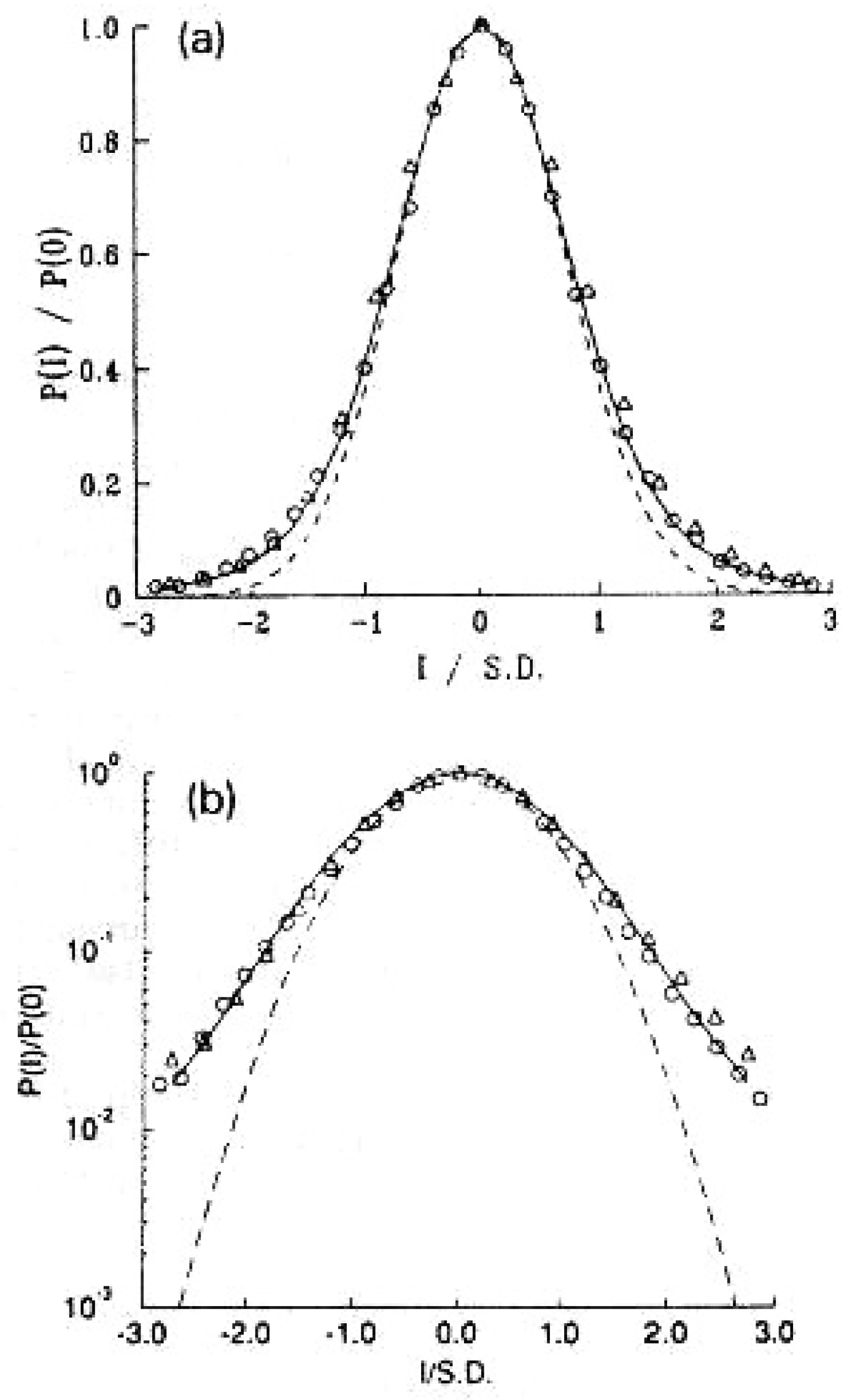
The HRV PSD is determined by the correlations captured in the spectral analysis characterizing temporal ordering of beat-to-beat differences, I ( n ) = B ( n + 1 ) B ( n ) , where B ( n ) denotes the length of the time interval for the beat number n. Peng et al. [36] graphed the histogram for the differences in the beat-to-beat intervals I ( n ) and found that this is a stationary Lévy process such as [given in Appendix 7.2] shown in Figure 1. It was determined by them that the B ( n ) are anti-correlated for typical healthy individuals using a random walk model. Correspondingly, this correlation was determined to vanish in patients with heart disease but its vanishing was determined to not influence the PDF of the heart beat increments. Both healthy and diseased individuals were described by Lévy stable PDFs without being able to statistically distinguish between them thereby demonstrating that the distribution of inter-beat fluctuations { I ( n ) } does not uniquely characterize healthy HRV time series since it is their time ordering that has accurately captured the fractal nature of the beat-to-beat interval time series.
The time series analysis of HRV performed by Peng et al. [36] indicated that the statistics of the fluctuations in the HRV are Lévy stable which they obtained using a random walk model. This observation refuted the widely held belief that cardiac activity observed in healthy individuals is Normal in a statistical sense. They demonstrated that rather than following a bell-shaped curve of the Gaussian type the statistics of heart beat intervals are characterized by heavy tails, see Figure 1, signifying that deviations from the average are far more likely than expected from a Gaussian process as visually highlighted in Figure 1b. This is the zeroith order FOC model (FOCM-0) since it implies the need for Lévy statistics thereby entailing the FOC but that calculus was not used in its empirical determination by Peng et al.
However such functional dependence shares an undesirable property which is also observed in the HRV PSD that being a diverging second moment. This divergence implies that the heart beats of all healthy individuals would be asymptotically unstable, a conclusion that is medically unacceptable for a healthy HRV time series. A number of suggestions have been made to overcome this unrealistic divergence of the HRV which we subsequenty touch on. Herein we adopt some ideas from control theory adapted to the fractional calculus as a means of resolving the objections raised with regard to these early suggestions.

3. Theoretical Lévy statistics for HRV: FOCM-1

The empirical Lévy PDF was at the center of the analysis of HRV time series conducted by Peng et al. [36] and which suggested to us [56] that the FOC might provide a strategy for going beyond the random walk interpretation of the HRV time series proposed by these groundbreaking investigators. Instead West and Trualska [56] introduced a Langevin equation to replace the random walk argument of Peng et al. to determine the fractional form of the diffusion equation used to find the Lévy statistics:
d I ( t ) d t = ξ t .
Here ξ t is the non-Gaussian random force produced by the autonomous nervous system (ANS) which manifests the conflct between the time series produced by the sympathetic (increases HR) and that produced by the parasympathetic (decreases HR) which was empirically determined to be an infinitely divisible IPL distribution using characteristic functions.
The probability that the dynamic variable I ( t ) lies in the phase space interval ( I , I + d I ) at time t is P ( I , t ) d I , where the PDF is defined as a solution to a fractal-order Fokker-Planck equation (FOFPE) [52]:
P I , t t = K β I β P I , t ,
where we have introduced the symmetric Reisz-Feller fractal-order derivative (FOD) I β · whose Fourier transform is | κ | β with κ the Fourier variable conjugate to the phase space variable I and K β is a ’diffusion’ constant. Equation (4) is a fractional diffusion equation for the evolution for the PDF in the heart beat intervals, whose solution is the Lévy distribution given by the integral [52]:
P ( I , t , β ) = 0 d κ π cos κ I exp t K β κ β .
The Lévy PDF given by Eq.(5) agrees with the histograms of the HRV data depicted in Figure 1 for a fixed time, with the Lévy index β = γ = 1.7 and a positive definite diffusiion coefficient K β > 0 . Note that in each case the value for the numerically generated Lévy random force is that obtained for a healthy individual which is provided by the ANS drivers.
The FOFPE is a model FOC equation of evolution assumed to govern the behavior of the PDF for the dynamics of healthy heart rate fluctuations. However its value for the present study lies in its forming the first link in the chain of logic connecting this unsatisfactory model with one which allows for the inclusion of the cardiac control mechanisms which satisfy all our present day modeling concerns.

3.1. FOCM-0 and FOCM-1 Are Both Unacceptable

Peng et al. [36] find that the statistics of healthy and diseased (dilated cardiomyopathy) conditions are the same, that being Lévy stable with index γ = 1.7 , however the spectra for the two cases are quite different. The PSD S p ( f ) is given by the square of the Fourier transform of I ( n ) yielding S p ( f ) 1 / f β , where β = 2 δ 1 and the mean-square level of the interbeat fluctuations increases as n 2 δ . Here again δ = 0.5 corresponds to Brownian motion, so that β = 0 indicates the absence of correlations in the time series I ( n ) (“white noise”). See Table 1 and the discussion of the relations among the scaling indices in Appendix 7.1.
They [36] observed that for a diseased data set that the PSD IPL index β is approximately zero in the low-frequency regime confirming that the I ( n ) are not correlated over long times. On the other hand, they also observed that for the healthy data set the PSD IPL index β is approximately equal to 1 indicating a long-time correlation in the interbeat interval differences. The anti-correlated property of I ( n ) are consistent with a nonlinear feedback system that “kicks” the heart rate away from fluctuation extremes. This tendency operates on a wide range of time scales not on a beat-to-beat basis. The conclusion is that the different scaling pattern must be a consequence of the ordering of the differences, rather than their statistics, which is to say in the correlations produced by the underlying dynamics.
The first step in the logic chain has therefore been the introduction of the IPL fluctuaions in a Langevin equation giving rise to the FFPE Eq.(4) and the Lévy PDF solution given by Eq.(5). This model of the HRV statistics is unacceptable due to the divergence of the second moment in the Lévy model of any phenomena including an HRV time series. However, it does capture what was known at that time which leads to our formulating the next link in the chain of FC modeling logic, which is how to temper the large-scale fluctutions and thereby retain stability of the HRV time series by intoducing a reasonable mechanism to reduce the tails of the Lévy PDF while simultaneously maintaining the proper scaling in the central region of the empirical PDF.

4. Tempering Fluctuations: FOCM-2

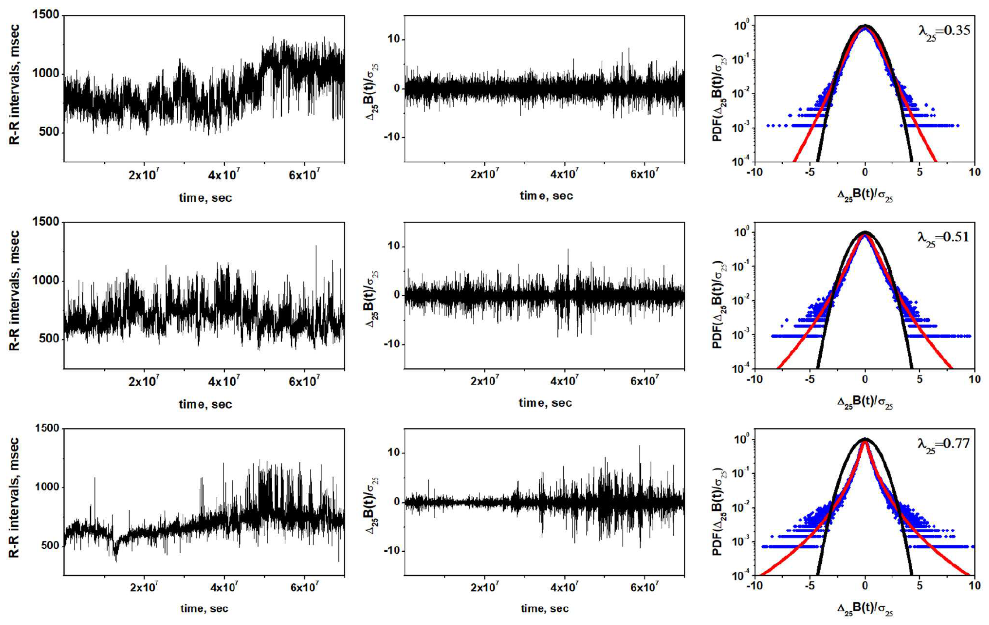
In Figure 2 is depicted a number of representative exemplar datasets of HRV time series for a healthy control group (top row) and two subsequent rows with pathological HRV time series [see Appendix 7.4 for details]. The value of the parameter λ 25 in the upper right hand corner in each of the final panels of the three rows provides a measure of the deviation of the time series of interest from the best Gaussian fit to the depicted data [6]. Scanning down the figure it is clear that the larger the value of λ 25 the less the tails of the fitted Lévy PDFs conform to those required for healthy functon. Notice that the red curve in the bottom row flares out to ± 10 standard deviations indicating that this person’s heart spends a large fraction of its time in the off or relaxed position.
We hypothesize a physiologic feedback mechanism that exponentially suppresses very large fluctuations at both postive and negative extremes. The feedback mechanism in FOCM-2 is equivalent to the so-called tempering mechanism previously used by [22] to explain the three PDFs characterizing a cohort group of 670 post-AMI (acute myocardium infarction) using 24-hour Holter monitor data to construct heartbeat interval data from the HRV time series depicted in the figure from [22]. It has been argued that a modified FOFPE yields the tempered Lévy PDF and can be obtained by the direct inclusion of a disspation rate in the Reisz-Feller fractal derivative term in Eq.(4) to obtain FOCM-2:
P I , t t = K β ( I + λ ) β P I , t .
The exact solution to this equation is given by an exponentially truncated Lévy PDF, see Section (7.6.1) of [55] for details:
P I , t ; β , λ = e λ I L β I , K β t ,
where L β I , K β t is the Lévy PDF given by Eq.(5). The completely scaled form of the PDF is determined in terms of the probability for the scaled variable I s = I ( K β t ) 1 / β :
P I , t ; β , λ d I = e λ s I s L β I s d I s ,
where we have used the infinite divisibility of the PDF to obtain the exact form of the solution to Eq.(6) given by Eq.(8).

4.1. Why Is FOCM-2 Unacceptable?

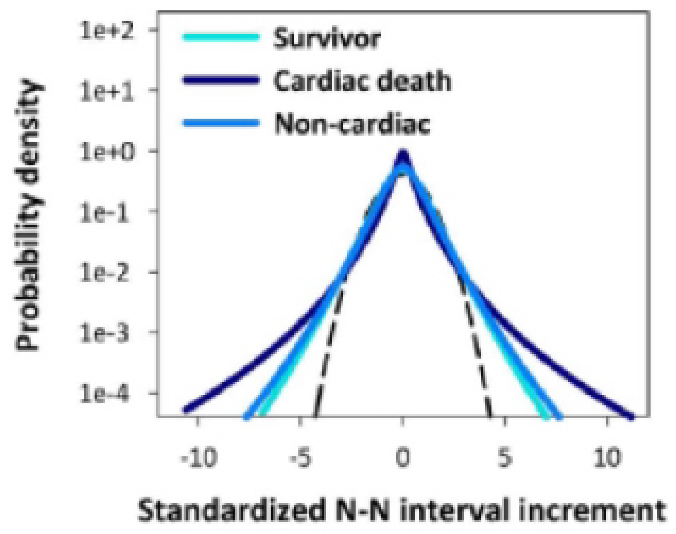
Figure 3 depicts the empirical result that those surviving and those that have died in the cohort group of 670 patients due to non-cardiac causes have essentially the same distribution due to the values of the hypothesized cardiac control mechanisms which are significantly larger than those that suffer cardiac deaths. Said simply, those that suffer cardiac deaths do so because the control mechanism that suppresses the larger fluctuations has failed. This elegant mathematical result has a fatal drawback which is, of course, that the physiological source mechanism for the dissipation parameter λ 25 in Eq.(6) resides in the model ANS, if it existed (it does not), and not in the model sinoatrial pacemaker cell. FOCM-2 would be the preferred model if the fluctuations and dissipation were generated by the same process but that is not the case here.
We need a control mechanism that "kicks" the heart rate fluctuations away from its extremes as so colorfully explained by Peng et al. [36] whereas FOCM-2 suppresses the extreme fluctuations before they have a chance to disrupt the HRV time series which is not the situation observed by Peng et. al. and for that reason the model must be rejected in favor of an explict nonlinear control process that can explain equally well the results recorded in both Figure 2 and Figure 3.

5. HRV Control Hypothesis: FOCM-3

As the third and last step in our logic chain for the HRV example we hypothesize the existence of cardiovascular control mechanisms which leads to a tempered Lévy PDF characterizing CETS in healthy individuals using a FOC model. This control mechanism suppresses the larger fluctuations of those in the Lévy PDF tail which persists in various cardiac disorders. The pathophysiology of the HRV PDF being Lévy stable therefore results from this physiological control process suppressing of the extreme fluctuations in the HRV and differs from the exponential tempering of the Lévy PDF found in the literature, e.g., see [28,54,56]. We here again model the HRV time series to be determined by a nonlinear Langevin equation, where the nonlinear deterministic force corresponds to the control process acting to suppress the fluctuations exceeding a given physiological level beyond which the ON becomes unstable. The corresponding Fokker-Planck equation takes on a fractional form, whose steady-state solution is a tempered Lévy distribution. West and Turalska [56] captured the dynamics of cardiovascular-like systems in the framework of a FOC and their results are adapted to the needs of the present FOC model.
The HRV time series is a consequence of numerous control mechanisms that shape the cardiac activity and the most fundamental component of the HRV is formed by the firing of the pacemaker cells in the heart’s sinoatrial node [21]. This periodic action is continuously modulated by two competing branches of the ANS with sympathetic stimulation increasing the firing rate and parasympathetic action decreasing that rate [17,18,36] as stated earlier. Now we address the significance of the heart’s primary pacemaker, the sinoatrial node, in controlling the balance in the competition between these two branches of the ANS. The importance of the response of the sinoatrial node to autonomic signaling to heart rate and HRV has been emphasized by [56,62].
IPL spectra have been observed in a number of dynamical systems having chaotic solutions, see, for example, Reichl [38]. Goldberger and West [17] suggested that the observed PSD of the HRV may be a consequence of such dynamics and that one may interpret the modifications in the IPL PSD as being indicative of pathology and therefore may be of diagnostic and prognostic value. Loss of complexity in the HRV has already been described in numerous settings, including multiple sclerosis [35], diabetes mellitus with neuropathy [38], fetal distress [26], bed-rest deconditioning [16], aging [47] and in certain patients at risk for sudden cardiac death [14,34]. Presumably, the more severe pathologies will be associated with the greatest loss of spectral power which have been referred to as losses of spectral reserve [15,17]
West and Turalska [56] point out that there is no á priorireason to restrict the control analysis of HRV dynamics to linear negative feedback. In physical systems the fluctuations and linear dissipation have a common origin and consequently are tied together by Einstein’s fluctuation-dissipation theorem [10] which implies an underlyiing linear response mecanism. In the life sciences, however, the significant random force and dominant determinisic force that appear together in the Langevin equation have different sources and the determinisitc feedback must be adaptive to regulate the random force while simultaneously responding to it. They [56] assumed in the case of HRV time series that the deterministic force F ( I ) is generated by the collective behavior of the sinoatrial pacemaker cells and the sum of the competing contributions from the sympathetic and parasympathtic components of the ANS is ξ ( t ) being written as afractal-order nonlinear Langevin equation (FONLE):
d I ( t ) d t = F ( I ) + ξ ( t ) .
This argument was used to determine the FOFPE which when the deterministic force is taken to be linear the solution to the fractal partial differential equation was determined by West and Seshadri [50] to yield a Lévy PDF solution as discussed with regard to the FOCM-1.
A generic version of Eq. (9) was analyzed by Chechkin et al. [8] wherein the deterministic term was given by the nonlinear force written as F ( I ) = λ ( I ) I :
d I d t = λ ( I ) I + ξ ( t ) ,
Equation (10) reduces to the linear Langevin equation of the last section with λ 0 λ ( 0 ) and ξ t is again assumed to be a renewal process with index β [13]. In general the feedback term is a polynomial, but [56] restricted the analysis to the highest-order non-vanishing term, since this term asymptotically dominates the control process and wrote λ I λ 0 + λ 2 n I 2 n . But here this replacement is considered to be unsatisfactory because the nonlinear form of the dissipation coeffficient λ I was selected soley to overcome the divergence of the variance I 2 .
Herein we acknowledge the weakness of the model put forward in [56] and replace the determinstic force used therein, in keeping with the overall strategy of learning from previous defects in modeling the FONLE. The error in the earlier work is corrected for the present model by replacing the deterministic force in the FONLE by:
F ( I ) λ 0 + λ ν I 2 ν I
where the power-law index ν can herein be non-integer and the absolute value of I insures that the deterministic force is symmetric. Note that Eq.(11) is equivalent to our replacement of I 2 used in [56] with I 2 ν = I 2 ν where ν 0 .
The technique presented in the Appendix 7.2 enables the replacement of the FONLE containing the lowest-order nonlinear term in the sinoarial node dynamics given by Eq.(11) with a corresponding FOFPE that is expressed in the present situation as:
P I , t t = I ( λ 0 + λ ν I 2 ν ) I P ( I , t ) + K β I β P I , t .
Note that this equation is the same ’form’ of FOFPE studied by Chechkin et al. [8] where the ’drift’ term λ 0 I is analogous to the harmonic Ornstein-Uhlenbeck potential. The next integer-order contribution is 1 I 3 and would be analogous to a quartic potential. It is clear that the quartic potential suppresses the divergent second moment, but the fourth moment still diverges and requires the next-order disspation to quell that divergence.
Of course, we cannot solve the full time-dependent FOFPE given by Eq. (12) in general but it is not necessary to know the exact solution to obtain the information we need to test our control hypothesis. The asymptotic behavior of the steady-state solution is sufficient for that purpose. The asymptotic steady-state solution to the FOFPE is given by setting Eq. (12) to zero and retaining only the lowest-order nonlinear term to obtain:
λ ν I 2 ν + 1 P s s I = K β d d I I P s s I d I I I β 1 .
A formal argument using the ansatz P s s I C / I γ , γ > 0 yields the normalized solution for the approximated steady state to be the IPL PDF (see Appendix 7.2 for details) [8,56]:
P s s I = N γ I γ ; γ = β + 2 ν + 1 ,
where N γ is the normalization constant and the equation is valid for I ± due to symmetry. Here we paraphrase the conclusion reached by Chechkin et al. [8] that for all the values of the power law index greater than the critical value ν > ν c r = 2 β the variance I 2 is finite, and consequently a nonlinearity whose highest power ν exceeds the crucial value ν c r counterbalances the information overload injected by the complexity of the ANS to the information exchange with the sinoatrial node.
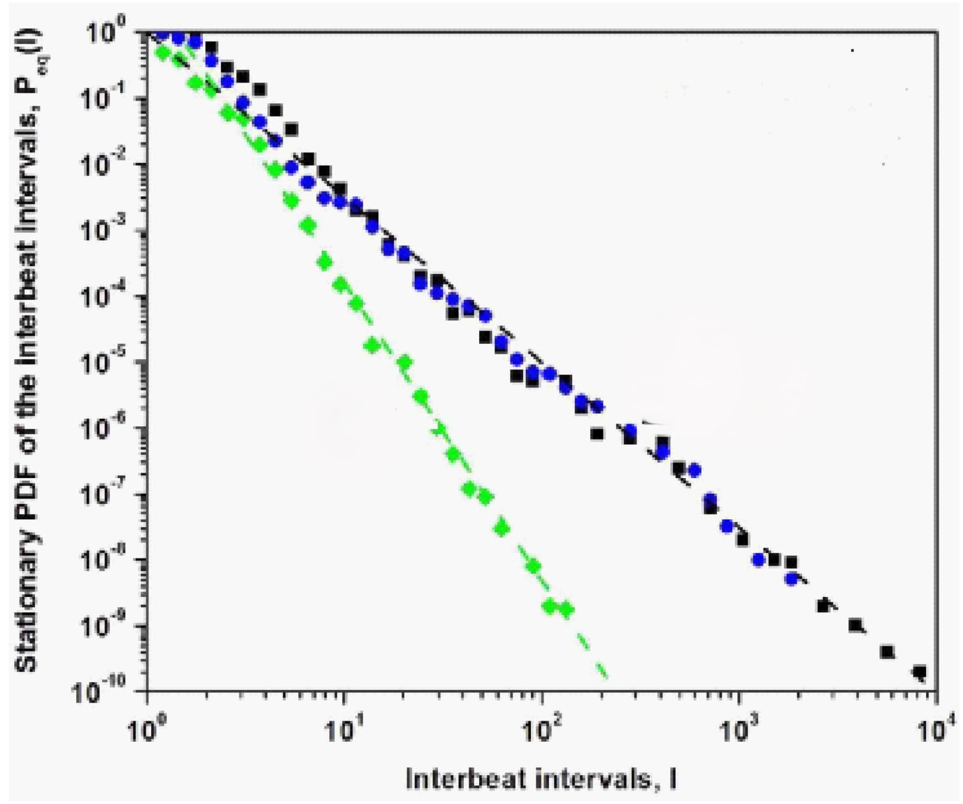
In Figure 4 three steady-state IPL PDFs are calculated using the asymptotic solution to the FOFPE at the two extremes of the interval 2.7 γ 4.7 are shown with two of them being degenerate when ν = 0 . The steady-state scaling index γ of the PDF is fit to the numerical solution of the steady-state FOFPE (see Appendix 7.2). In the numerical simulations with β = 1.7 used to drive the dynamics of the sinoatrial node modeled as a dynamic network near a tipping point. It is clear from Figure 4 that the deterministic force is selected to have the formal steady-sate solution that captures the three IPL forms predicted by the steady-state solution to the FOFPE with either γ = 2.7 with ν = 0 (pathological) or γ = 4.7 with ν = 1 (healthy). It is clear that the extreme values of the control index ν acts like a switch for turning the physiologic control of HRV fluctuations on or off indiating that there is a significant potential range of ν over which clinicians may be able to intervene and restore control of the HRV to an appropriate healthy level.

5.1. Why is FOCM-3 Acceptable?

The model is acceptble because it provides a reasonable separation into healthy and diseased individuals shown in Figure 4 as well as further discriminating between those that have died due to heart disease from those that have passed due to other causes yielding the interesting partitoning into the three groupings of patients recorded in Figure 3.
It is well known that for an IPL index γ 3 the second moment I 2 is finite as a consquence of the central limit theorem holding asymptotically. Consequently, for ν = 1 the statistics of I have a finite second moment asymptotically and the steady-state PDF asymptotically transitions from Lévy stable to Gaussian. This transition explains the result obtained by Kiyono et al. [28] without the need to exponentially temper the random force in the FOLLE, relying solely on the sinoatrial node dynamics to temper the extreme fluctuations resulting from the competition between the two branches of the ANS.

6. Discussion and Conclusions

There are a number of take home lessons to be derived from the presentation starting with never being satisfied with the early FOC models developed to explain a complex process which is not to say don’t publish the argument or the model. But no matter how elegant the mathematics go back to it again and again until you have answered all your questions and those of your colleagues. But most importantly make notes of the changes in your thinking as the levels of FOC modeling unfold. So let us quickly review what we learned at each step of the modeling process presened herein.
The analysis of HRV data by Peng et al. [36] indicated that the statistics of the changes in heart beat intervals are Lévy stable. The Lévy statistics have the property that the second moment of a time series with such statistics diverges consequently implying that the heart beat of every healthy person would be asymptotically unstable. A number of investigators have argued that this instability is readily quenched by introducing a mechanism to dampen the largest fluctuations produced by the Lévy driver thereby producing a tempered Lévy PDF, see e.g. [22,27].
FOCM-0 verified the processing of the empirical HRV time series for the healthy state of variability of the heartbeat intervals as a Lévy PDF but ultimately it is unsatisfactory because the Lévy PDF has an unphysiologic divergence of the second moment. The FOCM-0 is too simple.
The scaling of the statistics for the central or Lévy part of the tempered PDF is the same for both the healthy and CHF patients in Figure 2. Consequently, those that suffer from a serious cardiological condition have greater heart rate variability, but their HRV is certainly less complex than those whose HRV variability is restricted by a nonlinear control process. Thus, interpreting complexity to be proportional to the second moment (variability) in the HRV context is too simplistic.
FOCM-1 was designed to provide a formal mathematical description of the Lévy PDF empirically observed by [36] in FOCM-0. The natural calculus to obtain this PDF is the FOC but the FOFPE given in Eq.(4) requires additional modifications to incorporate the tempering mechanism in the dynamics and thereby avoid the second moment divergence.
The data shown in Figure 2 suggest the use of exponentially tempered Lévy statistics to explain the difference between healthy individuals and CHF patients. The tempering control mechanism would suppress the largest excursions in time, which persist in the severe CHF groups. The pathophysiology of the HRV PDFs being Lévy stable would then be the result of the suppression of a physiological control mechanism as suggested in [54]. However, the form of this earlier hypothesized control mechanism would need to operate at the level of the involuntary nervous system and not be a separate and independent balancing mechanism such as proposed herein and supported by the empirical evidence.
FOMC-2 uses the infinite divisibilty of the PDF to obtain Eq.(6) which has an elegant tempered Lévy PDF solution. However it does not realize the proper control mechanism to supress the heart rate at the extremes, but instead suppresses the extreme flctuations themselves before they can disrupt the HRV time series.
However, there is the additional scaling of the HRV in the tempered Lévy PDF produced by the criticality of the healthy sinoatrial node dynamics. Criticality, as manifest in the nonlinear term in the new FONLE given by Eq.(11), reduces the span of the fluctuations from those that persist in severe CHF condition to those present in more manageable CHF cases. This second scaling, which is produced by the proposed control mechanism, certainly adds to the overall complexity of the process, by introducing a second scaling mechanism. It is the weakening and ultimate loss of this control modeled by the control parameter ν 0 that lifts the restriction on the span of the fluctuations in HRV time series, resulting in certain cardiac pathologies. The source of the physiological control mechanism in the FONLE given by Eq.(11) is based on the sinoatrial node dynamics being poised at criticality [56] and is inserted into Eq.(9) to create the full nonlnear control mechanism in the FOFPE Eq.(12).
They [56] noted further that the sinoatrial node is comprised of a network of interacting pacemaker cells, the collective behavior of which provides insight into critical phase transitions in non-physical networks. The model they chose to mimic the complexity of the sinoatrial node was the Decision Making Model [53] which near criticality reduces Eq.(10) to a cubic Langevin equation, which although qualitatively correct, like the tempered Lévy PDF discussed earlier, errs in quantitative detail for this particular application.
FOCM-3 solved this remaining problem by introducing a nonlinear negative feedback mechanism that is self-regulating and is asymptotically consistent with the hypothesis that “disease is the loss of complexity” made by [17].
Let us use our new-found insight into explaining the three curves in Figure 3. Here we separate the cohort groups into the living and the dead. When the hypothesized control network is on and working properly, i.e., when ν = 1 , the largest fluctuations in the HRV time series are suppressed thereby producing a tempered Lévy PDF. This would account for the survivor curve consisting as it does of only the living. This first cohort group consists of those alive all having ν = 1 and the second cohort group consists of those that are all dead but this latter group can be usefully further subdivided into those that died by extreme cardiovascular malfunction and those that are equally unluckey but their hearts are fine up to the point where they no longer beat, but the cause of death must be sought outside the cardiovascular network. It is this latter subdivsion that accounts for the cardic ( ν = 0 ) and non-cardiac ( ν = 1 ) deaths.
Thus, we may tentatively conclude that the FOC provides a sufficiently general infrastructure to build successively more complex models of real physiological networks as unseen tasks being performed in the background of healthy networks are revealed when they fail to properly respond to the signals from other networks due to illness or injury ( I o I ). This opens the door to a general theory of rehabilitation using crucial events [60]. A correct model of the diagnostic for I o I as in the case of the weakening of the control mechanism ( ν c < 1 ) often suggests how the I o I can be healed through the introduction of an aritificial control mechanism ( ν a < 1 ν c ) to temper the extreme fluctuations such that ν = ν c + ν a 1 thereby restoring the heart’s rehabilitated HRV to a healthy scaling value.

Funding

B.J.W. is retired and conducted the research independent of any funding source.

Data Availability Statement

Data used to support the findings of this study are all available in the open literature.

Conflicts of Interest

The author declares that the research was conducted in the absence of any commercial or financial relationships that could be construed as a potential conflict of interest.

Appendix A. Appendices

Appendix A.1. On Crucial Events (CEs)

We have hypothesized [58] that the ONs making up a NoON such as the human body each generates time series X ( t ) consisting of a seuence of CEs modulated by a mulifractal dimension (MFD) index δ t such that by scaling the time we obtain the scaling relation X ( λ t ) = λ δ ( t ) X ( t ) . Empirically the phenomenon of a sequence of crucial events (CEs) is based on time series consisting of random discrete events with renewal statistics which enable two interacting organ-networks (ONs) to detect and quantify the complexity of the other ON and to minimize the difference in their relative complexity so as to become synchronized. The quantification of complexity is given by the MFD which becomes equal in each ON time series (ONTS) even though they may be operating on largely different time scales, such as the brain, heart and lungs, see [31,32,59] for a discusision of the synchronixaion of the time-depenent scaling index δ t . The discrete events in such time series have been named crucial because they emerge from the nonlinar complex sub-dynamics to determine the efficiency of information exchange among the members of the NoONs.
A crucal event time series (CETS) is generated by a renewal event time series (RETS) with an IPL waiting-time PDF ( Ø ) Ø μ having an IPL index in the domain 1 < μ < 3. Asymptotically, the generated CETS describes an ergodic process for the IPL index μ in the range 2 < μ < 3 with a finite average waiting time. Ergodic is the technical name for statistical processes for which averages taken over long time series are equal to those taken over PDFs. The understanding of complexity in many-body physics is formally understood by assuming the `ergodic hypothesis’ dating back over a century to the time of Boltzmann
The function F ( y ) of the scaled variable y = x / t δ in a scaled PDF in Eq.(A7) is unknown in general but is well known for certain values of the scaling parameter. This generic form of the solution is obtained from an equation of evolution for the PDF that has an α order derivative in time and a β order derivative in space see Eq.(1) such that the solution to thefractal-order diffusion equation (FODE) can be solved using renormalization group theory as shown in FOCM-2 to obtain the scaling PDF with the scaling index δ = α / β [58]. The ordinary diffusion equation has the integer-order indices α = 1 and β = 2 yields the well-known scaling index δ = 1 / 2 in which case the unknown function F ( y ) becomes a Gaussian with the scaled variable y = x / t . Note that the fractal dimension D for this process is obtained from D = 2 δ = 1.5 which is therefore a monofractal process that is completely random, which is to say it is simple diffusion with no memory. Consequently, scaling PDFs with δ 1 / 2 are anomolous in that their fractal dimension and D 1.5 and they contain various forms of memory.
If the anomoly has a completely temporal ( α < 1 ) origin we have for the spatial derivative index β = 2 for a spatially homogeneous process and δ < 1 / 2 thereby producing the fractal dimension D > 1.5 indicating the existence of a memory-like process. The more the scaling index deviates from 1/2 the more the fractal dimension deviates from 1.5 and the stronger the anomoly. If the time deviation is produced by a fractal time series with an IPL waiting-time PDF which when these time intervals are statistically independent of one another constitues a renewal time series. The renewal time series is ergodic for 2 < μ < 3 with a finite average waiting time and is non-ergodic for 1 < μ < 2 with a diverging average waiting time.
Suppose the trajectory X t crosses a known level at a specific time and we want to know how long we must wait to recross that same level. Given that the waiting-time PDF has the IPL form we denote the generic IPL index for the waiting-time PDF μ by the symbol μ D . From the parameter relations in Table 1, it is clear that it is possible to prove that the IPL index is equal to the fractal dimension, so that we obtain [12,59]:
μ D = D = 2 δ ,
which is possible to establish using the probability of crossing and recrossing any fixed value of the diffusion trajectory which has been shown to be a renewal process and is consequenly a CETS.
The PSD S p ( f ) for a CETS is also IPL in terms of the frequency f:
S p ( f ) f β ,
indicating 1 / f variability. This IPL PSD is the Fourier transform of a slowly decaying auto-correlation function indicative of a fractal time series having global or local self-similarity. The IPL indices μ and β are interrelated for the class of fractal time series of interest in medicine such that the fractal dimension given by Eq.(A1) is related to the IPL PDF index defined by Eq.(A2), and the IPL index for the PSD is [58]:
β = 3 μ .
Thus, true 1 / f noise at β = 1 arises only at the boundary μ = 2 between the ergodic and non-ergodic variability domains.
Table1 is copied from West et al. [60] and provides easy reference to all the derived relations among the IPL scaling indices for the PSD index β , the IPL waiting-time PDF index μ and the scaling index δ for the scaled variable X ( t ) as well as the scaled PDF.
Figure A1. In this table we record the scaling index δ from the homogeneous scaling relation for the scaled variable X ( t ) , relating it to the IPL power spectrum index β through the waiting-time PDF ψ ( τ ) IPL index μ . The value μ = 2 is the boundary between the underlying process having a finite ( μ > 2 ) or an infinite ( μ < 2 ) average waiting time and is also the point at which β = 1 where the process is that of true 1 / f noise. Consequently, β and μ are interchangeable measures of complexity. For an ergodic time series such as that determined by the waiting-time inverse power-law index μ increases with decreasing scaling index δ and the fractal dimension increases. Adapted from [31] with permission.
Preprints 118088 g0a1
The work of [1,25] have demonstrated reduced multifractality associated with impaired parasympathetic control and pathological condition of CHF, respectively. This corresponds to a reduction of long-range correlations present in the HRV of healthy individuals, an outcome related to a loss of dynamical properties of the cardiovascular system. The control mechanism introduced herein is presented in terms of a FOFPE given by Eq.(12) which leads to investigations of HRV through its PDF distribution. The FOFPE is a theoretical model that describes the evolution of the PDF of the physiologic process and its solution (when it can be obtained) captures the full dynamics of an ensemble of time series.
The adaptive feedback control process produced by the collective behavior of the pacemaker cells, postulated herein, is physiologically simpler than the exponential tempering suggested earlier [54] and applying Occam’s razor, is the more likely explanation. The nonlinear term is a collective effect within the sinoatrial node dynamics and produces a tempered response to the stochastic excitations. This tempering of the extreme HRV excursions is pathologically suppressed within the severe CHF group. The pathophysiology of the HRV PDF being Lévy stable is then the result of a suppressed control process, which can no longer determine the maximum size of the interbeat intervals, resulting in lossing the control of disease.

Appendix A.2. Scaling Solution to Fractal Kinetic Equation

Zaslavsky et al. [39,63] applied the renormalization group transformation R to the network dynamics such that the scaling properties of the incremental changes are: R : δ x = λ X δ x ; R : δ t = λ T δ t , which apply, after some averaging, to a restricted space-time domain and the scaling parameters are ( λ X ; λ T ). They continue with the observation that the fractal kinetic equation (FKE) given by Eq.(1) is invariant under the renormalization group transformation:
R : D t α P x , t = K β R : D x β P ( x , t )
which implies that the transformed fractal equation satisfies the scaling behavior:,
λ T α D t α P x , t = K β λ X β D x β P ( x , t ) .
The lowest-order renormalization group solution is given by equating the renormalization parameters raised to their respective powers: λ T α = λ X α . The solution to the renormalized FKE is given in terms of the Fourier transform of the PDF, which is the characteristic function ϕ ( k , t ) , expressed in terms of the Mittag-Leffler function E β ( . ) to be:
ϕ k , t = E β K β k β t α .
Consequently, taking the inverse Fourier transform of this characteristic function and expressing the Mittag-Leffler function as an infinte series, after some algebra [55,63], results in the scaling solution for the PDF:
P x λ T α / β , λ T t = P x , t / λ T α / β .
Selecting the ratio of the scaling parameters to be the exponent of the remaining scaling parameter: δ = α / β , and choosing the time scale of interest to reduce the dependence of the PDF on the left side of the equality in Eq.(A6) to be dependent on the single scaled variable x / t δ using λ T = 1 / t , enables us to rewrite Eq.(A6) in the form of the scaling PDF given by
P ( x , t ) = 1 t δ F x t δ .
Thus, the solution to the FKE yields the scaling PDF along with the DEA data processing technique to interpret the datasets from the brain, heart and lungs in the text as CETS with synchronized levels of complexity as measured by their respective multifractal dimensions.

Steady state solution ;

Chechkin et al. [8] argue that the behavior of the steady-state PDF can be determined from an analysis of the contributions to the integral in the fractal deivative in Eq.(12) in the vicinity of the pole:
λ 2 ν I 2 ν + 1 P s s I C β d d I I P s s I d I I I β 1 = 0 .
In particular, the dominant contribution to the integral arises from the region to the left of the pole I = I and consequently the operator may be approximated by the expression shown below. The integral term may be expressed exactly as:
I P s s I d I I I β 1 = I 1 β I P s s I d I 1 I I β 1
so that expanding the numerator and noting:
I P s s I d I 1
yields to the lowest-order approximation to the numerator expansion:
I P s s I d I I I β 1 I 1 β .
Inserting this expression for the integral into Eq.(A8) and taking the derivative yields, after some algebra, the asymptotic symmetric steady-state PDF given by Eq.(14).

Appendix A.3. Diffusion Entropy Analysis (DEA)

In this section we indicate how to determine the empirical IPL scaling indices consistency with the theory presented in the previous section and summarized from the Appendices in [32,60]. This consistency is accomplished using the DEA to process the recorded time series generated by the members of the triad of ONs consisting of the heart, lungs and brain. The main text in the above two papers contains the results of applying this method to the 66 ONs of the triad. The sequential steps in the DEA technique referenced to Figure A2 are:
1.) The raw data of each channel is projected onto the interval [0,1] by normalizing each time series by the total time interval of the dataset thereby enabling the processing of each time series to be directly compared.
2.) Divide the normalized data profile into parallel stripes of size of 0.01 (panel (a), ECG data).
3.) Extract events by defining them as unit amplitude pulses if the signal at that time is in a different stripe with respect to its previous value (panel (b)) and zero if it remains in the same stripe.
4.) Create a diffusion trajectory (panel (c)) using the time series of the extracted events from step 3.
5.) Determine the statistics of a single diffusion trajectory by selecting a window size w and partitioning the diffusion trajectory into many pieces, each starting from an event.
6.) Initiating all the trajectories from an event enables their being shifted to start from a common origin (panel (d)).
7.) Finally, we evaluate the ensemble distribution of histograms at a given time (panel (e)) since the events are statistically independent.
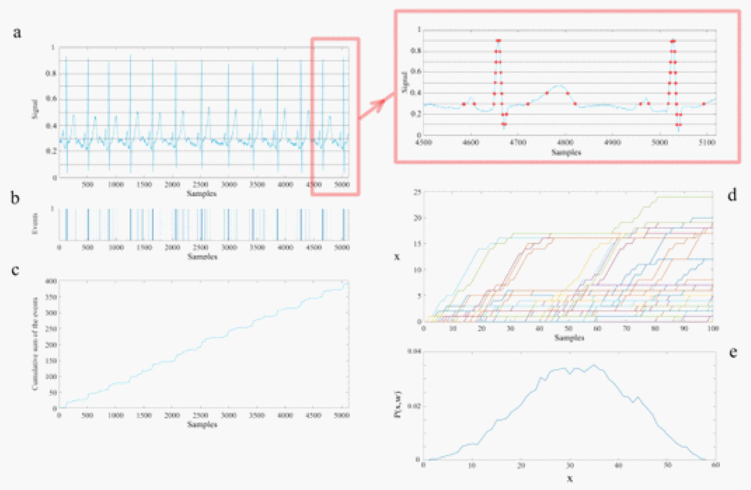
Figure A2. A schematic of the steps for the processing of time series using the technique Diffusion Entropy Analysis. Panel a): The solid curve is the heart rate signal projected onto the interval [0, 1] divided by the stripe size of 0.1, which is magnified in the inset. Note that sharply peaked features in the ECG have a cluster of events in (b), whereas a sloping feature has well-spaced events, see the inset for a visual verification of this explanation. The horizontal lines define the stripes. Panel b): The events (represented as distinct separated unit positive amplitude pulses) are extracted from the passage of the continuous time trace of the ECG from one stripe to another. Panel c): The diffusion trajectory made by the cumulative summation of the events of panel (b). The vertical lines show a selected set of windows with sizes 100 that sliced the diffusion trajectory. Panel d): The partitioned trajectories of panel (c) shifted to initiate each trajectory from a common origin and terminate each after a time w=t, the length of the window. Panel e): The histogram of the position of the trajectories at the end of the windows (to create this histogram 60 sec of data and stripe width of 0.01 which were the DEA parameters used in the data processing.) Taken from [59] with permission.
Preprints 118088 g0a2
To make the statistics of the single time series diffusion trajectory correspond to that done in the DEA processing of the data we pick a window w = t starting from a common origin event (panel d) and evaluate the distribution of trajectories at time t (panel e). Denoting the time-dependence PDF for different windows as P ( x , w ) we can define the SW-entropy as:
S ( w ) = d x P ( x , w ) log 2 P ( x , w ) .
Assuming that P ( x , w ) is the PDF corresponding to window size w we can define diffusion entropy using the SW-entropy as being the information contained in the time series. Using the scaling PDF, without knowing the F ( . ) PDF, the deviation of the SW-entropy from its reference state defined by the unknown function is:
Δ S ( w ) = S ( w ) S r e f = δ log 2 w .
Consequently, if a graph of the SW-entropy for an empirical process versus the logarithm of the time yields a straight line we interpret the positive slope to be the scaling index δ as done in the main text.
Healthy living network hosts healthy ONs by maintaining equal strength in transferring information among ONs in a NoONs but gives rise to time series whose mutifractal fluctuations contain control information that guides both the internal behavior in intra-ON and external information exchange during inter-ONs within the NoONs. In fact, the health of the human body is determined by the multifractal dimensions (MFDs) D j ( t ) or equivalently by the scaling indices δ j ( t ) due to the generic relation between the two quantities: D j ( t ) = 2 δ j ( t ) . The scaling index has the ideal value of 1 as the condition for health of the human body. It is a singular condition corresponding to the largest possible scaling and has been used in the analysis of time series as a diagnostic indicator separating patients who have congestive heart failure from those that are healthy [4,5].

Appendix A.4. Non-Gaussian Index

The analysis of non-Gaussianity of HRV starts from integrating and detrending (third order polynomial for the trend was used herein) R-R interval time series [27,28]. After the detrending procedure heart rate increments at scale s are defined as Δ s B ( t ) = B * ( t + s ) B * ( t ) , where B * ( t ) is a deviation of the HRV from the polynomial trend. Then the PDF of differences Δ s B ( t ) normalized by the SD is evaluated. Finally, the non-Gaussianity index λ s is estimated as:,
λ s = 2 q q 2 ln π Δ s B q 2 q / 2 ln Γ 1 + q 2 ,
where | δ s B | q denotes an estimated value of the q th order absolute moment of | Δ s B | . Following [22] we calculate λ s based on the 1/4-th order moment ( q = 0.25 )and we set the scale s at 25 s . The parameter λ s was originallyintroduced as a parameter of log-normal cascade model describing non-Gaussian distributions in the study of intermittency of hydrodynamic turbulence [6]:
P λ , σ 0 x = 0 d ln σ 2 π λ exp ln 2 σ / σ 0 2 λ 2 × 1 2 π σ exp x 2 2 σ 2 .
The value of λ s close to zero corresponds to a PDF close to a Gaussian distribution, while a larger value of λ s means that the observed PDF has fatter tails and a sharper peak in comparison with the Gaussian distribution.
The values (mean SD) of listed HRV indices for the group of healthy subjects and two groups of patients with CHF are presented in Figure 2. All indices overlap with values reported in literature for comparable datasets [2,22]. In line with previous studies [22], congestive heart failure leads to a decrease in values of numerous HRV indices. We observe that the power of the HRV in LF and HF frequency bands, LF/HF ratio or scaling coefficients estimated through DFA are affected by the pathological condition. This corresponds to a change in sympatho-vagal balance, where the CHF leads to a dominance of parasympathetic branch of the ANS. Reduced DFA scaling coefficients reflect diminished correlations present in HRV time series, reflecting reduced complexity of cardiovascular control mechanisms

References

  1. LA Amaral, PC Ivanov, N Aoyagi, I Hidaka, S Tomono, AL Goldberger, et al. "Behavioral-independent features of complex heartbeat dynamics", Phys. Rev. Lett. 86, 6026–6029 (2001). [CrossRef]
  2. F Beckers, B Verheyden and A Aubert. "Aging and nonlinear heart rate control in a healthy population", Am. J. Physiol. Heart Circ. Physiol. 290, H2560–H2570 (2006). [CrossRef]
  3. GE Billman, "Heart rate variability – a historical perspective", Front. Physiol.|Clin. & Trans. Physiol.2(86), 1-86 (2011). [CrossRef]
  4. G Bohara, D Lambert, BJ West and P Grigolini, “Crucial events, randomness, and multifractality,” Physical Review E 96, 062216 (2017).
  5. G Bohara, BJ West and P Grigolini, “Bridging waves and crucial events in the dynamics of the brain,” Frontier in Physiology 9, 1174 (2018).
  6. B Castaing, Y Gagne, and F Hopfinger, "Velocity probability density functions of high Reynolds-number turbulence", Phys. D 46, 177–200, (1990). [CrossRef]
  7. D Chalmers. The Conscious Mind. New York: Oxford University Press. (1996).
  8. A Chechkin, V Gonchar, J Klafter and R Metzler. "Natural cutoff in Lévy flights caused by dissipative nonlinearity", Phys. Rev. E 72:010101 (2005). [CrossRef]
  9. S Crowe, K Cresswell, A Robertson, et al. "The case study approach", BMC Med Res Methodol 11, 100 (2011). [CrossRef]
  10. A Einstein, "Über die von der molekularkinetischen Theorie der Wärme geforderte Bewegung von in ruhenden Flüssigkeiten suspendierten Teilchen",Annalen der Physik 322 (8): 549–560 (1905).
  11. R Failla, P Grigolini, M Ignaccolo, and A Schwettman, "Random growth of interfaces as a subordination process", Phys. Rev. E 70, 010101 (R) (2004).
  12. FJ Feder. Fractals, Plenum Press: New York, NY (1988).
  13. W Feller. An Introduction to Probability Theory and Its Applications, Vol. II, 2nd Printing,John Wiley & Sons. New York, NY (1966).
  14. AL Goldberger, L Findley, MJ Blackburn and AJ Mandell, “Nonliear dynamics of heart failure: implications of long-wavelength cardiopulmonary osciallations”, Am. Heart J. 107, 612-615 (1984).
  15. AL Goldberger, V Bhargava, BJ West and AJ Mandell, “On a mechanism of cardiac electrical stability: the fractal hypothesis”, Biophys. J. 48, 525-528 (1985).
  16. AL Goldberger, D Goldwater, and V Bhargava, “Atrophine unmasks bed-rest deconditioning effect in healthy men: a spectral analysis of cardiac interbeat intervals”, J. Appl. Physiol. 61, 1843-1848 (1986).
  17. AL Goldberger and BJ West, "Fractals: a contemporary mathematical concept with applications to physiology and medicine", Yale J. Biol. Med. 60, 104–119 (1987).
  18. AL Goldberger, D Rigney and BJ West, "Chaos and fractals in human physiology", Sci. Am. 262, 42–49 (1990). [CrossRef]
  19. AL Goldberger. "Giles f. Filley lecture. Complex systems", Proc. Am. Thorac. Soc.3, 467–471 (2006). [CrossRef]
  20. S Guzzetti, S Mezzetti, R Magatelli, A Porta, G De Angelis, G Rovelli, and A Malliani, "Linear and non-linear 24 h heart rate variability in chronic heart failure",Autonomic Neuroscience 86(1-2), 114-119 (2000). [CrossRef]
  21. H Hall. Guyton and Hall Textbook of Medical Physiology, 13th Edn. Philadelphia, PA: Elsevier (2016).
  22. J Hayano, K Kiyono, Z Struzik, Y Yamamoto, E Watanabe, et al. "Increased non-Gaussianity of heart rate variability predicts cardiac mortality after an acute myocardial infraction", Front. Physiol. 2:65. (2011). [CrossRef]
  23. H Huikuri. "Heart rate variability in coronary artery disease". J. Intern.Med. 237, 349–357 (1995). [CrossRef]
  24. N Iyengar, C Peng, R Morin, A Goldberger and L Lipsitz,"Age-related alterations in the fractal scaling of cardiac interbeat interval dynamics".Am. J. Physiol. Regul. Integr. Comp. Physiol. 271, R1078–R1084 (1996). [CrossRef]
  25. PC Ivanov, LAN Amaral, AL Goldberger, S Havlin, MG Rosenblum, ZR Struzik and HE Stanley, "Multifractality in human heartbeat dynamics", Nature 399, 461–465 (1999).
  26. V Kariniemi and P Ammälä, “Short-term variability of fetal heart rate during pregnancies with normal and insufficient placental function”, Am. J. Obster. Gynecol. 139, 33-37 (1981).
  27. K Kiyono, Z Struzik, N Aoyagi, S Sakata, J Hayano and Y Yamamoto. "Critical scale invariance in a healthy human heart raté", Phys. Rev. Lett. 93:178103 (2004). [CrossRef]
  28. K Kiyono, Z Struzik, N Aoyagi and Y Yamamoto. "Multiscale probability density function analysis: non-Gaussian and scale-invariant fluctuations of healthy human heart rate", IEEE Trans. Biomed. Eng.53, 95–102 (2006). [CrossRef]
  29. R Kleiger, J Miller, J Bigger and A Moss. "Decreased heart rate variability and its association with increased mortality after acute myocardial infarction",Am. J. Cardiol. 59, 256–262 (1987). [CrossRef]
  30. arXiv:2406.16117v1 (2024).NM MacKay, "Non-equilibrium Noise in V-shaped, Linear Well Profiles", arXiv:2406.16117v1 (2024).
  31. K Mahmoodi, SE Kerick, P Grigolini, PJ Franaszczuk, and BJ West, ”Complexity synchronization: a measure of interaction between the brain, heart and lungs”, Sci. Rep. 13, 11433 (2023).
  32. K Mahmoodi, SE Kerick, P Grigolini, PJ Franaszczuk, and BJ West, "Temporal complexity measure of reaction time series: Operational versus event time",Brain and Behavior13(7): e3069 (2023).
  33. BB Mandelbrot, “1/f noises and the infrared catastrophe”, IEEE Comm. Conv., Boulder, CO (1965).
  34. GA Myers, GJ Martin, NM Magrid et al. “Power spectral analysis of heart rate variability in sudden cardiac death: comparison to other methods”, IEEE Trans. Biomed. Eng. 33, 1149-1156 (1986).
  35. B Neubauer and HJG Gundersen, “Analysis of heart rate variations in patients with multiple sclerosis. A simple measure of autonomic disturbances using an ordinary ECG”, J. Neurol. Neuosug. Psychiatry41, 417-419 (1978).
  36. C-K Peng, J Mietus, JM Hausdorff, S Havlin, HE Stanley and AL Goldberger, "Long-range anticorrelations and non-Gaussian behavior of the heartbeat", Phys. Rev. Lett. 70, 1343-46 (1993).
  37. M Rahman, "Navigating the landscape of research paradigms: An overview and critique", Inter. J. of Ed. Studies 6(1), 1-18 (2023). [CrossRef]
  38. LE Reichl, The Transition to Chaos, Springer, New York (1992).
  39. AI Sachev and GM Zaslavsky, "Fractiomal kinetic equation: Solutions and applications", Chaos7, 753-764 (1997).
  40. M Shlesinger and BJ West. "Complex fractal dimension of the bronchial tree", Phys. Rev. Lett. 67, 2106–2108 (1991). [CrossRef]
  41. A Smolyak, O Levy, I Vodenska, S Buldyrev and S Havlin. "Mitigation of cascading failures in complex networks", Science Reports/natureresearch10,16124 (2020).
  42. RE Stake. The art of case study research. Sage Publications Ltd. London. (1995).
  43. P Stein, P Domitrovich, N Hui, P Rautaharju and J Gottdiener. "Sometimes higher heart rate variability is not better heart rate variability: results of graphical and nonlinear analyses". J. Cardiovasc. Electrophysiol.16,954–959 (2005). [CrossRef]
  44. Z Struzik, K Kiyono,J Hayano, E Watanabe and Y Yamamoto. "Increased heteroscedasticity of heart rate in fatal heart failure". EPL82:28005 (2008). [CrossRef]
  45. Task Force of the European Society of Cardiology and the North American Society of Pacing and Electrophysiology. "Heart rate variability: standards of measurement, physiological interpretation and clinical use". Circulation 93,1043–1065 (1996). [CrossRef]
  46. LD Valdez, L Shekhtman, CE La Rocca, X Zhang, SV Buldyrev, PA Trunfio, LA Braunstein, S Havlin. "Cascading Failures in Complex Networks", Journal of Complex Networks8(2),1-25 (2020). [CrossRef]
  47. JL Waddington, MJ MacCulloch and JE Sambrooks, “Resting heartrate variability in man declines with age”, Experientia 35, 1197-1198 (1979).
  48. ER Weibel, "Fractal geometry: a design principle for living organisms", American Journal of Physiology-Lung Cellular and Molecular Physiology261(6): (1991). [CrossRef]
  49. ER Weibel, Symmorphosis: On Form and Function in Shaping Life, Harvard University Press, Cambridge, MA (2000).
  50. BJ West and V Seshadri. "Linear systems with Lévy fluctuations". Phys. A 113, 203–216 (1982). [CrossRef]
  51. BJ West and P Grigolini, Complex Webs: Anticipating the Improbable, Cambridge University Press, Cambridge, MA (2011).
  52. BJ West. Fractal Physiology and Chaos in Medicine. Hackensack, NJ:World Scientific (2013).
  53. BJ West, M Turalska and P Grigolini. Networks of Echoes: Imitation, Innovation and Invisible Leaders. New York, NY: Springer (2013).
  54. BJ West. "A mathematics for medicine: the network effect". Front. Physiol.| Fractal Physio. 5:456, (2014). [CrossRef]
  55. BJ West, Fractional Calculus View of Complexity: Tomorrow’s Science, see Section 7.6.1 Truncated Lévy Process, CRC Press, (2016).
  56. BJ West and M Turalska, "Hypothetical control of heart rate variability", Frontiers in Physiogy|Fractal Physiolgy10:1078,1-9 (2019).
  57. BJ West, K Mahmoodi, and P Grigolini, Empirical paradox, complexity thinking and generating new kinds of knowledge,Cambridge Scholars Publishing,UK (2019).
  58. BJ West and P. Grigolini, Crucial Events: Why are Catastrophies Never Expected?,World Scientific, Singapore (2021).
  59. BJ West, P Grigolini and M. Bologna. Crucial Event Rehabiliation Therapy: Multifractal Medicine, Springer International Pub. (2023).
  60. BJ West, P Grigolini, SE Kerick, PJ Franaszczuk and K Mahmoodi, "Complexity Synchronization of Organ Networks", Entropy 25, 1393-1412 (2023). [CrossRef]
  61. Factals in Biology and Medicine: Volume I, TF Nonnenmacher, SA Losa and ER Weibel Eds, Birkhäuser, Boston(1993); Volume II, SA Losa, D Merlini, TF Nonnenmacher and ER Weibel Eds, Birkhäuser, Boston (1998); Volume III, SA Losa, D Merlini, TF Nonnenmacher and ER Weibel Eds, Birkhäuser, Boston (2002); Volume IV, SA Losa, D Merlini, TF Nonnenmacher and ER Weibel Eds, Birkhäuser, Boston (2005)
  62. Y Yaniv, A Lyaskov and E Lakatta . "The fractal-like complexity of heart rate variability beyond neurotranmitters and autonomic receptors: signaling.intrinsic to sinoatrial node pacemaker cells". Cardiovasc. Pharm. Open Access.2:111 (2013). [CrossRef]
  63. GM Zaslavsky, "Chaos, fractional kinetics, and anomalus transport", Phys. Rept.371, 461 (2002).
1
The terminology ’fractal calculus’ is used throughout to emphasize that the fact that the fractal descriptor means that ’fractal geometry’ and ’fractal statistics’ are vastly different from the usual terms of geometry and statisitics. So too is the ’fractal calculus’ (FOC) remarkably different from the integer-order calculus (IOC) and the integer-order differential equations (IODE).
2
Chalmers [7] coined the term ’hard problem of consciousness’ to distinguish the totality of consciosness from the easy poblems that are amenable to reductive logic . Herein we classify nearly every fundamental problem remaing in science as a ’hard’ problem in the sence that they typically arise out of empirical paradox [57].
Figure 1. The histogram resulting from the diffusion equation in I for healthy (circles) and diseased (triangles) subjects where P ( I ) d I is the probability of finding an interbeat increment in the phase space range [ I , I + Δ I ] . To facilitate comparison, we first subtract the mean from the variable I and divide the difference by the standard deviation of the data and rescale the probability with P ( 0 ) . The Lévy stable PDF’s index β is related to the IPL exponent describing the PDF for large values of the variable, while the width of the distribution is characterized by b (see text). Both histograms are well fit by a Lévy stable distribution with β = 1.7 (solid line). The dashed line is a Gaussian distribution fit to the data and is shown for comparison purposes only. Similar fits were obtained for 8 of the 10 normal subjects with heart disease. The slow decay of Lévy stable PDFs for large increment values may be of physiological importance and relate to the dynamics of the system: (a) linear-linear scale; (b) log-linear scale . Adapted from Peng et al. [36] with permission.
Preprints 118088 g001
Figure 2. Representative examples of the non-Gaussianity index analysis [see Appendix 7.4] of the HRV in a healthy individual (Top row), CHF patient of class I, II, III (Middle row), and CHF patient of class III, IV (Bottom row). Left column shows time series of inter-beat intervals, middle column displays corresponding time series of standardized [ I Z = ( I - I ) / σ ( I ) ] heart rate increments, with the mean I and standard deviation σ ( I ) . Right column shows standardized PDFs of heart rate increments. Estimated values of the non-Gaussianity index λ 25 are shown in each PDF panel. In a solid red line is shown the PDF approximated by the non-Gaussian model. From [56] with permission.
Preprints 118088 g002
Figure 3. Three curves characteriing the fates of 670 individuals in a study where there were those that survived and those that died. The distribution of those that died of non-cardiac related causes essentially overlaps those that survived. The much broader distribution are those that died of cardiac related causes. The hypothetical control model in the text explains this effect. Adapted from [55] with permission.
Preprints 118088 g003
Figure 4. The numerical integration of Eq.(12) is used to determine the steady- state PDF with the empirical Lévy index = 1.7. The computational results are fit extremely well by the analytic steady-state IPL PDF given by Eq.(14) with IPL index γ = β + 2 ν + 1 for v = 0 : λ 0 = λ ν = 0 = 0 (black squares); λ 0 = 1 , λ ν = 0 = 0 (blue circles): and for v = 0 : λ 0 = 1.0 , λ 1 = 0.1 (green diamonds). The dashed curves denote the analtic results where the healthy individual v = 1 has control index γ = 4.7 (green dashed line) and a person with totally inoperable control index v = 0 is γ = 2.7 (black dashed line). Note the modest deviation in the numerical calculation away from the IPL due to the linear dissipation. Adapted from [56] with permission.
Preprints 118088 g004
Disclaimer/Publisher’s Note: The statements, opinions and data contained in all publications are solely those of the individual author(s) and contributor(s) and not of MDPI and/or the editor(s). MDPI and/or the editor(s) disclaim responsibility for any injury to people or property resulting from any ideas, methods, instructions or products referred to in the content.
Copyright: This open access article is published under a Creative Commons CC BY 4.0 license, which permit the free download, distribution, and reuse, provided that the author and preprint are cited in any reuse.
Prerpints.org logo

Preprints.org is a free preprint server supported by MDPI in Basel, Switzerland.

Subscribe

© 2024 MDPI (Basel, Switzerland) unless otherwise stated