
Submitted:
13 September 2024
Posted:
14 September 2024
You are already at the latest version
Abstract
The land use land cover (LULC) map is extensively employed for different purposes. The LULC maps provided by the Portuguese National Geographic Information System (SNIG) are not ideal for continuous assessment and regular scrutiny. Machine learning (ML) algorithms applied in remote sensing (RS) data has been proven effective in image classification, object detection, and semantic segmentation. Previous studies have shown that Random Forest (RF) and Support Vector Machine (SVM) consistently achieved high accuracy for land classification. In this study, the application of RF and SVM classifiers, and object-based (OBIA) and pixel-based (PBIA) approaches with Sentinel-2A imagery was evaluated using Google Earth Engine (GEE) platform for land cover classification of a burned area in the Serra da Estrela Natural Park (PNSE), Portugal. This aimed to detect the land cover change and closely observe the burned area and vegetation recovery after the 2022 wildfire. The combination of RF and OBIA achieved the highest accuracy in all evaluation metrics. At the same time, a comparison with the Normalized Difference Vegetation Index (NDVI) map and Conjunctural Land Occupation Map (COSc) of 2023 year indicated that the SVM and PBIA map resembled the maps better.
Keywords:
Machine Learning
; Land cover classification
; Object-based image analysis
; Pixel-based image analysis
; Random Forest
; Support Vector Machine
1. Introduction
Post-wildfire land cover change affects the ecosystem dynamics, biodiversity system, and ecological processes [1,2]. According to the European Commission, land cover indicates “the visible surface of land on Earth (e.g. crops, grass, water, broad-leaved, forest or built-up area)” [3]. Thus, land cover plays a key role in environmental conditions in multiple ways [4]. Several studies have proved that fire events change soil characteristics, which increase runoff and erosion risk [5,6,7], plant diversity [8,9,10], habitat and species composition [11,12,13], water quality [14,15,16], climate [17,18,19], and carbon storage [20,21]. Detecting the land cover change during a wildfire is critical, as it enables authorities to develop prompt disaster management strategies to prevent fatalities caused by landslides and flash floods following a wildfire [22]. Furthermore, periodic assessments scrutinizing burned area recovery and vegetation dynamics after a wildfire provide valuable information for land management and biodiversity recovery monitoring.
According to Copernicus, Portugal is one of the countries most vulnerable to wildfire in the European Union [23]. More than 200 forest fires happened annually in Portugal from 2013 to 2022. Portugal experienced the worst drought in 2017 since 1931, which caused 408 wildfires and involved 563,532 ha of burned area [24,25]. The Serra da Estrela Natural Park (PNSE), the largest protected area in Portugal, experienced the most significant fire since 1975 [26], which involved a burned area of 21,942 ha in 2022 [27]. This study focused on the major burned area in a wildfire that started on 6 August 2022 and ended on 2 September 2022 in PNSE [27]. The fire spread beyond the PNSE to Estrela Geopark. As a recognized Biogenetic Reserve and Geopark [28], the impacts of the large burned area post-wildfire 2022 in the PNSE are concerning. Close monitoring of post-wildfire burned area recovery and vegetation dynamics to observe the ecosystem dynamics and plan for disaster management is imperative.
The open data on land use and land cover (LULC) in Portugal is publicly available in vector format at a scale of 1:25,000 for Land Use and Occupation Map (COS), and in raster format with 10 m pixels for Conjunctural Land Occupation Map (COSc) from the National Geographic Information System (SNIG) [29]. LULC maps are widely used by various stakeholders for research, analysis, planning, and monitoring purposes [31,32,33]. However, continuous assessment and regular scrutiny of the land cover change are not achievable even with the annual update of the COSc [29].
Researchers have been exploring the integration of machine learning (ML) algorithms and remote sensing (RS) data since the late 1990s [34]. It has proven effective in image classification, object detection, and semantic segmentation since the 2010s [35,36,37]. More recently, the integration of ML algorithms and RS data has been widely applied to convert satellite imagery into valuable spatial data for environmental monitoring [11,12,13,17,18,20,21], urban planning [19,38], disaster management [5,6,7], and more. Previous studies proved that integrating ML and RS techniques is more efficient in land cover classification and achieves higher accuracy [39,40] than conventional methods [34].
ML is a subset of artificial intelligence (AI) that imitates intelligent human behavior and learns by trial and error from the database to perform predictions [41,42]. Many studies have found Support Vector Machines (SVM) and Random Forest (RF) the most efficient algorithms to be integrated with RS data for land cover classification, compared to other ML algorithms such as Artificial Neural Networks (ANN), K-Nearest Neighbours (K-NN), single decision trees (DTs), and boosted DTs [32,34,39,40,43]. RF adopts an ensemble learning method formed by bagging, boosting, and stacking processes [44]. The advantages of RF are that it is robust to outliers, accurate, and less overfitting [45]. However, the right hyperparameters are decisive in generating high accuracy [46]. Also, RF cannot forecast values other than the feature range of the training data [47]. SVM uses kernel functions to maximize the margin between classes through a support vector and find the best hyperplane (optimal line) to define the best decision boundary for accurate predictions [48]. SVM is effective for clear class separation, able to handle linear/nonlinear tasks, good for diverse land covers, and memory efficient [49]. However, SVM can be computationally expensive and not suitable for large datasets [50].
Object-Based Image Analysis (OBIA) and Pixel-Based Image Analysis (PBIA) are two common approaches for LULC [38]. OBIA groups the neighbouring pixels with similar spectral properties and contextual information into meaningful objects. OBIA is useful for object identification in addition to pixel labeling. The quality of the object segmentation determines the final classification. Edge-based algorithms, region-based, and superpixel algorithms are common for OBIA segmentation [51,52]. PBIA is a traditional RS image classification commonly used in supervised and unsupervised techniques. PBIA classifies individual pixels based on their spectral properties without considering the adjacent pixels. Minimum Distance, Maximum Likelihood, and Spectral Angle Mapping are common algorithms available in many Geographic Information Systems (GIS) software for PBIA approaches [52,53,54].
The LULC maps provided by the SNIG in Portugal are not ideal for continuous assessment and regular scrutiny. This study aims to identify the most appropriate LULC approach and classifier for land cover classification to resolve the challenges faced for continuous assessment in the study area while serving as a reference for other forest regions with similar characteristics.
This study was conducted with specific objectives: i) to identify the best model for land cover classification for the study area employing the integration of LULC classification with classifier on Google Earth Engine (GEE); ii) to compare the effectiveness of the two LULC classification methods: OBIA and PBIA; iii) to compare the accuracy of RF and SVM algorithms for land cover classification using GEE; iv) to assess the accuracy of the land cover classification generated by different models with different evaluation metrics (confusion matrix, overall accuracy (OA), kappa coefficient, and F1 score), burned territories from the Institute for Nature Conservation and Forests (ICNF), Normalized Difference Vegetation Index (NDVI) map, computed from the Sentinel-2A imagery, and COSc 2023 from SNIG; v) to detect the vegetation dynamic and burned area by computing NDVI and Normalized Burn Ratio (NBR) using Sentinel-2A; and vi) to detect the land cover change be-tween pre-wildfire 2022, post-wildfire 2022, and summer 2023, and vii) observe the burned area recovery with the highest accuracy land cover maps.
If an adequate model can be determined for the land cover classification in the study area, it will enable authorities to develop prompt disaster management strategies to prevent fatalities caused by landslides and flash floods following a wildfire and regular scrutiny on burned area recovery and vegetation dynamics. This provides valuable information for risk management, land management, and biodiversity recovery monitoring.
2. Materials and Methods
2.1. Study Area
The PNSE is a protected natural park with the highest mountain range in the central East of Portugal mainland and is also the largest protected area in the nation. The PNSE spans 89,132.21 ha across 9 municipalities of Belmonte, Celorico da Beira, Covilhã, Fornos de Algodres, Gouveia, Guarda, Manteigas, Oliveira do Hospital, and Seia [55]. The largest point of the Central Cordillera is the Tower, with the highest point at 1,991 m of altitude [28], where over half of the natural park is above 700 m (Figure 1).
The PNSE’s biodiversity thrives across 3 climate types – Mediterranean, Atlantic, and Continental - distributed over 3 altitudinal floors: basal, intermediate, and higher [28]. Its unique topography and climate foster exclusive species, subspecies, and varieties of flora and fauna. The PNSE mountain areas hide endemic species of flora and fauna, some of which only exist in this territory but nowhere else in the world, owing to its altitude and geographic isolation [28,55].
The importance of PNSE was officially recognized as a Natural Park in July 1976, a Biogenetic Reserve in 1993, and a Natura 2000 Network in March 2008 [56,57]. In addition, the United Nations Educational, Scientific and Cultural Organization (UNESCO) recognizes the PNSE as a geopark, Estrela Geopark, for its remnants of the last glaciation, which occurred 30,000 years ago, and rocks aged up to 600 million years, which present high geodiversity [28]. Estrela Geopark, which occupied an area of 2,216 km2 surrounding the PNSE (Figure 1), boasts a diverse landscape that is evidence of multiple geological transformations, climatic contrasts, and ancient human settlement, with the first records dating back to the beginning of the 4th millennium B.C. This made PNSE a territory of solid contrasts, where its tangible and intangible landscape reflects a prolonged adaptation process and successive transformations. The rugged terrain makes it inhospitable for human occupation, which shapes the natural park biodiversity and is safe for the diversity of fauna and flora species [58]. Overall, the PNSE plays a crucial role in biodiversity and nature conservation on an international scale.
This study analyzed the land cover changes of the significant burned area affected by the 2022 wildfire, which occurred from 6 August 2022 to 2 September 2022 in the PNSE [27]. The study area covers a burned area beyond the PNSE to the Estrela Geopark (highlighted in red in Figure 1), which occupied 24,238.62 ha.
2.2. Data Sources
Sentinel 2A imagery was used to measure the Difference Normalized Burn Ratio (dNBR) to identify the major burned area in the PNSE post-wildfire 2022. Sentinel-2A imagery was acquired from ‘COPERNICUS/S2_SR_HARMONIZED’1 Image Collection using ee.ImageCollection function on GEE [59]. Level-2A imageries are orthorectified atmospherically corrected surface reflectance where the effects of the atmosphere on the light being reflected from the surface of the Earth and reaching the sensor are excluded [60]. Three imageries were selected by filtering the region of interest (ROI), relevant date range, and cloud coverage below 10% using ee.ImageCollection.filterBounds(), ee.ImageCollection.filterDate(), and ee.Filter.metadata() on GEE (Table 1). A buffer area around the major burned area (Figure 1) was drawn as the ROI to include the neighboring spatial features, enhancing accuracy for the OBIA approach. Images before and after the 2022 wildfire and an image in the summer of 2023 were acquired for comparison consistency to observe the vegetation recovery in the same season (Table 1). All 12-unit bands in Sentinel-2A imagery were selected, while B1 and B9 were excluded as they are relevant for atmospheric study instead of land surface study, and there is no B10 in Level-2A imagery.
Spectral indices were performed with ee.Image.normalizedDifference() on GEE for both NBR and NDVI. NBR was computed to detect the burned area before and after the 2022 wildfire (Equation 1). The dNBR was applied to observe the fire severity of the 2022 wildfire (Equation 2). The polygon of the major burned area derived from dNBR before and after the 2022 wildfire was exported to be used as the scope of the study area for further analysis. The fire severity of the major burned area in the ROI was classified according to the dNBR values range proposed by Mediterranean local conditions (MLC) [61] and the United States Geological Survey (USGS) [62].
NBR = (NIR - SWIR) / (NIR + SWIR)
dNBR = NBRprefire - NBRpostfire
Where, NIR and SWIR correspond to the near-infrared band surface reflectance and short-wave infrared band surface reflectance, respectively.
NDVI is one of the most used vegetation indices to quantify green vegetation and monitor vegetation health in agriculture, forestry, and ecology (Equation 3) [63]. This study used NDVI to observe the vegetation dynamics between pre-wildfire 2022, post-wildfire 2022, and summer 2023. The results provide valuable information for vegetation loss after the 2022 wildfire and vegetation recovery in the summer of 2023. Subsequently, the NDVI was classified according to the NDVI values range proposed by USGS [64].
Where, NIR and Red correspond to the near-infrared band surface reflectance and red band surface reflectance, respectively.
NDVI = (NIR - Red) / (NIR + Red),
The Land Use and Occupation Map (COS) was published between 3 and 5 years from 1995 to 2018 in Portugal by Direção Geral do Território (DGT). The COSc has been published annually since 2018 as complementary information to COS. Both COS and COSc are products of the Land Occupation Monitoring System (SMOS), an innovative initiative designed and developed by the General Directorate of Territory (DGT) [29,30]. The COS serves as the primary reference cartography for planning, while the COSc demonstrates the land occupation that is not the land use in a specific year. COS is prepared in vector format at a scale of 1:25,000 with 44 classes of LULC, with an exception where COS2018 v2.0 has 83 classes of LULC [30]. On the other hand, COSc is available in raster format with 10 m pixels with 6, 9, and 13 classes at levels 1, 2, and 3, respectively, whereas subsequent maps have 15 classes at level 3 with improvement in the agriculture class [29]. COSc 2023 was classified based on a spectral database of monthly mean in addition to spectral indices and intra-annual metrics from October 2022 to September 2023. The training database is processed with auxiliary information and photo interpretation and further classified with space technologies and artificial intelligence. COSc was used as the reference map for the land cover classification in this study to ensure consistency in validating the summer 2023 maps with COSc 2023.
The study area covers 15 classes at level 3 and 6 classes at level 1, referring to COSc. Referring to COSc 2021 and 2022, shrub and spontaneous herbaceous vegetation were prominent land covers in the study area. It was difficult to distinguish them at level 3 due to their remarkably similar spectral reflectance. Furthermore, it is challenging to classify the land cover classes as detailed as at level 3 solely based on red, green, and blue (RGB) composition and NDVI results. In addition, Ma et al. studied the fact that large classes will reduce the accuracy of classifications [65]. Hence, features with high correlation were merged based on their COSc classes at level 1 for further analysis (Table 2).
2.3. Methodology
This section outlines the step-by-step approach (Figure 2) applied to compare RF and SVM algorithms, with the processing primarily conducted on the GEE platform for land cover classification and burned area recovery detection in the study area. The approach begins with data acquisition and pre-processing, followed by feature extraction using RGB composition and NDVI results. The feature collections were then processed with PBIA and OBIA for land cover classification. Subsequently, the samples were further split to train/test set to train the classifiers for land cover classification in the ROI. The accuracy of the final land cover classification was assessed with evaluation metrics and validation techniques. The land cover maps with the highest accuracy were exported to QGIS software for further spatial analysis, burned area recovery detection, and map visualization.
2.3.1. Dataset Creation
PBIA and OBIA are widely used for land cover classification in RS applications [51,52,53,54,66]. This study used RGB composition and NDVI results to collect the features manually. The features were drawn in polygon because point-based samples tend to be more unstable [65]. Subsequently, the features were grouped into 6 feature collections, as categorized in Table 2 (section 2.2.). As sample size does not guarantee dataset accuracy [65], 100 features were collected for all land cover classes except for the water class, which occupied an insignificant area within the ROI. The 6 feature collections were combined into a single feature collection using ee.FeatureCollection() function to unify all samples of all the land cover classes for data training and validation purposes. Images were sampled at 20 m resolution for both PBIA and OBIA approaches using ee.Image.sampleRegions(). The scale parameter was set at 20 m resolution after some experiments. A lower scale was computationally expensive and tended to be overfitting the samples.
PBIA classification was performed with different classifiers for land cover classification in urban [53] and forest areas [52]. These models produced land cover classification with satisfactory accuracy, which justified the inclusion of the PBIA approach in developing the best model to classify the land cover in the study area.
The Simple Non-Iterative Clustering (SNIC) algorithm on GEE was used for OBIA segmentation. SNIC is a bottom-up, seed-based segmentation algorithm that groups neighboring pixels based on spatial data and proximity similarity into clusters. The seeds are the initial points where the clusters grow and are spaced evenly across the image based on the parameter set [67]. There were large homogeneous areas, such as forest and bare land, and fine details, such as artificial areas, shrublands, and water, so a balance between the grid spacing is crucial. After some experiments, the parameter of 20 pixels was set for the spacing between seeds to be able to capture the feature details while not over-segmenting the image. The grid's shape was hexagonal to minimize the distances and increase the uniform distribution between neighboring seeds. The compactness was set to 0 to enable accurate segmentation based on the intrinsic characteristics (spectral and textural features) instead of the spatial proximity due to the diversified classes and irregular shape of land cover in the study area [59].
2.3.2. Classification
The samples generated were split into training and test datasets in a 60:40 ratio using ee.ImageCollection.randomColumn(). This provided datasets to train RF and SVM algorithms for land cover classification through stratified random sampling. After testing datasets with different decision tree sizes, the parameter was set to 30 for the RF classifier to optimize the land cover classification using ee.Classifier.smileRandomForest(). For the SVM classifier, the default setting of ee.Classifier.libsvm() on GEE was employed. The default Radial Basis Function (RBF) kernel was effective for various classification tasks, including land cover classification [37,68,69]. Also, Yousefi et al. studied that variation in the gamma values did not affect the land cover classification accuracy [36]. Subsequently, the trained classifiers were applied to classify the land cover of the 3 images. Hence, 4 models were applied to each imagery, which produced 12 land cover maps in total: (a) RF x OBIA, (b) RF x PBIA, (c) SVM x OBIA, and (d) SVM x PBIA. All the land cover maps were reprojected to EPSG:3763.
2.4. Accuracy Assessment
The land cover maps produced by different models and the integration of LULC classifications (PBIA or OBIA) and classifiers (RF or SVM) were assessed and compared to identify the best model for land cover classification. Evaluation metrics include (a) confusion matrix, (b) F1 score, (c) OA, and (d) kappa coefficient, which were conveniently performed using ee.ConfusionMatrix function. Due to a lack of ground truth data, the resulting land cover maps were compared with NDVI maps for the pre-wildfire 2022 results, burned area 2022 from ICNF and dNBR maps for the post-wildfire 2022 results, and COSc 2023 from SNIG for summer 2023 results.
A confusion matrix is a table that summarizes the performance of a classification algorithm [70]. Confusion matrix was performed using ee.ConfusionMatrix() function. True positive (TP) is the assignment where the model correctly predicts the land cover classes. In contrast, true negative (TN) is the assignment where the model is wrongly assigned the land cover classes. On the other hand, commission error (false positive/FP) is a sample wrongly assigned to other land cover classes that it does not belong to, while omission error (false negative/FN) is a sample left out in the land cover class that it is supposed to be assigned. The values generated in the confusion matrix were further evaluated for precision and recall values, performed with consumersAccuracy() and producersAccuracy() on GEE, respectively.
While precision and recall values of different land cover classes might be inconsistent in accuracy ranking, the F1 score was measured to obtain an insight into the accuracy of each model in classifying the land cover classes. F1 score balances precision and recall by minimizing FP and FN [71]. F1 score has a value from 0 to 1, where 1 indicates perfect precision and recall while 0 means otherwise.
OA provides an overview of the overall accuracy of TP and TN to the total assignments [72]. OA has a value range between 0 and 1, where 1 represents the highest accuracy while 0 shows no accuracy.
Kappa coefficient indicates the inter-rater reliability between the land cover classification [68]. The degree of agreement ranges between –1 and 1, where 1 represents perfect agreement, 0 represents no agreement, and –1 represents an agreement worse than random.
2.5. Comparison of Classified Maps with Official Maps
The burned territories - burned area 2022 (BA22), prepared by the ICNF, were retrieved for land cover classification validation purposes. The extent of the major burned area, derived from the dNBR before and after the 2022 wildfire, was compared with BA22 to validate the burned area extent after the wildfire event. As BA22 lacks robustness in assessing land cover maps, the dNBR map was used to analyze the rationality of post-wildfire land cover change relative to fire severity.
NDVI map generated for the pre-wildfire event was compared with the land cover maps classified by different models for the same event to assess if the land size of the land cover reflected the vegetation conditions of the study area and examine the spatial data's consistency.
COSc 2023 was obtained from SNIG to compare with land cover maps of summer 2023. The land cover classes in COSc 2023 were visualized at COSc level 1, as illustrated in Table 1, to make the maps comparable.
The land cover maps generated by the models were exported to QGIS software for further analysis. The land cover maps were first clipped with the major burned area extent. Descriptive statistics of NDVI and NBR, land area size according to spectral indices and land cover classes of the study area were computed. Land cover maps of the study area's pre-wildfire 2022, post-wildfire 2022, and summer 2023 were intersected to detect the land cover change.
3. Results and Discussion
3.1. Spectral Indices
The study area primarily experienced moderate and high degree of fire severity in the 2022 wildfire, according to the dNBR classification proposed by both MLC and USGS (Figure 3). 49.23% and 12.05% of the study area experienced moderate and low degree of fire severity according to USGS’s classification. In comparison, 43.03% and 16.89% of the study area experienced moderate and low degree of fire severity according to MLC’s classification (Table 3). The differences in area were due to the significant difference in the classification values range proposed by MLC and USGS in low and moderate degrees of fire severity. In both classifications, unburned areas and areas affected by high fire severity occupied around 2% and 37%, respectively (Table 3).
Figure 4 presents the NDVI maps of the study area computed from Sentinel-2A data and classified according to USGS.
As shown in Figure 4a, the study area was predominantly occupied by dense vegetation before the wildfire event. About 98% of the study area experienced low to high fire severity during the 2022 wildfire (Table 4). The study area was occupied with sparse vegetation and had little dense vegetation after the wildfire. On the NDVI map of summer 2023 (Figure 4c), vegetation recovery was observed, especially in the top north. The land area of dense vegetation validated the vegetation dynamic of the study area along the events where dense vegetation occupied 65.12% of the study before the wildfire, reduced to 7.04% after the wildfire, and recovered to 23.84% in summer 2023 (Table 4). Meanwhile, the sparse vegetation increased from 34.85% to 91.98% after the 2022 wildfire and reduced to 75.11% in the summer of 2023 (Table 4). The area with no vegetation within the study area remained around 1% and less in any events (Table 4).
3.2. Evaluation Metrics for Random Forest and SVM
The confusion matrix tables show that the RF x OBIA model achieved the highest accuracy in land cover classification for the study area in all events (Table S1 to S3). This model distinguishes different land cover classes in all events except for Shrub. The Shrub was always misclassified with Agriculture interchangeably, particularly with models using the PBIA approach. The misclassification in the post-wildfire result generated by the SVM x PBIA model was weighty, where 223 samples (69.91%) were misclassified as Agriculture (Table 5). This has far exceeded the 83 samples that were classified correctly for Shrub. Consequently, the classification of Shrub and Agriculture achieved a precision value of 0.2602 and a recall value of 0.6459 in this event. However, the precision and recall value for the Shrub classified by the RF x OBIA model was satisfactory. Furthermore, misclassification between Agriculture and Forest was generally noticeable in the PBIA approach. However, land cover classification of pre-wildfire generated by the SVM x OBIA model demonstrated 770 samples misclassified as Forest instead of Agriculture, resulting in a low precision value of 0.6266 and recall value of 0.4787 for Forest and Agriculture, respectively.
The F1 score was also used to evaluate the balances of precision and recall value of the land cover classification generated by each model. Water achieved an F1 score of 1, indicating perfect precision and recall value in all models (Figure 5). This was expected as the spectral reflectance of Water is significantly different from other land covers. Regardless of the models, Bareland and Forest were classified precisely, especially in the RF x OBIA model (Table S4 to S6), where the F1 score was close to the value 1 in all events. Classification of Shrub achieved the lowest F1 score with the SVM x PBIA model in all events. While none of the F1 scores were higher than 0.634 with the SVM x PBIA model, the classification for Shrub, after the 2022 wildfire, achieved the lowest values of 0.3374, 0.2602, and 0.4798 for F1 score, precision, and recall, respectively (Table S7 to S9). Furthermore, Agriculture obtained the lowest F1 score with the SVM classifier in pre-wildfire events (Table S7), as low as 0.6015 and 0.6151 for the OBIA and PBIA approaches, respectively. It is challenging to classify vegetation as they have very similar spectral reflectance [47]. Figure 5 presents the F1 score of the land cover according to their ranking in each model. Interestingly, OBIA and PBIA consistently performed with both RF and SVM classifiers in F1 score ranking for classification in post-wildfire 2022 and summer 2023. Hence, choosing the right classifier is vital to increase land cover classification accuracy. Overall, RF has a relatively stable performance compared to SVM, as land cover classification accuracy using SVM fluctuated significantly among different scenarios. This was observed from the samples classified for Artificial, where high accuracy was achieved in the pre-wildfire event, while lower accuracy was attained in other events (Figure 5).
Table 6 presents the OA and kappa coefficient of each model. The OA and kappa coefficient values aligned with the results found in the confusion matrix. RF x OBIA model achieves the highest accuracy where the OA value was 0.99, and the kappa coefficient value was higher than 0.98 in all events. The RF classifier achieved higher OA and kappa coefficient values than the SVM classifier in most events, except for summer 2023. The SVM x OBIA model attained exceptional accuracy with an OA of 0,97 and a kappa coefficient of 0.96 for land cover classification of summer 2023, outperforming the RF x PBIA model. Table 6 shows that the performance of the SVM classifier with both LULC approaches was not stable; one was better than the others in different events.
3.3. Comparison of Land Cover Classification Accuracy
Land cover maps of post-wildfire 2022, classified by different models, are presented in Figure 6. The burned territories (BA22) shapefile retrieved from ICNF was highlighted in red border. The land cover map classified by the RF x OBIA model (Figure 6a) reflected the fire severity better. Furthermore, 20,512.27 ha (Table 7) of Bareland classified by RF x OBIA model is closest to the total area that experienced moderate and high degrees of fire severity, 19,611.21 ha (MLC) and 20,785.27 ha (USGS) as indicated in Table 3. Nevertheless, a smaller Bareland size classified by the SVM x PBIA model was due to larger agricultural land in the study area, which was proven to be more fire resistant. Thus, BA22 and dNBR were inadequate in comparing the accuracy of post-wildfire land cover maps.
Figure 7 presents the land cover maps of pre-wildfire 2022, classified by the different models proposed. They were compared with the NDVI map of pre-wildfire 2022 (Figure 4a). Land cover maps classified by RF x OBIA (Figure 7a) and SVM x PBIA (Figure 7d) were observed to be more consistent with the NDVI map. The study area was no vegetation (0.03%), sparse vegetation (34.85%), and dense vegetation (65.12%) before the 2022 wildfire (Table 4). PBIA maps (Figure 7b and Figure 7d) presented a smaller area for Agriculture, Artificial, and Bareland, and a larger area for Forest and Shrub compared to the OBIA maps (Figure 7a and Figure 7c). The land cover map classified by the RF x OBIA model (Figure 7a and Figure 7c) indicates an unusual Bareland area compared to the NDVI map (Figure 4a) in the Southwestern of the study area. Given the comparison with the NDVI map and the land cover size analysis, the land cover map classified by the SVM x PBIA model reflected the pre-wildfire land cover more precisely. This is logical as the NDVI map was produced by pixel comparison of the NIR and red bands; even the RF x PBIA maps had better visual results than the RF x OBIA maps (Figure 7).
Figure 8 presents the COSc 2023, where the study area was majorly recovered to Shrub with minor Agriculture and Forest regeneration while a smaller area of Bareland remained. Compared to the maps of Figure 9, land cover maps classified by the PBIA approach (Figure 9b and Figure 9d) reflect the burned area recovery and regeneration of forest more precisely. This was further confirmed by the land cover analysis presented in Table 8, in which the land size of Bareland and Forest classified by the PBIA approach was closer to the COSc 2023 classification than the land cover maps classified by the OBIA approach. Table 8 details that all models classified a much larger area of Agriculture and Artificial land and a much smaller Shrub compared to COSc 2023. Pertaining to the comparison of COSs 2023 with land cover maps of summer 2023, the SVM x PBIA map (Figure 9d) closely resembled COSc 2023 (Figure 8), except the major Shrub area in COSc 2023 was classified as Agriculture on the map. There are a few limitations to this accuracy validation. First, both maps are incomparable as the land cover map generated in this research was based on a specific date, while the land cover classification in COSc 2023 was based on the monthly mean of a year. Moreover, there is no ground truth data to validate whether the Agriculture on the SVM x PBIA map was correctly presented and whether the Shrub on COSc 2023 indicated the vegetation dynamic after the agricultural harvest. Furthermore, whether it was the failure of the SVM x PBIA model in distinguishing Shrub and Agriculture that caused the difference in the land cover was also untestable. Overall, the NDVI map, dNBR map, and COSc 2023 were not the most adequate to serve as a solid comparison to examine the accuracy of the land cover maps.
3.4. Post-Widlfire Land Cover Change Detection
Following the results in sections 3.2 and 3.3, where the RF x OBIA model indicated the highest accuracy in all events among the models while the SVM x PBIA model reflected better visual accuracy against the NDVI map and COSc 2023, land cover change detection was observed for both models. All the land cover classes had major changes to Bareland, which was ecologically reasonable after 98% (Table 3) of the study area was burned in the wildfire event. According to the land cover change detected by the RF x OBIA model (Table 9), 75.98% of the land cover changed to Bareland post-wildfire, where the paramount area was originally Forest that formed 65.38% of the study area. Consequently, 84.63% of the study area was covered by Bareland after the 2022 wildfire (Table 9). A significant study area size remained Bareland (41.11%) in summer 2023 (Table 9). While most of the land cover remained, there was remarkable regeneration of Agriculture, Forest, and Shrub, particularly in the north and east of the study area (Table 9). As for land cover change detected by the SVM x PBIA model (Table 10), 67.94% of the land cover changed to Bareland after the 2022 wildfire, making up 71.56% of Bareland in the study area, of which forest was originally 46.92% of the study area. Furthermore, greater burned area recovery was noticed from the land cover change of summer 2023 in the SVM x PBIA model. It demonstrates a major Agriculture regeneration and a minor Forest and Shrub regeneration. There was major Agriculture regeneration from each land cover class, particularly 38.59% of the study area was recovered from Bareland to Agriculture, except for Forest (Table 10).
3.5. Land Cover Maps
3.5.1. Land Cover Maps – RF x OBIA Model
Figure 10 presents the land cover maps classified by the RF x OBIA model for the three events. The land cover change is visually noticeable throughout the events. As shown in Figure 10a and Table 11, the study area was predominantly covered by forest (73.64%) with a considerable size of Bareland (9.31%) in the southwest area, while Agriculture (10.12%) and Shrub (6.22%) spread across the study area before the wildfire. As a consequence of the 2022 wildfire, the study area attained 84.63% of Bareland, resulting in minor vegetation of Agriculture (6.83%), Forest (4.76%), and Shrub (2.99%) as presented in Figure 10b and Table 11. Nearly half of the Bareland in the post-wildfire event was recovered in the summer of 2023 (Figure 10c). Regeneration of vegetation was reflected in the land cover change (Table 11): Agriculture (28.34%), Shrub (17.65%), and Forest (9.56%). The recovery was noticeable across the study area in the summer of 2023 (Figure 10c). Moreover, Artificial remained the smallest (not more than 1.44%, Table 11) land cover within the study area. Furthermore, Forest and Shrub were observed to be vulnerable to wildfire, with 93.54% and 51.93% of their land cover burned in the 2022 wildfires, respectively (Table 11). On the other hand, Agriculture was more fire resistant, with 32.5% of its land cover burned in the wildfire event (Table 11).
3.5.2. Land Cover Maps – SVM x PBIA Model
Figure 11 presents the land cover maps classified by the SVM x PBIA model for the three events. The land cover change is visually noticeable throughout the events. Figure 11a indicates that the study area was majorly covered with vegetation: Forest (61.41%), Agriculture (21.83%), and Shrub (12.42%), where Bareland (4.06%) and Artificial (0.26%) occupied less than 5% of the study area (Table 12) before the wildfire. As a consequence of the 2022 wildfire, the study area attained 71.56% of Bareland, which burned 97.37% and 75.65% of Forest and Shrub, respectively (Figure 11b and Table 12). This has again proved the vulnerability of Forest and Shrub against wildfire. On the other hand, Agriculture was more fire resistant, with 97.73% of its land cover preserved in the wildfire event (Table 12). More than half of the Bareland was recovered in the summer of 2023 (Figure 11c); major Agriculture regeneration was noticed where Agriculture occupied 58.55% of the study area while Forest (3.1%) had a smaller occupation than Shrub (3.62%) in the summer of 2023 (Table 12). Furthermore, the Artificial area remained the smallest (not more than 2.5%, Table 12) land cover within the study area.
The RF x OBIA model (Figure 10a) indicated larger Forest and Bareland areas in pre-wildfire events. In contrast, the SVM x PBIA model (Figure 11a) indicated larger Agriculture and Shrub areas compared to each other. In addition, the RF x OBIA model (Figure 10b) demonstrated a larger Bareland. In comparison, the SVM x PBIA model (Figure 11b) showed slightly smaller Bareland with higher preservation of Agriculture land in the post-wildfire events. Both models confirmed the vulnerability of Forest and Shrub against wildfire and proven the fire resistance of Agriculture. Furthermore, the SVM x PBIA model (Figure 11c) detailed a larger burned area recovery with major Agriculture regeneration, while the RF x OBIA model (Figure 10c) demonstrated a smaller burned area recovery with the regeneration of Agriculture, Shrub, and Forest in summer 2023.
4. Conclusions
This research aimed to identify the best model for land cover classification of the study area using GEE. A land cover map provides important information for emergency planning and disaster management during a wildfire, as well as burned areas and vegetation monitoring after a wildfire. Sentinel-2A imagery was processed with two LULC classification approaches, OBIA and PBIA. The feature collections were subsequently trained with RF and SVM classifiers on GEE. The land cover maps were compared with the NDVI, BA22, dNBR, and COSc 2023 maps. The evaluation metric results were very consistent; the RF x OBIA model was the most accurate for land cover classification in the study area. Compared with the NDVI map and COSc 2023, the SVM x PBIA map resembled the maps better. However, the validation of land cover maps against COSc 2023 was not ideal as the land cover map generated in this research was based on a specific date, while the land cover classification in COSc 2023 was based on the monthly mean of a year. In addition, there is no access to field data, which is available for validation. Considering these limitations, the best model for land cover classification of the study area was not conclusively determined. Nonetheless, this research provided some important insights: i) The land cover classification with the highest values of evaluation metrics might not reflect the same level of accuracy in map presentation; ii) Concurrent with Lawrence and Moran’s studies, more classifiers should be tested to identify the most accurate model; iii) The PBIA approach had difficulties in distinguishing the vegetation; the OBIA approach tackled this problem better with the RF classifier but not with the SVM classifier; and iv) The SVM classifier had unstable performance where the accuracy in classifying the land cover classes fluctuates in different events.
In future work, it is ideal to test the model with imagery of other data with available field data to identify an optimized model to classify the land cover for periodic assessment in the study area. Since the SVM x PBIA model strongly resembled COSc 2023 while achieving low accuracy in evaluation metrics, different parameters can be tested and refined to optimize the result in future works. Furthermore, different ML and deep learning algorithms can be tested to improve the land cover classification result.
Supplementary Materials
The following supporting information can be downloaded at the website of this paper posted on Preprints.org, Table S1: Confusion Matrix of RF x OBIA model [pre-wildfire 2022]; Table S2: Confusion Matrix of RF x OBIA model [post-wildfire 2022]; Table S3; Confusion Matrix of RF x OBIA model [summer 2023]; Table S4: RF metric results for OBIA and PBIA approach [pre-wildfire 2022]; Table S5: RF metric results for OBIA and PBIA approach [post-wildfire 2022]; Table S6: RF metric results for OBIA and PBIA approach [summer 2023]; Table S7. SVM metric results for OBIA and PBIA approach [pre-wildfire 2022]; Table S8: SVM metric results for OBIA and PBIA approach [post-wildfire 2022]; Table S9: SVM metric results for OBIA and PBIA approach [summer 2023].
Author Contributions
T.C. conceived and conducted the study, performed the experiments, analyzed data, and wrote the manuscript, A.T. supervised the study, provided guidance, and proofread the manuscript; and L.D. assisted in revising and structuring the manuscript. All authors have read and agreed to the published version of the manuscript.
Funding
“This research received no external funding”.
Data Availability Statement
The original contributions presented in the study are included in the article; further inquiries can be directed toward the corresponding author.
Acknowledgments
This work is supported by national funding awarded by FCT - Foundation for Science and Tech-nology, I.P., projects UIDB/04683/2020 (https://doi.org/10.54499/UIDB/04683/2020) and UIDP/04683/2020 (https://doi.org/10.54499/UIDP/04683/2020).
Conflicts of Interest
“The authors declare no conflicts of interest.”
References
- Szpakowski, D.M.; Jensen, J.L.R. A Review of the Applications of Remote Sensing in Fire Ecology. Remote Sensing 2019, vol. 11, no. 22. [CrossRef]
- Bashirzadeh, M.; Abedi, M.; Shefferson, R.P.; Farzam, M. Post-Fire Recovery of Plant Biodiversity Changes Depending on Time Intervals since Last Fire in Semiarid Shrublands. Fire 2023, vol. 6, no. 3, p. 103, 2023. [CrossRef]
- Eurostat, "Archive: Land cover and land use statistics at regional level," Available online: https://ec.europa.eu/eurostat/statistics-explained/index.php?title=Archive:Land_cover_and_land_use_statistics_at_regional_level (accessed on ….).
- U. S. E. P. Agency, "Land Cover - Environmental Effects," Available online: https://www.epa.gov/report-environment/land-cover#:~:text=Land%20cover%20affects%20or%20influences,%2C%20climate%2C%20and%20carbon%20storage (accessed on …).
- Calsamiglia, A.; Lucas-Borja, M.E.; Fortesa, J.; García-Comendador, J.; Estrany, J. Changes in Soil Quality and Hydrological Connectivity Caused by the Abandonment of Terraces in a Mediterranean Burned Catchment. Forests, 2017, vol. 8, no. 9. [CrossRef]
- Papathanasiou, C.; Makropoulos, C.; Mimikou, M. Hydrological modelling for flood forecasting: Calibrating the post-fire initial conditions. Journal of Hydrology 2015, vol. 529, pp. 1838-1850. [CrossRef]
- Stoof C.R. et al.. Soil surface changes increase runoff and erosion risk after a low-moderate severity fire. Geoderma 2015, vol. 239, pp. 58-67. [CrossRef]
- Fournier, T.; Fèvre, J.; Carcaillet, F; Carcaillet, C. For a few years more: reductions in plant diversity 70 years after the last fire in Mediterranean forests. Plant Ecology 2020, vol. 221, no. 7, pp. 559-576. [CrossRef]
- Lloret, F; Vilà, M. Diversity patterns of plant functional types in relation to fire regime and previous land use in Mediterranean woodlands. Journal of Vegetation Science 2003, vol. 14, no. 3, pp. 387-398.
- Viana-Soto, A.; Okujeni, A.; Pflugmacher, D.; García, M.; Aguado, I.; Hostert, P. Quantifying post-fire shifts in woody-vegetation cover composition in Mediterranean pine forests using Landsat time series and regression-based unmixing. Remote Sensing of Environment 2022, vol. 281, Nov 2022. [CrossRef]
- Dolny, A.; Ozana, S.; Burda, M.; Harabis, F. Effects of Landscape Patterns and Their Changes to Species Richness, Species Composition, and the Conservation Value of Odonates (Insecta). Insects 2021, vol. 12, no. 6. [CrossRef]
- Hasan, S.S.; Zhen, L.; Miah, M.G.; Ahamed, T.; Samie, A. Impact of land use change on ecosystem services: A review. Environmental Development 2020, vol. 34. [CrossRef]
- Wiersma, Y.F.; Nudds, T.D.; Rivard, D.H. Models to distinguish effects of landscape patterns and human population pressures associated with species loss in Canadian national parks. Landscape Ecology 2004, vol. 19, no. 7, pp. 773-786. [CrossRef]
- Tahiru, A.A.; Doke, D.A.; Baatuuwie, B.N.Effect of land use and land cover changes on water quality in the Nawuni Catchment of the White Volta Basin, Northern Region, Ghana. Applied Water Science 2020, vol. 10, no. 8. [CrossRef]
- Wear, D.N.; Turner, M.G.; Naiman, R.J. Land cover along an urban-rural gradient: Implications for water quality. Ecological Applications 1998, vol. 8, no. 3, pp. 619-630. [CrossRef]
- Wilson, C.; Weng, Q. Assessing Surface Water Quality and Its Relation with Urban Land Cover Changes in the Lake Calumet Area, Greater Chicago. Environmental Management 2010. Vol. 45, no. 5, pp. 1096-1111. [CrossRef]
- Alkama, R.; Cescatti, A. Biophysical climate impacts of recent changes in global forest cover. Science 2016. Vol. 351, no. 6273, pp. 600-604. [CrossRef]
- Feddema, J. J.; Oleson, K. W.; Bonan, G. B.; Mearns, L. O.; Buja, L. E.; Meehl, G. A.; Washington, W. M. The importance of land-cover change in simulating future climates. Science 2005. Vol. 310, no. 5754, pp. 1674-1678. [CrossRef]
- Seto, K. C.; Fragkias, M.; Güneralp, B.; Reilly, M. K. A Meta-Analysis of Global Urban Land Expansion. Plos One 2011. Vol. 6, no. 8. [CrossRef]
- Houghton, R. A.; House, J. I.; Pongratz, J.; van der Werf, G. R.; DeFries, R. S.; Hansen, M. C.; Le Quéré, C.; Ramankutty, N. Carbon emissions from land use and land-cover change. Biogeosciences 2012. Vol. 9, no. 12, pp. 5125-5142. [CrossRef]
- Zhao, M.; Pitman, A. J. The impact of land cover change and increasing carbon dioxide on the extreme and frequency of maximum temperature and convective precipitation. Geophysical Research Letters 2002. Vol. 29, no. 6, pp. 2-1-2-4. [CrossRef]
- European Commission. Available online: http://data.europa.eu/89h/9433731c-2c95-4588-b5fe-979d04633c29 (accessed on 13.6.2024).
- European Forest Fire Information System. Available online: https://effis.jrc.ec.europa.eu/apps/effis.statistics/estimates/EU/2024/2006/2023 (accessed on 25.10.2023).
- Turco, M.; Jerez, S.; Augusto, S.; Tarín-Carrasco, P.; Ratola, N.; Jiménez-Guerrero, P.; Trigo, R. M. Climate drivers of the 2017 devastating fires in Portugal. Scientific Reports 2019. Vol. 9, no. 1, p. 13886. [CrossRef]
- Euronews. Available online: https://www.euronews.com/2022/09/13/eleven-people-acquitted-of-negligence-over-deadly-2017-wildfires-in-portugal (accessed on 16.10.2023).
- Diário de Notícias. Available online: https://www.dn.pt/sociedade/incendio-de-agosto-foi-o-maior-em-47-anos-na-serra-da-estrela-15552358.html/ (accessed on 2.10.2023).
- Burned territories - burned area 2022. Available online: https://sig.icnf.pt/portal/home/item.html?id=983c4e6c4d5b4666b258a3ad5f3ea5af (accessed on 2.10.2023).
- Natural.PT. Available online: https://natural.pt/protected-areas/parque-natural-serra-estrela?locale=pt (accessed on 6.11.2023).
- SNIG. Available online: https://snig.dgterritorio.gov.pt/rndg/srv/search?keyword=COSc (accessed on 15.11.2023).
- SNIG. Available online: https://snig.dgterritorio.gov.pt/rndg/srv/search?keyword=COS (accessed on 15.11.2023).
- Shrestha, B. B. Approach for Analysis of Land-Cover Changes and Their Impact on Flooding Regime. Quaternary 2019. Vol. 2, no. 3, p. 27. [CrossRef]
- Githui, F.; Mutua, F.; Bauwens, W. Estimating the impacts of land-cover change on runoff using the soil and water assessment tool (SWAT): case study of Nzoia catchment, Kenya. Hydrological Sciences Journal 2009. Vol. 54, no. 5, pp. 899-908. [CrossRef]
- Wu, S.; Li, D.; Liu, L.; Zhang, W.; Liu, K.; Zhao, W.; Shen, J.; Hao, C.; Zhang, L. Global patterns and influencing factors of post-fire land cover change. Global and Planetary Change 2023. Vol. 223, p. 104076. [CrossRef]
- Huang, X.; Jensen, J. R. A machine-learning approach to automated knowledge-base building for remote sensing image analysis with GIS data. Photogrammetric engineering and remote sensing 1997. Vol. 63, no. 10, pp. 1185-1193.
- Chen, L. C.; Papandreou, G.; Kokkinos, I.; Murphy, K.; Yuille, A. L. DeepLab: Semantic Image Segmentation with Deep Convolutional Nets, Atrous Convolution, and Fully Connected CRFs. IEEE Transactions on Pattern Analysis and Machine Intelligence 2018. Vol. 40, no. 4, pp. 834-848.
- Yousefi, S.; Mirzaee, S.; Almohamad, H.; Al Dughairi, A. A.; Gomez, C.; Siamian, N.; Alrasheedi, M.; Abdo, H. G. Image Classification and Land Cover Mapping Using Sentinel-2 Imagery: Optimization of SVM Parameters. Land 2022. Vol. 11, no. 7. [CrossRef]
- Jia, Y. Object-based land cover classification with orthophoto and lidar data. 2015.
- De Oliveira, I. C. L. B. Remote Sensing for Land Use/Land Cover Mapping in Almada. 2022.
- Aziz, G.; Minallah, N.; Saeed, A.; Frnda, J.; Khan, W. Remote sensing based forest cover classification using machine learning. Scientific Reports 2024. Vol. 14, no. 1, p. 69. [CrossRef]
- Rodriguez-Galiano, V. F.; Ghimire, B.; Rogan, J.; Chica-Olmo, M.; Rigol-Sanchez, J. P. An assessment of the effectiveness of a random forest classifier for land-cover classification. ISPRS Journal of Photogrammetry and Remote Sensing 2012. Vol. 67, pp. 93-104. [CrossRef]
- Brnabic, A.; Hess, L. M. Systematic literature review of machine learning methods used in the analysis of real-world data for patient-provider decision making. BMC Medical Informatics and Decision Making 2021. Vol. 21, no. 1, p. 54. [CrossRef]
- MIT Sloan School of Management. Available online: https://mitsloan.mit.edu/ideas-made-to-matter/machine-learning-explained#:~:text=What%20is%20machine%20learning%3F,to%20how%20humans%20solve%20problems (accessed on 9.2. 2024).
- Maxwell, A. E.; Warner, T. A.; Fang, F. Implementation of machine-learning classification in remote sensing: an applied review. International Journal of Remote Sensing 2018. Vol. 39, no. 9, pp. 2784-2817. [CrossRef]
- Dostmohammadi, M.; Pedram, M. Z.; Hoseinzadeh, S.; Garcia, D. A. A GA-stacking ensemble approach for forecasting energy consumption in a smart household: A comparative study of ensemble methods. Journal of Environmental Management 2024. Vol. 364, p. 121264. [CrossRef]
- Roy, M.-H.; Larocque, D. Robustness of random forests for regression. Journal of Nonparametric Statistics 2012. Vol. 24, no. 4, pp. 993-1006. [CrossRef]
- Contreras, P.; Orellana-Alvear, J.; Muñoz, P.; Bendix, J.; Célleri, R. Influence of Random Forest Hyperparameterization on Short-Term Runoff Forecasting in an Andean Mountain Catchment. Atmosphere 2021. Vol. 12, no. 2, p. 238. [CrossRef]
- Zhao, Y. Chapter 4 - Decision Trees and Random Forest. In R and Data Mining; Zhao, Y., Ed.; Academic Press, 2013; pp. 27-40.
- Chau, A. L.; Li, X.; Yu, W. Support vector machine classification for large datasets using decision tree and Fisher linear discriminant. Future Generation Computer Systems 2014. Vol. 36, pp. 57-65. [CrossRef]
- Urso, A.; Fiannaca, A.; La Rosa, M.; V. Ravì, Rizzo, R. Data Mining: Classification and Prediction. In Encyclopedia of Bioinformatics and Computational Biology; Ranganathan, S., Gribskov, M., Nakai, K., Schönbach, C., Eds.; Oxford: Academic Press, 2019; pp. 384-402.
- Xia, Y. Chapter Eleven - Correlation and association analyses in microbiome study integrating multiomics in health and disease. In Progress in Molecular Biology and Translational Science, Sun, J., Ed.; Academic Press, 2020; Vol. 171, pp. 309-491.
- Hossain, M. D.; Chen, D. Segmentation for Object-Based Image Analysis (OBIA): A review of algorithms and challenges from remote sensing perspective. ISPRS Journal of Photogrammetry and Remote Sensing 2019. Vol. 150, pp. 115-134. [CrossRef]
- Tassi, A.; Gigante, D.; Modica, G.; Di Martino, L.; Vizzari, M. Pixel- vs. Object-Based Landsat 8 Data Classification in Google Earth Engine Using Random Forest: The Case Study of Maiella National Park. Remote Sensing 2021. Vol. 13, no. 12. [CrossRef]
- Goldblatt, R.; You, W.; Hanson, G.; Khandelwal, A. K. Detecting the Boundaries of Urban Areas in India: A Dataset for Pixel-Based Image Classification in Google Earth Engine. Remote Sensing 2016. Vol. 8, no. 8. [CrossRef]
- Xiong, J.; Thenkabail, P. S.; Tilton, J. C.; Gumma, M. K.; Teluguntla, P.; Oliphant, A.; Congalton, R. G.; Yadav, K.; Gorelick, N. Nominal 30-m Cropland Extent Map of Continental Africa by Integrating Pixel-Based and Object-Based Algorithms Using Sentinel-2 and Landsat-8 Data on Google Earth Engine. Remote Sensing 2017. Vol. 9, no. 10, p. 1065. [CrossRef]
- VisitPortugal. Available online: https://www.visitportugal.com/en/destinos/centro-de-portugal/73759 (accessed on 13.11.2023).
- Life-Relict. Available online: http://www.liferelict.ect.uevora.pt/index.php/areas-de-intervencao/?lang=en (accessed on 13.11.2023).
- European Environment Agency. Available online: https://eunis.eea.europa.eu/sites/PTCON0014 (accessed on 3.11.2023).
- Estrela Geopark Association. Available online: https://www.geoparkestrela.pt/menu (accessed on 3.11.2023).
- Google Earth Engine. Available online: https://developers.google.com/earth-engine/apidocs/ee-algorithms-image-segmentation-snic (accessed on 3.6.2024).
- Google Earth Engine. Available online: https://earthengine.google.com/faq/ (accessed on 3.6.2024).
- Teodoro, A.; Amaral, A. A Statistical and Spatial Analysis of Portuguese Forest Fires in Summer 2016 Considering Landsat 8 and Sentinel 2A Data. Environments 2019. Vol. 6, no. 3, p. 36. [CrossRef]
- UN-SPIDER. Available online: https://www.un-spider.org/advisory-support/recommended-practices/recommended-practice-burn-severity/in-detail/normalized-burn-ratio (accessed on 5.12.2023).
- Pettorelli, N. The Normalized Difference Vegetation Index. Oxford University Press, 2013.
- USGS. Available online: https://www.usgs.gov/special-topics/remote-sensing-phenology/science/ndvi-foundation-remote-sensing-phenology (accessed on 1.12.2024).
- Ma, L.; Li, M. C.; Ma, X. X.; Cheng, L.; Du, P. J.; Liu, Y. X. A review of supervised object-based land-cover image classification. ISPRS Journal of Photogrammetry and Remote Sensing 2017. Vol. 130, pp. 277-293. [CrossRef]
- Lebourgeois, V.; Dupuy, S.; Vintrou, É.; Ameline, M.; Butler, S.; Bégué, A. A Combined Random Forest and OBIA Classification Scheme for Mapping Smallholder Agriculture at Different Nomenclature Levels Using Multisource Data (Simulated Sentinel-2 Time Series, VHRS and DEM). Remote Sensing 2017. Vol. 9, no. 3, p. 259. [CrossRef]
- Gorelick, N. Segmentation. In Earth Engine User Summit 2018. Dublin, Ireland, 12.6.2018.
- Foody, G. M. Explaining the unsuitability of the kappa coefficient in the assessment and comparison of the accuracy of thematic maps obtained by image classification. Remote Sensing of Environment 2020. vol. 239, p. 111630. [CrossRef]
- The Australian Government Department of Sustainability, Environment, Water, Population and Communities. Available online: https://www.dcceew.gov.au/sites/default/files/documents/ssr195.pdf (accessed on 15.5.2024).
- Singh, P.; Singh, N.; Singh, K. K.; Singh, A. Chapter 5 - Diagnosing of disease using machine learning. In Machine Learning and the Internet of Medical Things in Healthcare, Singh, K. K., Elhoseny, M., Singh, A., Elngar, A. A., Eds.:; Academic Press, 2021; pp. 89-111.
- W&B Fully Connected. Available online: https://wandb.ai/mostafaibrahim17/ml-articles/reports/An-Introduction-to-the-F1-Score-in-Machine-Learning--Vmlldzo2OTY0Mzg1 (accessed on 25.5.2024).
- Open Library. Available online: https://ecampusontario.pressbooks.pub/remotesensing/chapter/chapter-7-accuracy-assessment/ (accessed on 25.5.2024).
Figure 1.
Serra da Estrela Natural Park. (Source: Fire Station from Google Earth, Road/River/Reservoirs and Lagoons from OSM, DEM from FCUP, PNSE boundaries from ICNF, Estrela Geopark/Municipalities from DGT, Spain from GADM).
Figure 1.
Serra da Estrela Natural Park. (Source: Fire Station from Google Earth, Road/River/Reservoirs and Lagoons from OSM, DEM from FCUP, PNSE boundaries from ICNF, Estrela Geopark/Municipalities from DGT, Spain from GADM).
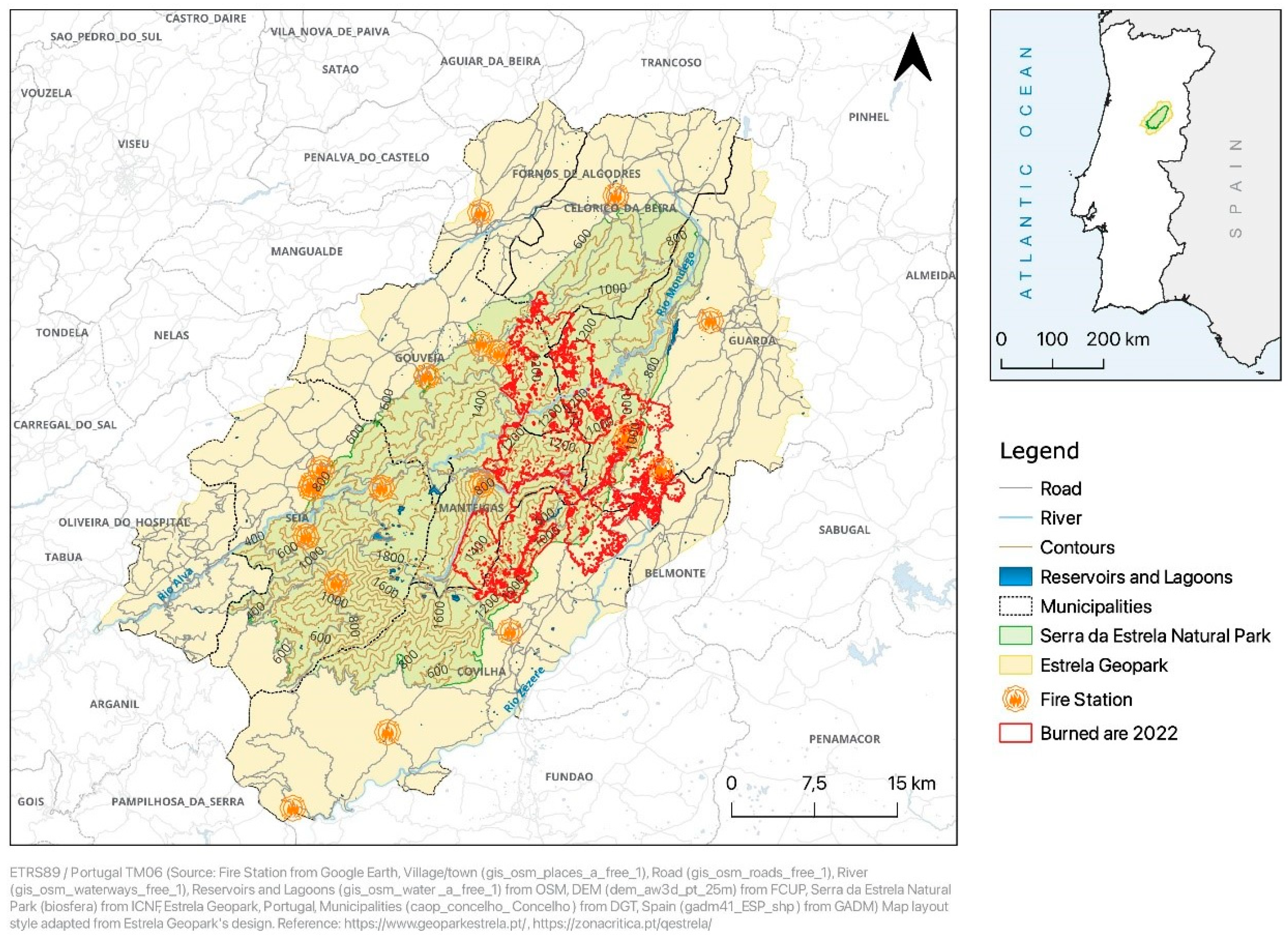
Figure 2.
Methodology diagram.
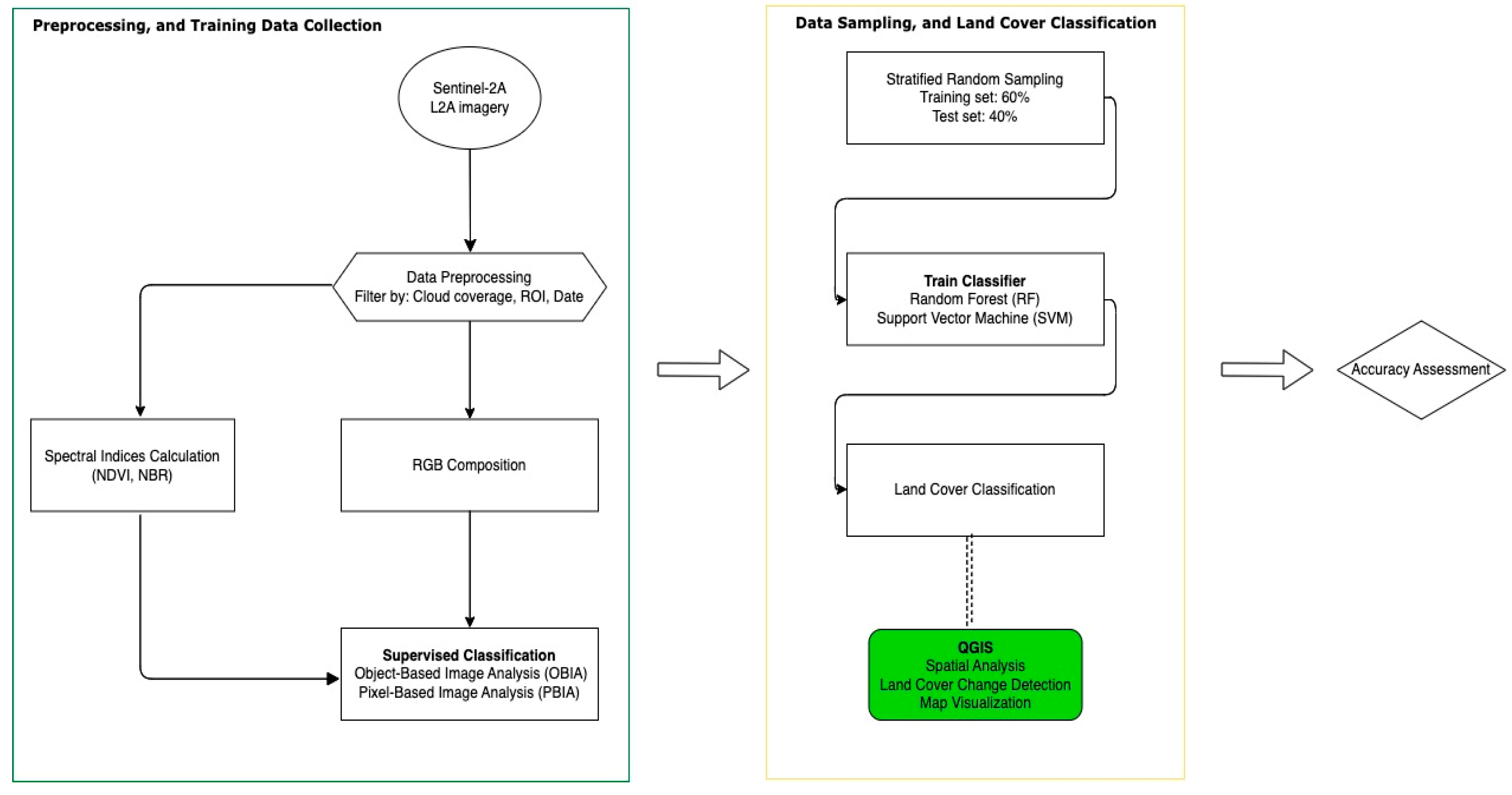
Figure 3.
The dNBR maps of the study area for the 2022 wildfire, based on classifications proposed by MLC (left), and UGSG (right).
Figure 3.
The dNBR maps of the study area for the 2022 wildfire, based on classifications proposed by MLC (left), and UGSG (right).
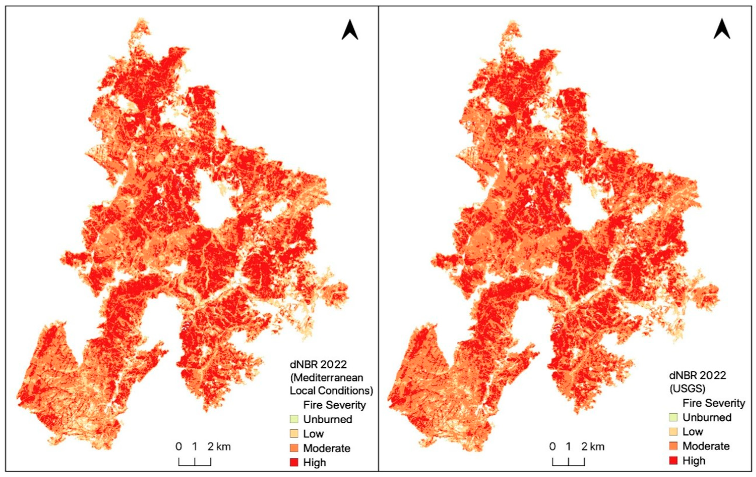
Figure 4.
NDVI maps of the study area for: (a) pre-wildfire 2022, (b) post-wildfire 2022, and (c) summer 2023, computation was made from Sentinel-2A data and classified according to NDVI values range suggested by USGS.
Figure 4.
NDVI maps of the study area for: (a) pre-wildfire 2022, (b) post-wildfire 2022, and (c) summer 2023, computation was made from Sentinel-2A data and classified according to NDVI values range suggested by USGS.
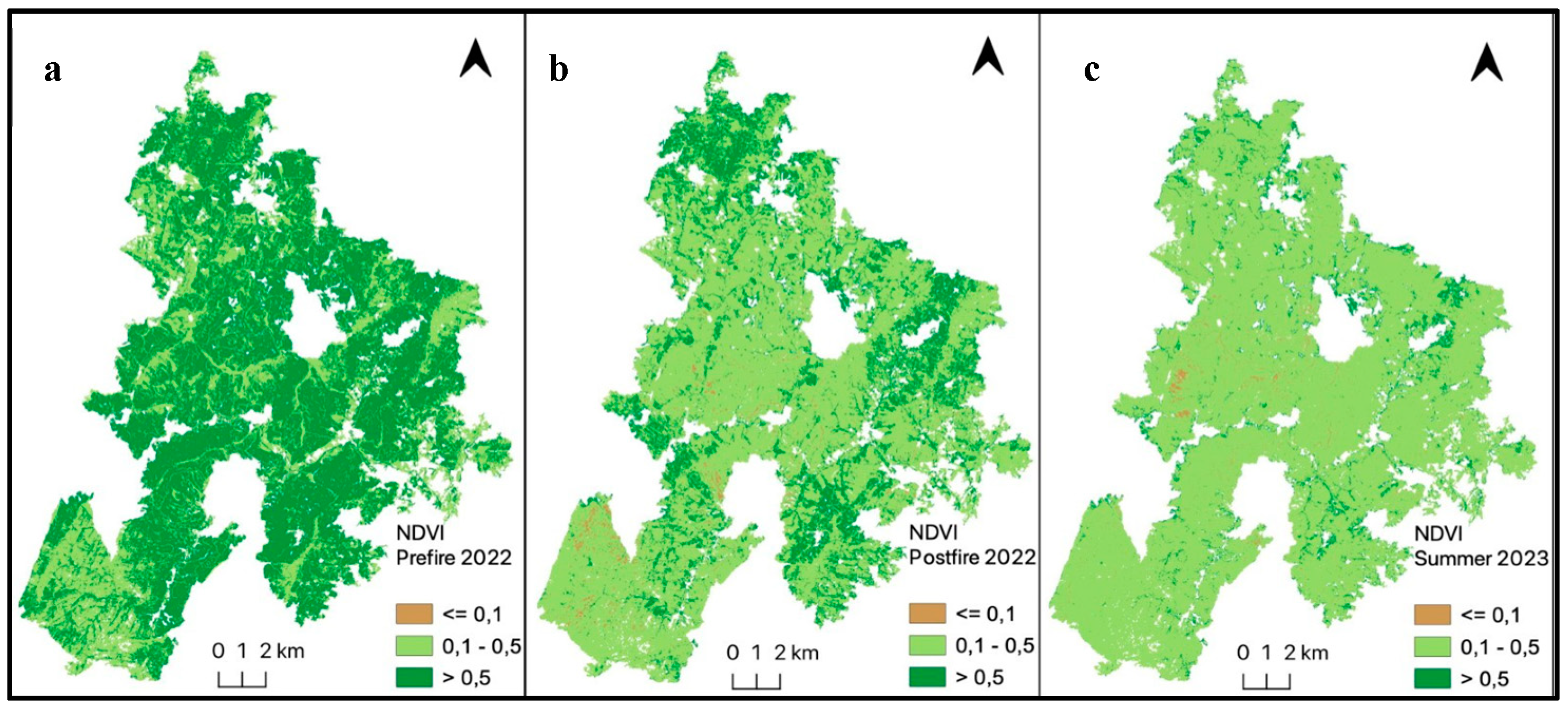
Figure 5.
F1 score ranking for different land cover classes across various models.
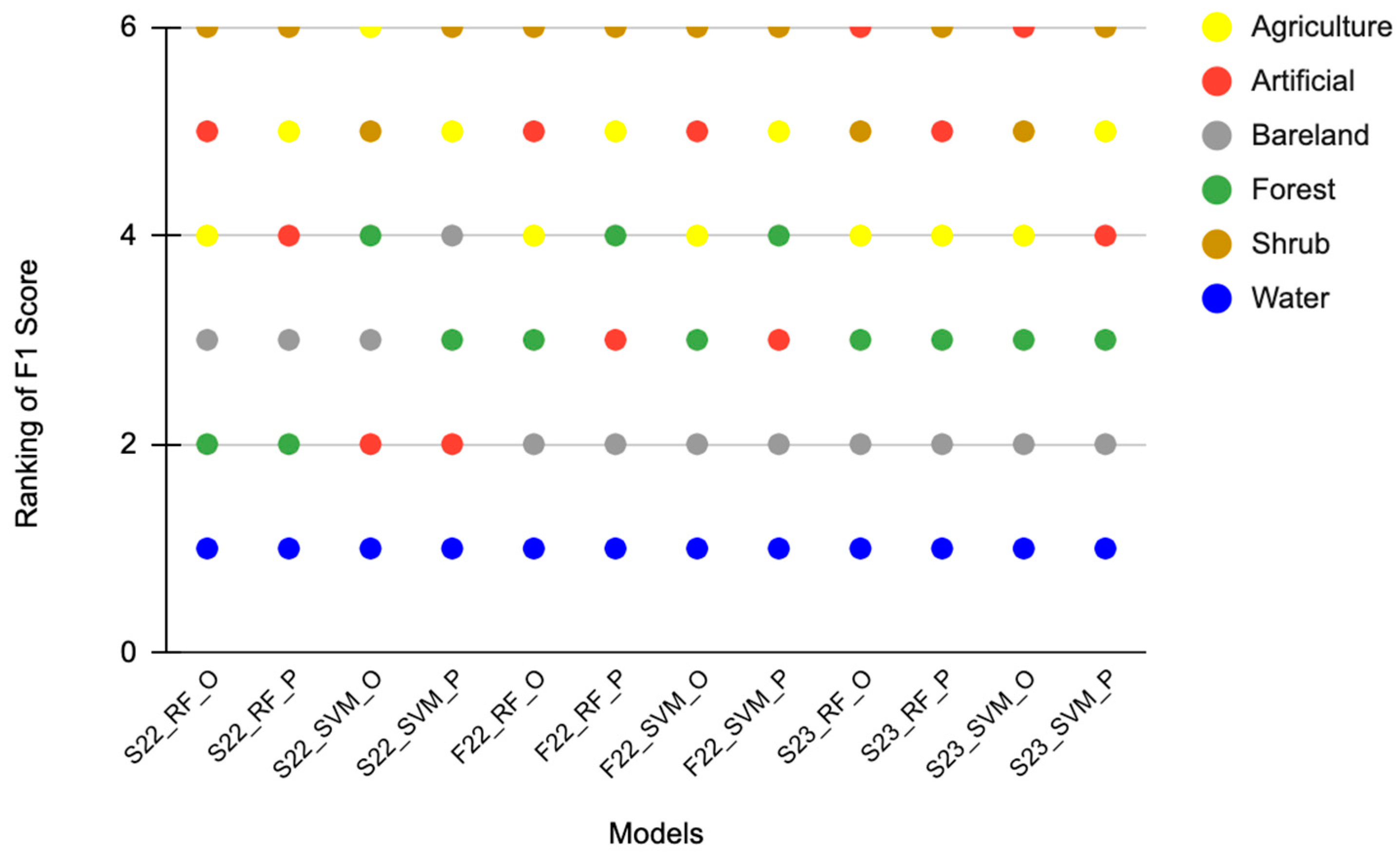
Figure 6.
Comparison of the burned area retrieved from ICNF (red border), and the post-wildfire land cover maps classified by different models: (a) RF x OBIA, (b) RF x PBIA, (c) SVM x OBIA, (d) SVM x PBIA.
Figure 6.
Comparison of the burned area retrieved from ICNF (red border), and the post-wildfire land cover maps classified by different models: (a) RF x OBIA, (b) RF x PBIA, (c) SVM x OBIA, (d) SVM x PBIA.
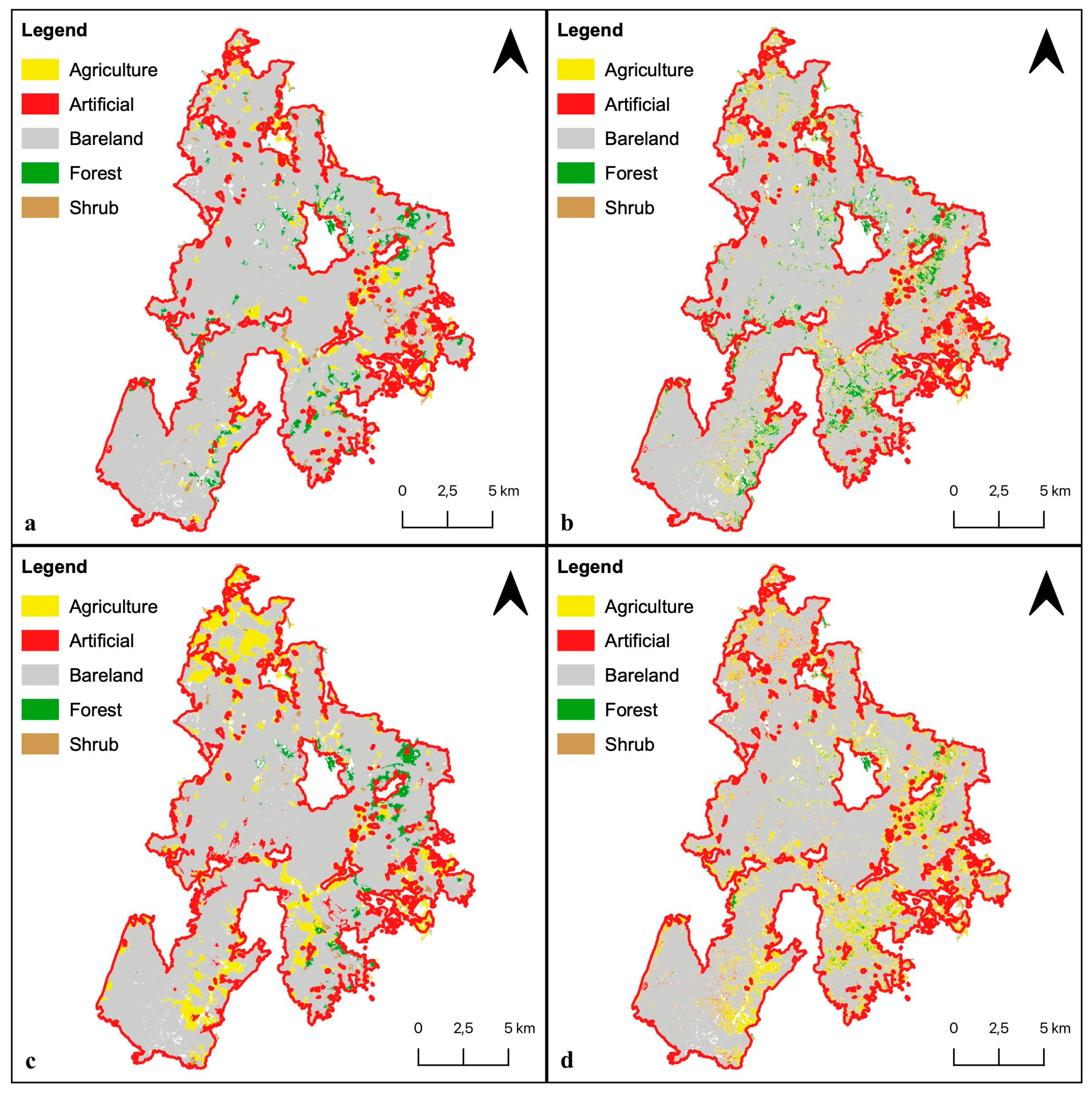
Figure 7.
Comparison of land cover maps classified by different models: (a) RF x OBIA, (b) RF x PBIA, (c) SVM x OBIA, (d) SVM x PBIA for pre-wildfire 2022.
Figure 7.
Comparison of land cover maps classified by different models: (a) RF x OBIA, (b) RF x PBIA, (c) SVM x OBIA, (d) SVM x PBIA for pre-wildfire 2022.
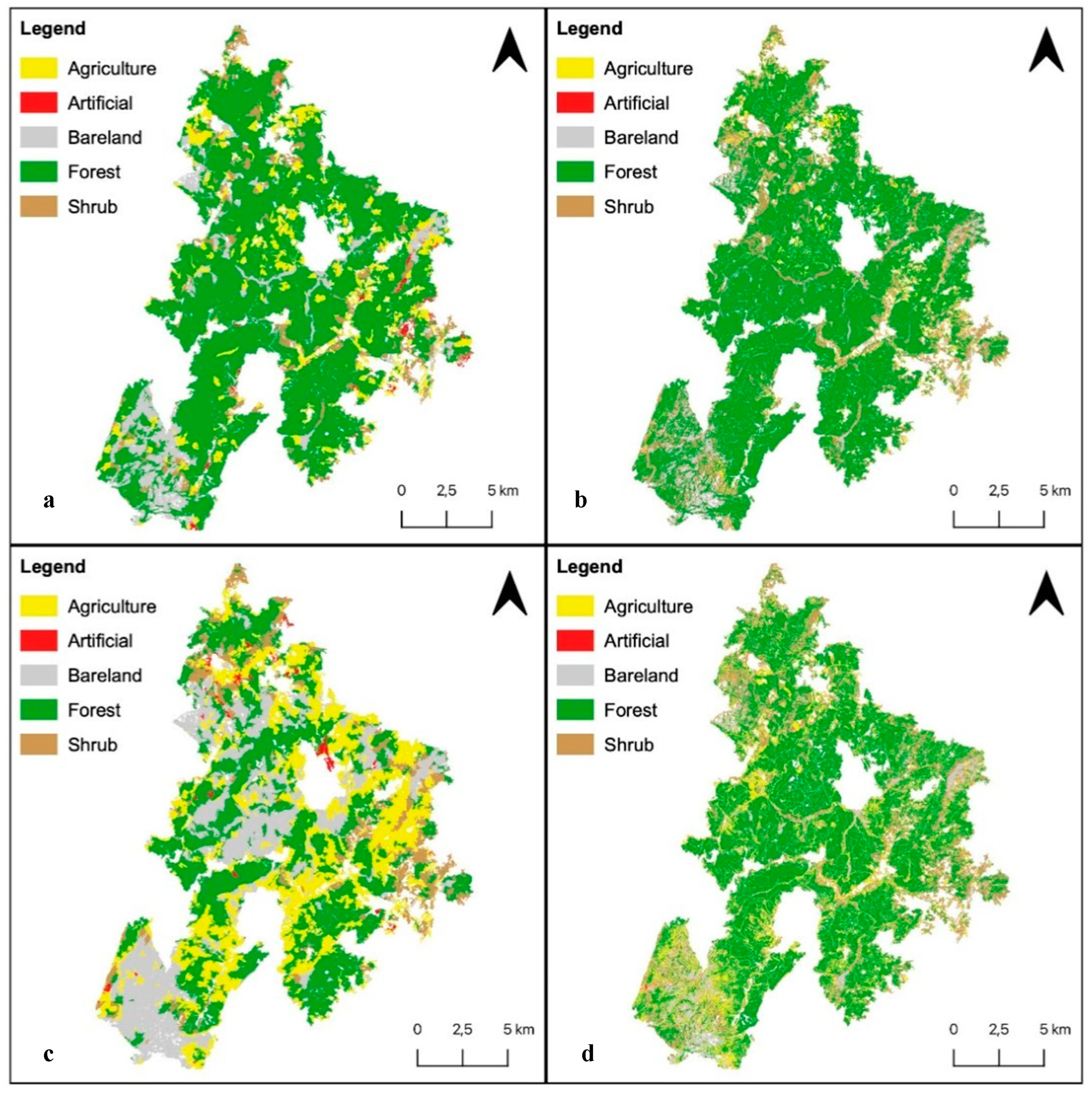
Figure 8.
COSc 2023.
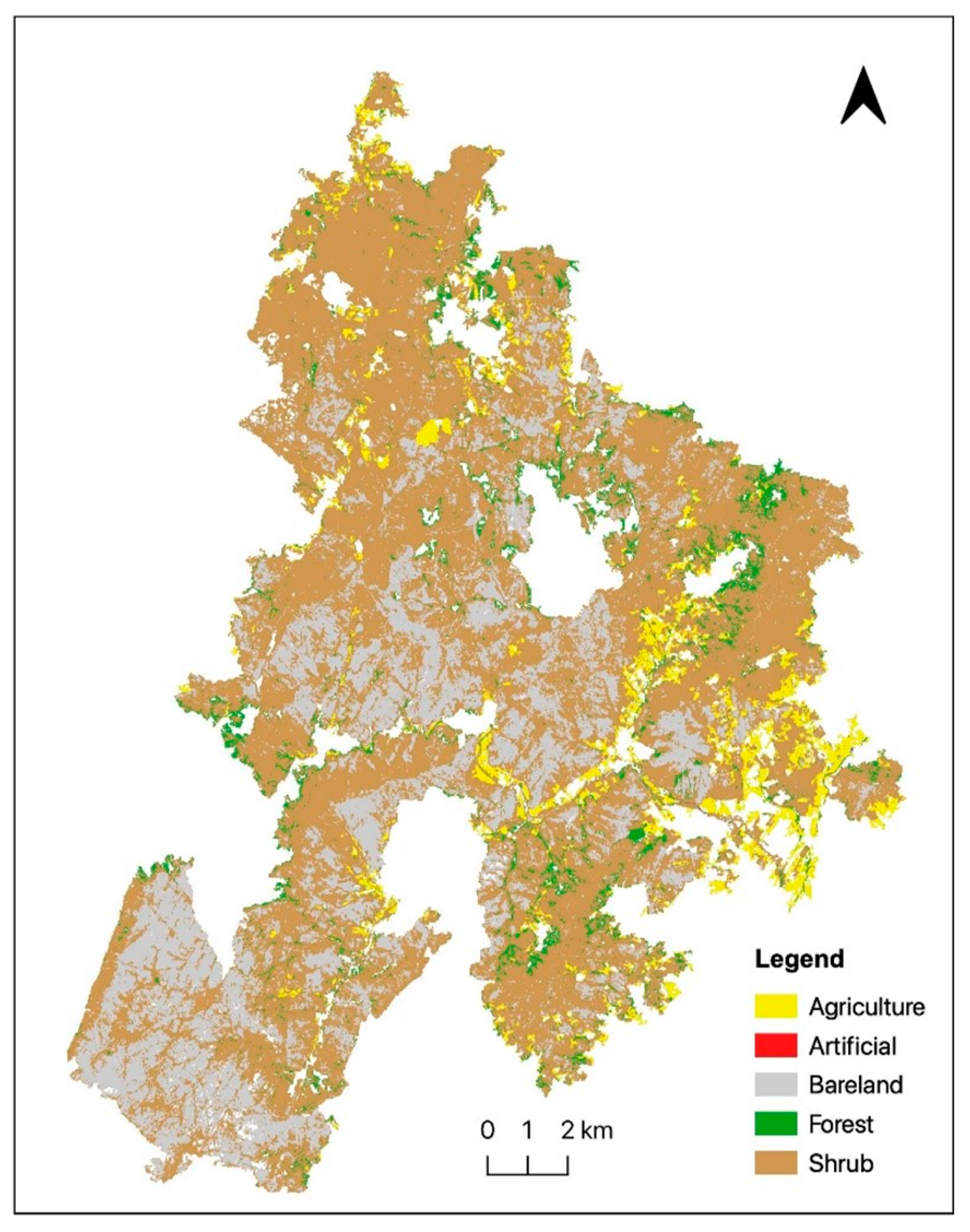
Figure 9.
Comparison of land cover maps classified by different models: (a) RF x OBIA, (b) RF x PBIA, (c) SVM x OBIA, (d) SVM x PBIA for summer 2023.
Figure 9.
Comparison of land cover maps classified by different models: (a) RF x OBIA, (b) RF x PBIA, (c) SVM x OBIA, (d) SVM x PBIA for summer 2023.
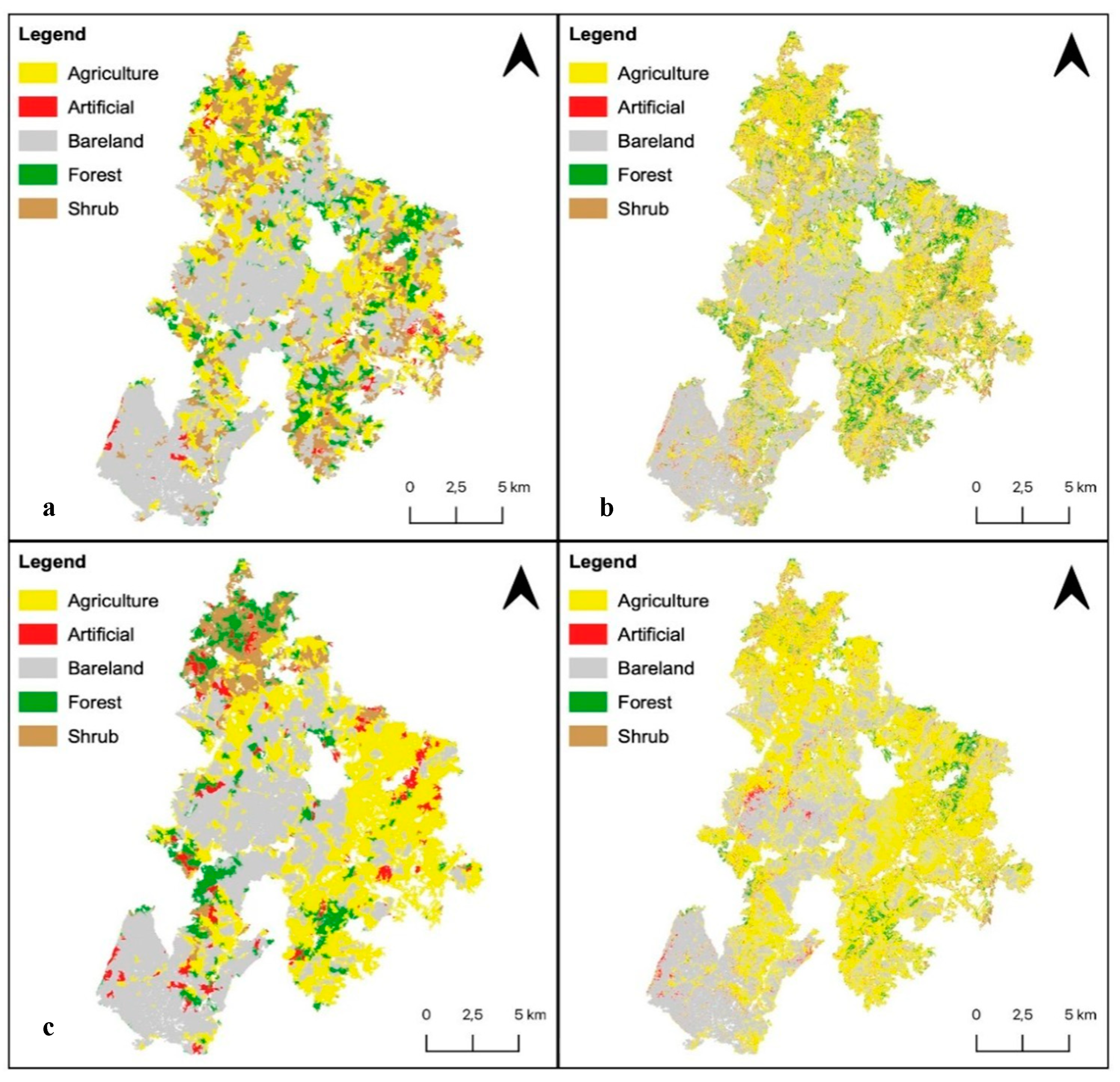
Figure 10.
The land cover maps classified using RF x OBIA model: (a) pre-wildfire 2022, (b) post-wildfire, and (c) summer 2023.
Figure 10.
The land cover maps classified using RF x OBIA model: (a) pre-wildfire 2022, (b) post-wildfire, and (c) summer 2023.
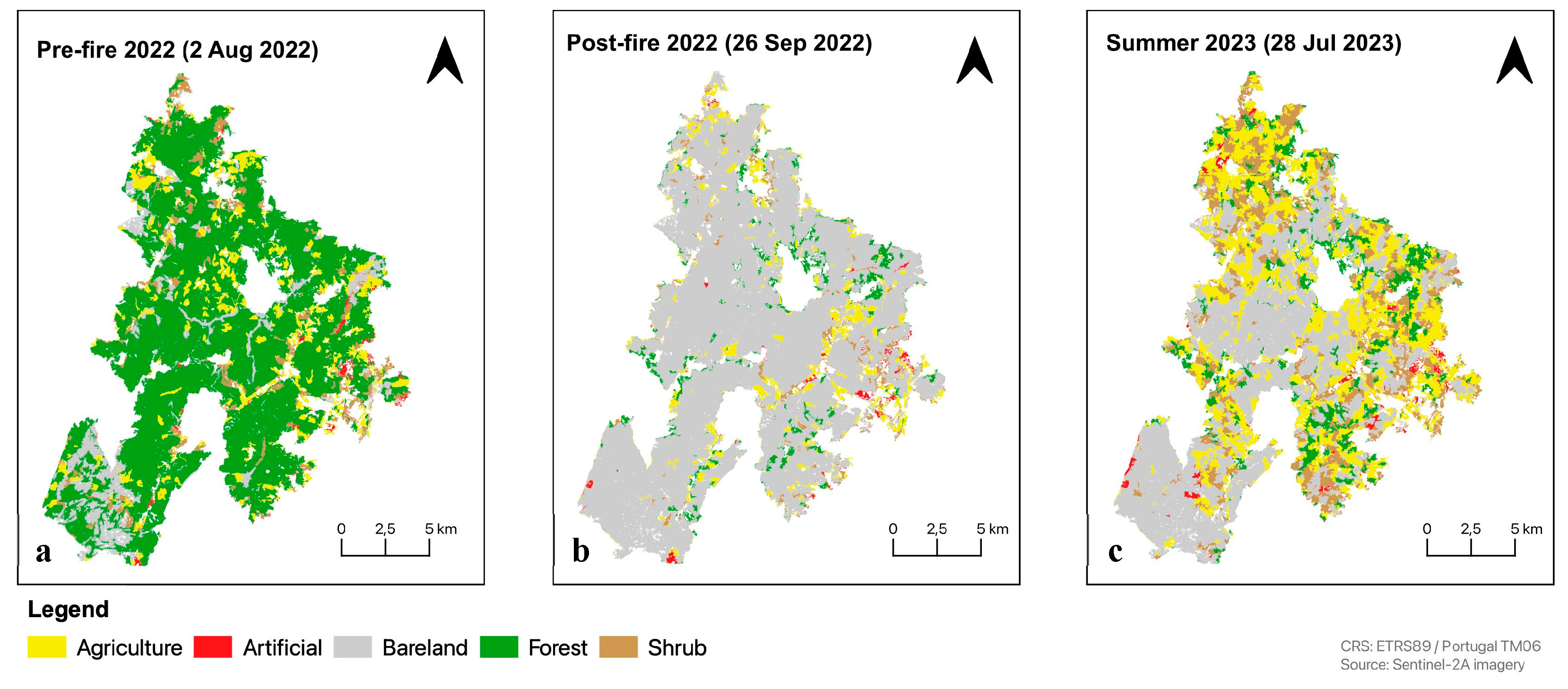
Figure 11.
The land cover maps classified using SVM x PBIA model: (a) pre-wildfire 2022, (b) post-wildfire, and (c) summer 2023.
Figure 11.
The land cover maps classified using SVM x PBIA model: (a) pre-wildfire 2022, (b) post-wildfire, and (c) summer 2023.
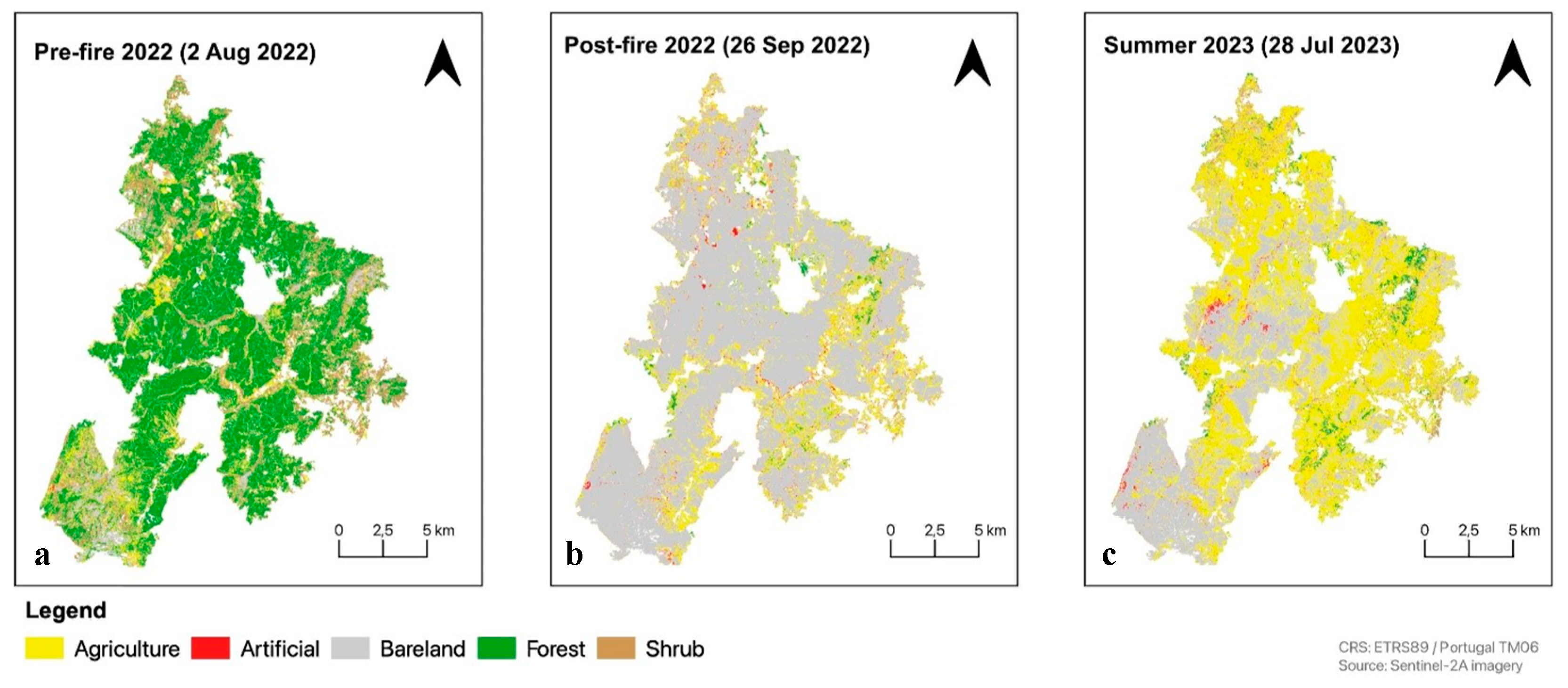

Table 1.
Sentinel-2A imageries applied in this study.
| Acquisition Date | Event | Cloud cover (%) |
|---|---|---|
| 2 August 2022 | Pre-wildfire 2022 | 0.000657 |
| 26 September 2022 | Post-wildfire 2022 | 0.152309 |
| 28 July 2023 | Summer 2023 (1 Year after fire) |
0.000352 |
Table 2.
Description of the 6 land cover classes used in this research.
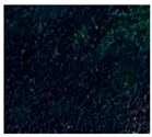
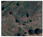
| ID | Class/Level 1 | Level 3 | Satellite image |
|---|---|---|---|
| 0 | 2 - Agriculture | 211- Autumn/winter annual crops 212 - Spring/summer annual crops 213 - Other agricultural areas |
 |
| 1 | 1 - Artificial | 100 - Artificial areas | 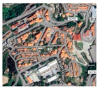 |
| 2 | 5 - Bareland |
500 - Surface without vegetation |
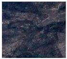 |
| 3 | 3 - Forest |
311 - Cork oak and holm oak 312 - Eucalyptus 313 - Other hardwoods 321 - Maritime pine 323 - Other resinous plants |
 |
| 4 | 4 - Shrub | 410 - Shrub 420 - Spontaneous herbaceous vegetation |
 |
| 5 | 6 - Water | 620 - Water |  |
Table 3.
Analysis of the land area affected by different fire severities in the study area after the 2022 wildfire, based on the dNBR ranges proposed by MLC and USGS.
Table 3.
Analysis of the land area affected by different fire severities in the study area after the 2022 wildfire, based on the dNBR ranges proposed by MLC and USGS.
| Fire Severity | dNBR range (scaled by 103) | MLC (100m2) |
% | dNBR range (scaled by 103) | USGS (100m2) |
% |
|---|---|---|---|---|---|---|
| Unburned | <= 100 | 53291 | 2.20 | <= 100 | 53291 | 2.20 |
| Low | 100 - 320 | 409450 | 16.89 | 100 - 270 | 292044 | 12.05 |
| Moderate | 320 - 650 | 1042929 | 43.03 | 270 - 660 | 1193272 | 49.23 |
| High | > 650 | 918192 | 37.88 | > 660 | 885255 | 36.52 |
| Total | 2423862 | 100 | 2423862 | 100 |
Table 4.
Analysis of the study area size subject to NDVI values range suggested by USGS.
| NDVI | Pre-wildfire 2022 (100m2) | % | Post-wildfire 2022 (100m2) | % | Summer 2023 (100m2) | % |
|---|---|---|---|---|---|---|
| <= 0.1 | 647 | 0.03 | 23563 | 0.98 | 25378 | 1.05 |
| 0.1 - 0.5 | 844708 | 34.85 | 2229573 | 91.98 | 1820739 | 75.11 |
| > 0.5 | 1578507 | 65.12 | 170726 | 7.04 | 577745 | 23.84 |
| Total | 2423862 | 100 | 2423862 | 100 | 2423862 | 100 |
Table 5.
Confusion Matrix of SVM x PBIA model [Post-wildfire 2022].
| SVM x PBIA | Agriculture | Artificial | Bareland | Forest | Shrub | Water | Precision |
|---|---|---|---|---|---|---|---|
| Agriculture | 797 | 2 | 16 | 249 | 79 | 0 | 0.6973 |
| Artificial | 11 | 207 | 6 | 0 | 0 | 0 | 0.9241 |
| Bareland | 18 | 13 | 2554 | 0 | 0 | 0 | 0.988 |
| Forest | 185 | 0 | 0 | 860 | 11 | 0 | 0.8144 |
| Shrub | 223 | 2 | 0 | 11 | 83 | 0 | 0.2602 |
| Water | 0 | 0 | 0 | 0 | 0 | 53 | 1 |
| Recall | 0.6459 | 0.9241 | 0.9915 | 0.7679 | 0.4798 | 1 |
Table 6.
Overall accuracy and kappa coefficient of each model.
| RF x OBIA | RF x PBIA | SVM x OBIA | SVM x PBIA | |||||
|---|---|---|---|---|---|---|---|---|
| OA | κ | OA | κ | OA | κ | OA | κ | |
| Pre-fire 2022 | 0.99 | 0.98 | 0.90 | 0.86 | 0.74 | 0.66 | 0.81 | 0.73 |
| Post-fire 2022 | 0.99 | 0.98 | 0.94 | 0.91 | 0.84 | 0.76 | 0.85 | 0.77 |
| Summer 2023 | 0.99 | 0.99 | 0.94 | 0.91 | 0.97 | 0.96 | 0.88 | 0.83 |
Table 7.
Analysis of the land cover size after wildfire 2022 for each model.
| F22 | RF x OBIA | RF x PBIA | SVM x OBIA | SVM x PBIA | ||||
|---|---|---|---|---|---|---|---|---|
| Class | Area (ha) | % | Area (ha) | % | Area (ha) | % | Area (ha) | % |
| 0 | 1,655.68 | 6.83 | 2,989.13 | 12.33 | 3,684.57 | 15.20 | 5,172.30 | 21.34 |
| 1 | 191.49 | 0.79 | 373.98 | 1.54 | 639.68 | 2.64 | 593.50 | 2.45 |
| 2 | 20,512.27 | 84.63 | 18,566.33 | 76.60 | 18,710.02 | 77.19 | 17,346.21 | 71.56 |
| 3 | 1,152.91 | 4.76 | 1,527.02 | 6.30 | 754.61 | 3.11 | 391,02 | 1.61 |
| 4 | 724.23 | 2.99 | 779.75 | 3.22 | 447.71 | 1.85 | 733.09 | 3.02 |
Table 8.
Analysis of the land cover size in summer 2023 for each model and COSc 2023.
| Area(ha) | Agriculture | Artificial | Bareland | Forest | Shrub |
|---|---|---|---|---|---|
| COSc 2023 | 1479.32 | 5.78 | 5820.55 | 1168.25 | 15757.47 |
| RF_OBIA_S23 | 6867.58 | 349.50 | 10425.99 | 2316.96 | 4276.57 |
| RF_PBIA_S23 | 10254.29 | 187.83 | 8555.31 | 1892.89 | 3342.48 |
| SVM_OBIA_S23 | 9822.13 | 1041.57 | 9404.46 | 2196.01 | 1771.86 |
| SVM_PBIA_S23 | 14189.20 | 472.56 | 7944.88 | 752.46 | 876.15 |
Table 9.
Each land cover class's major land cover change from pre-fire 2022 to post-fire 2022, and from post-fire 2022 to summer 2023 [RF x OBIA model].
Table 9.
Each land cover class's major land cover change from pre-fire 2022 to post-fire 2022, and from post-fire 2022 to summer 2023 [RF x OBIA model].
| Major change from | Prefire 2022 to Postfire 2022 | Postfire 2022 to Summer 2023 | ||||
| To | Area (ha) | % | To | Area (ha) | % | |
| Agriculture | Bareland | 1593.07 | 6.57 | Agriculture | 690.74 | 2.85 |
| Artificial | Bareland | 70.53 | 0.29 | Artificial | 58.79 | 0.24 |
| Bareland | Bareland | 2094.21 | 8.64 | Bareland | 9965.35 | 41.11 |
| Forest | Bareland | 15847.11 | 65.38 | Forest | 653.9 | 2.7 |
| Shrub | Bareland | 907.34 | 3.74 | Agriculture | 302.43 | 1.25 |
Table 10.
The major land cover change of each land cover class from pre-fire 2022 to post-fire 2022, and from post-fire 2022 to summer 2023 [SVM x PBIA model].
Table 10.
The major land cover change of each land cover class from pre-fire 2022 to post-fire 2022, and from post-fire 2022 to summer 2023 [SVM x PBIA model].
| Major change from | Prefire 2022 to Postfire 2022 | Postfire 2022 to Summer 2023 | ||||
| To | Area (ha) | % | To | Area (ha) | % | |
| Agriculture | Bareland | 3305.88 | 13.64 | Agriculture | 3881.37 | 16.01 |
| Artificial | Bareland | 28.07 | 0.12 | Agriculture | 370.35 | 1.53 |
| Bareland | Bareland | 877.69 | 3.62 | Agriculture | 9354.4 | 38.59 |
| Forest | Bareland | 11373.65 | 46.92 | Forest | 243.37 | 1 |
| Shrub | Bareland | 1760.7 | 7.26 | Agriculture | 450.55 | 1.9 |
Table 11.
Land Cover Changes: Prefire 2022, Postfire 2022, and Summer 2023 [RF x OBIA].
| ID | Land Cover | Prefire 2022 | Postfire 2022 | Summer 2023 | |||
| Area (ha) | % | Area (ha) | % | Area (ha) | % | ||
| 0 | Agriculture | 2452.94 | 10.12 | 1655.68 | 6.83 | 6867.58 | 28.34 |
| 1 | Artificial | 173.57 | 0.72 | 191.49 | 0.79 | 349.5 | 1.44 |
| 2 | Bareland | 2256.58 | 9.31 | 20512.27 | 84.63 | 10425.99 | 43.02 |
| 3 | Forest | 17846.92 | 73.64 | 1152.91 | 4.76 | 2316.96 | 9.56 |
| 4 | Shrub | 1506.59 | 6.22 | 724.23 | 2.99 | 4276.57 | 17.65 |
| Total | 24236.6 | 100 | 24236.6 | 100 | 24236.6 | 100 | |
Table 12.
Land Cover Changes: Prefire 2022, Postfire 2022, and Summer 2023 [SVM x PBIA].
| ID | Land Cover | Prefire 2022 | Postfire 2022 | Summer 2023 | |||
| Area (ha) | % | Area (ha) | % | Area (ha) | % | ||
| 0 | Agriculture | 5292.29 | 21.83 | 5,172.30 | 21.34 | 14189.20 | 58.55 |
| 1 | Artificial | 63.35 | 0.26 | 593.50 | 2.45 | 472.56 | 1.95 |
| 2 | Bareland | 984.99 | 4.06 | 17,346.21 | 71.56 | 7944.88 | 32.78 |
| 3 | Forest | 14884.9 | 61.41 | 391,02 | 1.61 | 752.46 | 3.1 |
| 4 | Shrub | 3010.71 | 12.42 | 733.09 | 3.02 | 876.15 | 3.62 |
| Total | 24236.24 | 100 | 24236.12 | 100 | 24235.25 | 100 | |
Disclaimer/Publisher’s Note: The statements, opinions and data contained in all publications are solely those of the individual author(s) and contributor(s) and not of MDPI and/or the editor(s). MDPI and/or the editor(s) disclaim responsibility for any injury to people or property resulting from any ideas, methods, instructions or products referred to in the content. |
© 2024 by the authors. Licensee MDPI, Basel, Switzerland. This article is an open access article distributed under the terms and conditions of the Creative Commons Attribution (CC BY) license (http://creativecommons.org/licenses/by/4.0/).
Copyright: This open access article is published under a Creative Commons CC BY 4.0 license, which permit the free download, distribution, and reuse, provided that the author and preprint are cited in any reuse.


