1. Introduction
Implementation of artificial Intelligence in manufacturing and process industries is becoming a mandatory requirement for sustainable and reliable failure free operation in shop floor. Therefore, real time fault diagnosis and precision health assessment system is a need for effective maintenance program in industrial sector [
1]. Rapid advancement in the digital technologies and AI techniques have invited more attention from research and development in industrial sectors and particularly in condition monitoring of machines and related Industrial processes [
2]. In this modern word, there are many technological digital revolution with a focus on cyber physical and biological systems such as Artificial Intelligence, Machine learning, Deep learning, Robotics, Internet on Things, Virtual Reality, etc., In machining based industries, Identification of reliable condition monitoring system would allow to give clear picture about the healthiness of a machine which is a mandatory requirement to go for adaptive or corrective actions [
3]. There is always a high demand for an accurate online machine condition or fault diagnosis system using modern technologies to reduce downtime and to improve effective utilization of machineries in the production system [
4]. A well-structured predictive maintenance system will reduce economic stresses and give necessary precautions to avoid a stoppage in production line [
5]. Normally, maintenance engineers used to follow three traditional maintenance strategies such as breakdown maintenance, planned maintenance and predictive maintenance [
6]. Among the three maintenance methods, predictive maintenance is commonly used in industries for intelligent diagnosis. The intelligent diagnosis procedure can be applied in offline or online [
7]. Compared to offline techniques, online condition monitoring will do a continuous fault detection using sensors and data acquisition. The predictive maintenance methods can be broadly categorized as model based predictive maintenance and data based predictive maintenance. Model based is using a mathematical model based on empirical data to indicate a fault. But data driven method is using intelligent models like fuzzy logic, machine learning, deep learning etc. In the recent days, the data driven models are in align with machine learning, deep learning and digital twins. Machine learning and deep learning are the powerful tools of artificial intelligence that push the boundaries of innovation. Machine learning uses algorithms and learns on its own but it needs human assistance to correct errors. Deep learning uses advanced computing which uses much more data than machine learning. In deep learning, there is little or no human intervention while doing advanced computing. In condition monitoring, machine learning used thousands of data points while deep learning-based condition monitoring uses millions of data points. Machine learning based fault diagnosis methods are using explicit programming, but deep learning algorithms solve problem based on the layers of neural networks. Deep learning is a machine learning algorithm that uses deep (more than one layer) neural networks to analyze data and provide output accordingly. Koutsoupakin. j et al., discussed machine learning based condition monitoring for gear transmission systems using data generated by optimal multibody dynamic models. Even though, the title indicates machine learning, authors end up in their research with CNN which will normally come under deep learning techniques [
8]. Zhang. L et al., discussed an imbalanced fault diagnosis method based on TFFO and CNN for rotating machinery in which authors claimed that deep learning-based fault diagnosis usually requires a rich supply of data [
9]. Deep learning represented by MLP, CNN and RNN are the typical data driven fault diagnosis methods that enables end to end fault diagnosis without prior knowledge. In this work, three deep learning algorithms have been applied and an effective analysis have been done to identify a best solution in fault diagnosis of rotating machinery using unbalancing dataset.
2. Literature Review
2.1. Review Related to AI Models
Numerous methods of machine condition monitoring are investigated by fault diagnosis researchers which includes both direct and indirect methods. The direct methods like visual inspection, machine vision and Infra-red methodology are used to monitor the machine or machine tools which will give less accuracy compared to indirect methods [
10]. Indirect methods include use of signals like force, vibrations, acoustic emission etc., in which the signal features have a relationship with fault condition / parameters [
11]. Rui Zhao et al., have done a survey in his paper related to deep learning and its application to machine health monitoring. He has reviewed 108 technical articles and concluded in this way “It is believed that deep learning will have a more and more prospective future impacting machine health monitoring, especially in the age of big machinery data”. So, this survey is clearly indicating that the deep learning can be used in a precise way to monitor tool wear and also the paper concluded that the deep learning is a promising technique to assess tool wear [
12]. Lang Dai developed an Improved Deep Learning Model for Online Tool Condition Monitoring Using Output Power Signals. The output power from sensor which is mounted on cutting tool holder during its operation is used for analysis. This data is analyzed using wider first-layer kernels (WCONV), and long short-term memory (LSTM) which is available in deep learning algorithm. The weakness of the paper is addressing of output power signal. This paper is more focusing on the output power signals its analysis on deep learning algorithms which needs more study on the condition monitoring of the tool [
13]. Qun wang et al.,have done an overview of Tool Wear Monitoring Methods Based on Convolutional Neural Network. The authors concluded that it is feasible and reliable to apply convolution neural networks in tool wear and condition monitoring. They have added that the convolution neural network can improve the prediction accuracy, which is the great significance of the CNN technology [
14]. Convolutional neural networks (CNN) which is coming under deep learning, is a typical data-driven fault diagnosis method that extract features from images using convolutional layers, followed by pooling and fully connected layers for tasks like image classification [
15]. In condition monitoring, researchers have applied CNNs in fault diagnosis of rotating machinery. For instance, Janssens et al., proposed a feature learning model for condition monitoring based on CNN [
16]. Yao et al., used sound signal which is predicted using acoustic emission sensor and used CNN based on a multiscale dialog learning structure and attention mechanisms for gear fault prediction [
17]. Zhang, W et al., applied DCNN (Deep Convolutional neural networks) for bearing fault diagnosis under different operating loads [
18]. Abdelmaksoud M et al., proposed a (CNN) model to diagnose induction motor faults in the starting time of the motor. The model used to detect various faults locked-rotor, overload, voltage-unbalance, overvoltage, and undervoltage under three loading levels of Light, Normal, and Heavy loads. The authors concluded that deep CNN is an effective tool for diagnosing multi-signals induction motor faults at its starting period with different versions of datasets [
19].
2.2. Review Related to MLP
Marwala, T used multi-layer perceptron (MLP) for condition monitoring in a mechanical system. In this paper MLP is used to identify false in a population of cylindrical shells [
20]. Zanic, D. and Zuban, A. discussed the monitoring of transformer using MLP machine learning model. This paper describes the multi-layer perceptron class of artificial intelligence to predict temperature in transformer by giving three input features in MLP (oil temperature, winding current and outside temperature) [
21]. So, it is clear that the conventional MLP has been applied in the field of machine health condition monitoring for many years [
12].
Nguyen,V.Q et al., applied MLP mixer model for bearing fault diagnosis. The authors concluded that the Evaluation results show that the proposed MLP mixer model obtains high accuracy when the number of training samples are reduced. The authors added that the performance of the proposed model when compared with another state of arts proved the advantages of the MLP approach [
22]. Tarek, K et al., proposed an Optimized multi-layer perceptron for fault diagnosis of induction motor using vibration signals. The authors concluded that the obtained results show the capability of detecting faults in the induction motor under different operating conditions [
23].
2.3. Review Related to CNN
Neupane, D et al.,discussed coevolutionary neural network-based fault deduction for smart manufacturing. The result of this paper shows 1-D CNN is more efficient in terms of computational complex for time series data [
24]. With advancements in AI, researchers without any expertise can solve fault identification problems with bearings and gearbox [
25]. To extract the failure features from the signals, artificial neural networks, support vector machines, particle filter [
26], and extreme learning machines [
27] were used. In recent times, deep learning algorithms have been applied in rotating machine fault diagnosis due to their nonlinear regression ability [
27]. Some of these are Convolution Neural Network [
28,
29], Recurrent Neural Network [
30], Deep encoder, and Generative Adversarial Networks [
31]. Nonlinearities are common in real-world time series data [
32] , which makes it difficult to apply conventional prediction techniques [
33]. To address this issue, advanced techniques such as CNN, LSTM, and quantile regression were applied to predict failures. One-dimensional convolutional neural network is utilized for time series prediction [
34]. Zhang et al. stated that higher accuracy is achieved using DNN for time sequence prediction [
35]. Ruan, D et al., used CNN for bearing fault detection by giving fault period under different fault types and shaft rotation frequency were used to determine the size of CNN’s input. In the paper, authors confirmed that physics -guided CNN (PGCNN) with rectangular convolution kernel works better than the baseline CNN with more accuracy and less certainty [
36]. Kothuru,A et al.,applied deep visualization technique to gain knowledge on inner workings of the deep learning models in tool wear prediction for end milling. The authors concluded that CNN model focuses more on frequency features of the signal compared to the features with respect to time period of signal [
37]. However, CNN suffer from the weaknesses of not considering the imbalanced distribution of machinery health conditions and What CNNs have learned in predicting fault diagnosis is not clear. Jia, F et al., suggested a framework called deep normalized convolutional neural network (DNCNN) for imbalanced fault classification of machinery to overcome the first weakness. He has proposed neuron activation maximization (NAM) algorithm to handle the weakness of What CNNs have learned in predicting fault diagnosis [
38].
2.4. Review Related to RNN and LSTM
Elman’s recurrent neural network (RNN) is used by serhat seker et al., for condition monitoring in nuclear power plant and rotating machining. The first part of this work is prediction of anomalies in gas cooled nuclear reactor. The second part is the detection of motor bearing damage in induction motors [
39]. Halliday, C et al., applied RNN for condition monitoring and predictive maintenance of pressure vessel components. The authors found RNN is well suiting to tackle the shortfalls in RNN-ROM (Residual Order Models) [
40]. Swetha R Kumar and Jayaprasanth Devakumar used RNN with 10 hidden neurons to estimate state variables with the inputs and outputs of the process.The authors studied the effectiveness of RNN in fault detection and isolation for different scenarios of sensor’s output such as drift, erratic, hard-over, spike and stuck[
41]. Yahui Zhang et al., proposed a Gated Recurrent Unit (GRU) and MLP based model for fault diagnosis to detect fault types. In this work, One-dimensional time-series vibration signals converted into two-dimensional images in the first phase. Then, (GRU) is introduced to exploit sequential information of time-series data and learn representative features from constructed images. Then, An MLP is used to implement fault recognition. The results show that the proposed method gives the best result on two public datasets compared with existing work and shows the robustness against the noise [
42].
Zhuang Ye and Jianbo Yu applied long short-term memory (LSTM) unit to capture sequential information from multi sensor time series data. The authors used convolution calculation for noise reduction and feature extraction. In the end Health Index (HI) is generated based on reconstruction error of run-to-fail data [
43]. Zhao,H, Sun,S and Jin,B applied LSTM neural network based fault diagnosis. The authors indicated that LSTM can directly classify the raw process data without specific feature extraction and classifier design. In this work, LSTM to fault identification and analysis is evaluated in the Tennessee Eastman benchmark process. The authors used LSTM to capture sequential information from multi sensor time series data. In this work convolution calculation is utilized for noise reduction and feature extraction multivariate gaussian distribution is used to generate health index based of reconstruction errors of long short-term memory convolutional auto encoder [
44]. Afridi, Y.S et al., have developed a fault prognostic system using long short-term memory for rolling element bearing because of a greater number of critical elements bearing because of critical component involved and highest fault diagnosis [
45].
So, Deep learning architectures include deep belief network (DBN), Multilayer Perceptron (MLP), autoencoder (AE), convolutional neural network (CNN), and RNN [
46]. With the rapid development of DL techniques in these years, many new architectures have been proposed and introduced into the tasks of intelligent industrial fault diagnosis. Similarly, CNN is prospering again, due to the progress made in the fields of computer vision and enhanced visualization techniques in recent years [
47].
3. Spectra Quest Machinery Fault Simulator (SQMFS) – An Overview
In this research work, the Spectra Quest Machinery Fault Simulator (SQMFS) is utilized to simulate both balanced and imbalanced conditions of a rotary shaft. The Machine Fault Simulator (MFS) is a highly versatile and modular test platform designed to facilitate the study and simulation of various mechanical faults in rotating machinery. It is extensively used in academia, industry training, and research to provide a controlled environment for replicating real-world fault conditions, enabling comprehensive analysis and predictive maintenance. The simulator allows for the monitoring and analysis of fault conditions, providing valuable insights into vibration analysis and fault diagnostics [
48].
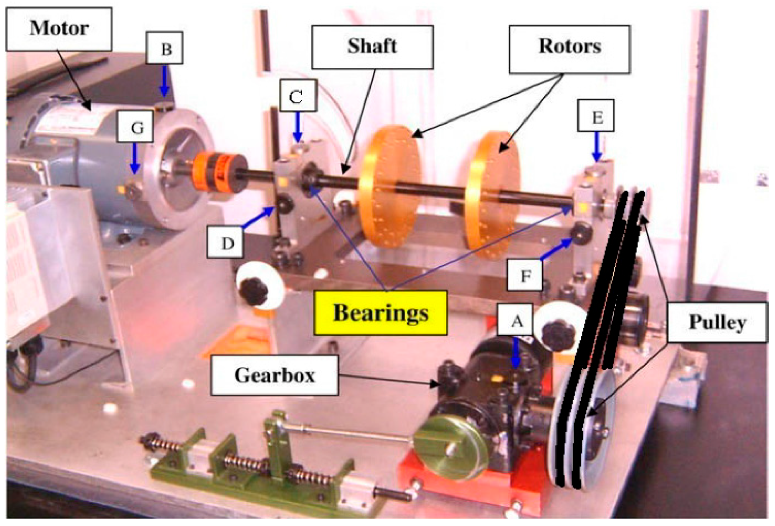
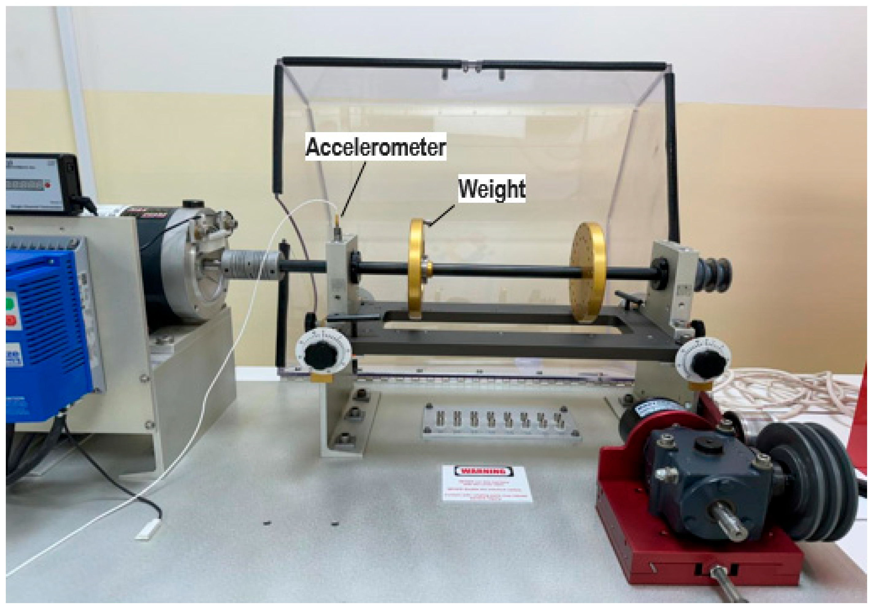
Figure 1 shows the photograph of SQMFS with the critical components involved in SQMFS.
The heart of the MFS is the motor-driven shaft, which serves as the primary rotating element where faults can be introduced and studied. The motor allows for variable speed control, which is crucial for observing the mechanical behavior of the system under different operating conditions. Precise speed adjustments enable the examination of how faults manifest across various frequencies and loads, thereby providing a comprehensive understanding of the system’s dynamics.
The MFS includes multiple adjustable disks and couplings that are mounted onto the shaft. These components are specifically designed with multiple tapped holes to accommodate the attachment of screws, weights, and other accessories. This flexibility is vital for simulating different fault conditions, such as unbalance, misalignment, or looseness. For instance, introducing an imbalance involves asymmetrically adding weights to the disks, which leads to uneven mass distribution and the characteristic vibration patterns of unbalanced systems. Strategically placed tapped holes on the disks allow for the precise positioning of weights, enabling the controlled introduction of imbalances. By varying the size and placement of these weights, researchers can replicate a wide range of imbalance severities, from mild to extreme, providing insights into the effects of different levels of imbalance on machine behavior. These couplings connect various rotating components and can be adjusted to introduce misalignments, which are common faults in rotating machinery. This feature is essential for simulating both angular and parallel misalignments, which can cause significant changes in vibration patterns and lead to mechanical failure if left undetected. The shaft is supported by high-precision bearings that ensure smooth rotation while also allowing for the introduction of bearing faults. The MFS’s support structure is designed to be sturdy and minimizes external vibrations that could interfere with the data, ensuring that observed faults are due solely to the simulated conditions.
The MFS is equipped with various sensors, such as accelerometers, proximity probes, and load cells, to monitor vibrations, forces, and rotational speeds. These sensors are strategically placed to capture the data required for fault analysis. The placement of these sensors is configurable, allowing for targeted measurements aligned with the specific fault being studied.
The setup incorporates several critical components, including a motor-driven shaft, adjustable disks, a Lenze controller, and a data acquisition system, to facilitate accurate data collection and analysis. Before each test, the system is configured to simulate the specific fault condition under study. For example, to examine imbalance, weights are attached to the rotor disks at predetermined locations. The motor speed, managed by the Lenze Controller, is set to the desired level, ranging from low speeds (to observe subtle faults) to high speeds (to assess fault severity under real-world conditions).
As the shaft rotates, the introduced faults generate vibrations captured by the attached accelerometer. In imbalance studies, uneven mass distribution causes centrifugal forces that result in periodic vibrations, manifesting as distinct frequency spikes in the spectrum analysis. The sensors provide real-time data on these vibrations, allowing researchers to identify fault characteristics.
The MFS is integrated with a Lenze Controller, which provides precise control over motor speeds and torque during the simulation. This controller enables real-time adjustments of motor parameters such as speed, acceleration, and torque limits, essential for accurately replicating various fault conditions. The fine control provided by the Lenze Controller enhances the reliability and repeatability of fault simulations.
4. Experimental Setup of Unbalancing in Machine Fault Simulator
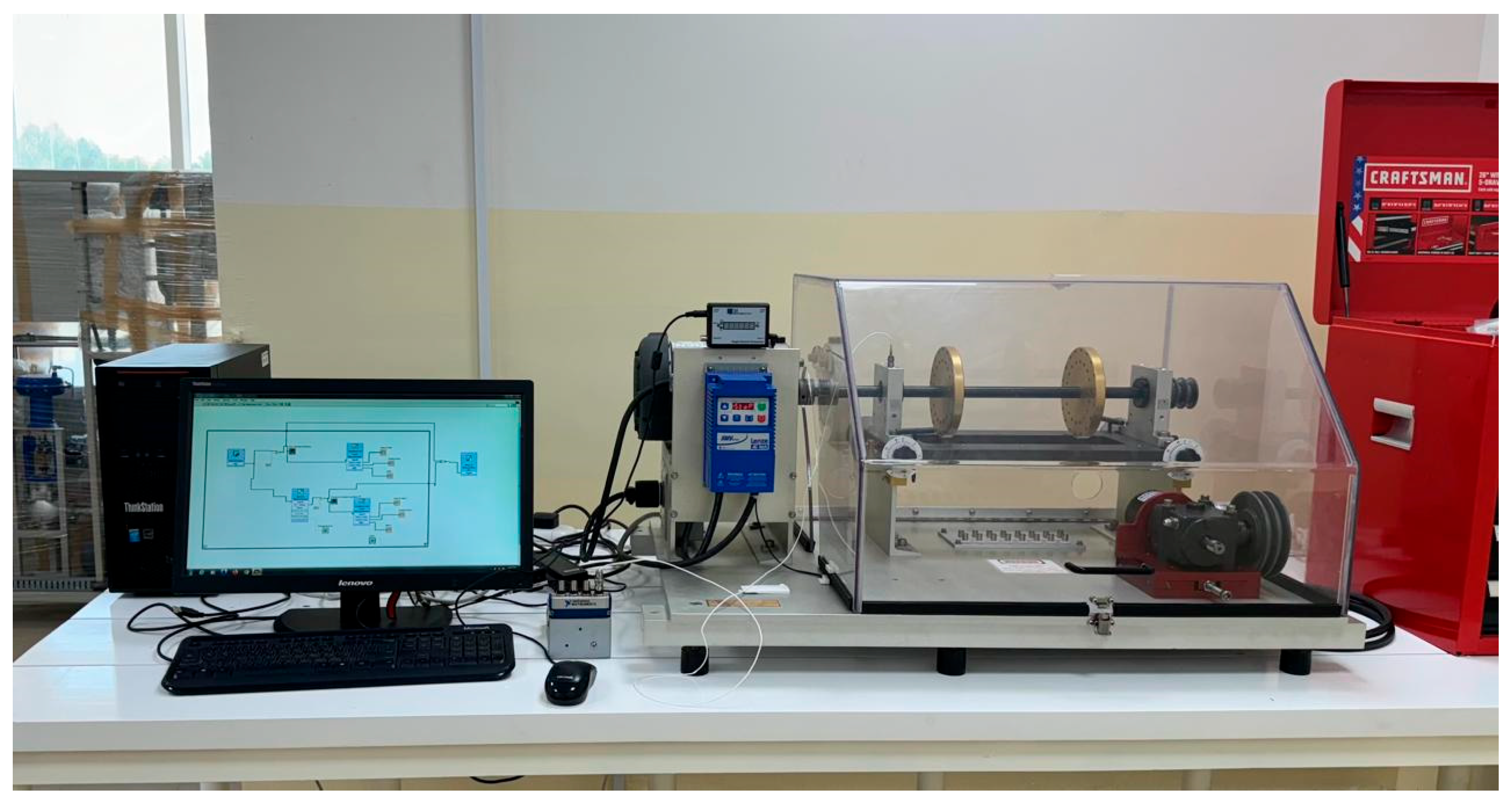
Figure 2 and
Figure 3 show the complete experimental setup of the Machinery Fault Simulator. On the left in
Figure 2, we can see a computer monitor displaying the LabVIEW interface used for data acquisition and analysis. In the center, there’s a blue Lenze Controller responsible for precise motor speed control. On the right, we see the MFS itself, enclosed in a transparent safety case. This setup allows for safe operation while providing clear visibility of the rotating components during experiments.
This close-up image of the MFS rotor provides a detailed view of the key components. We can see the motor-driven shaft, adjustable disks with tapped holes for attaching weights, and the accelerometer mounted to capture vibration data. The golden disk on the shaft is one of the adjustable disks used for introducing imbalance (
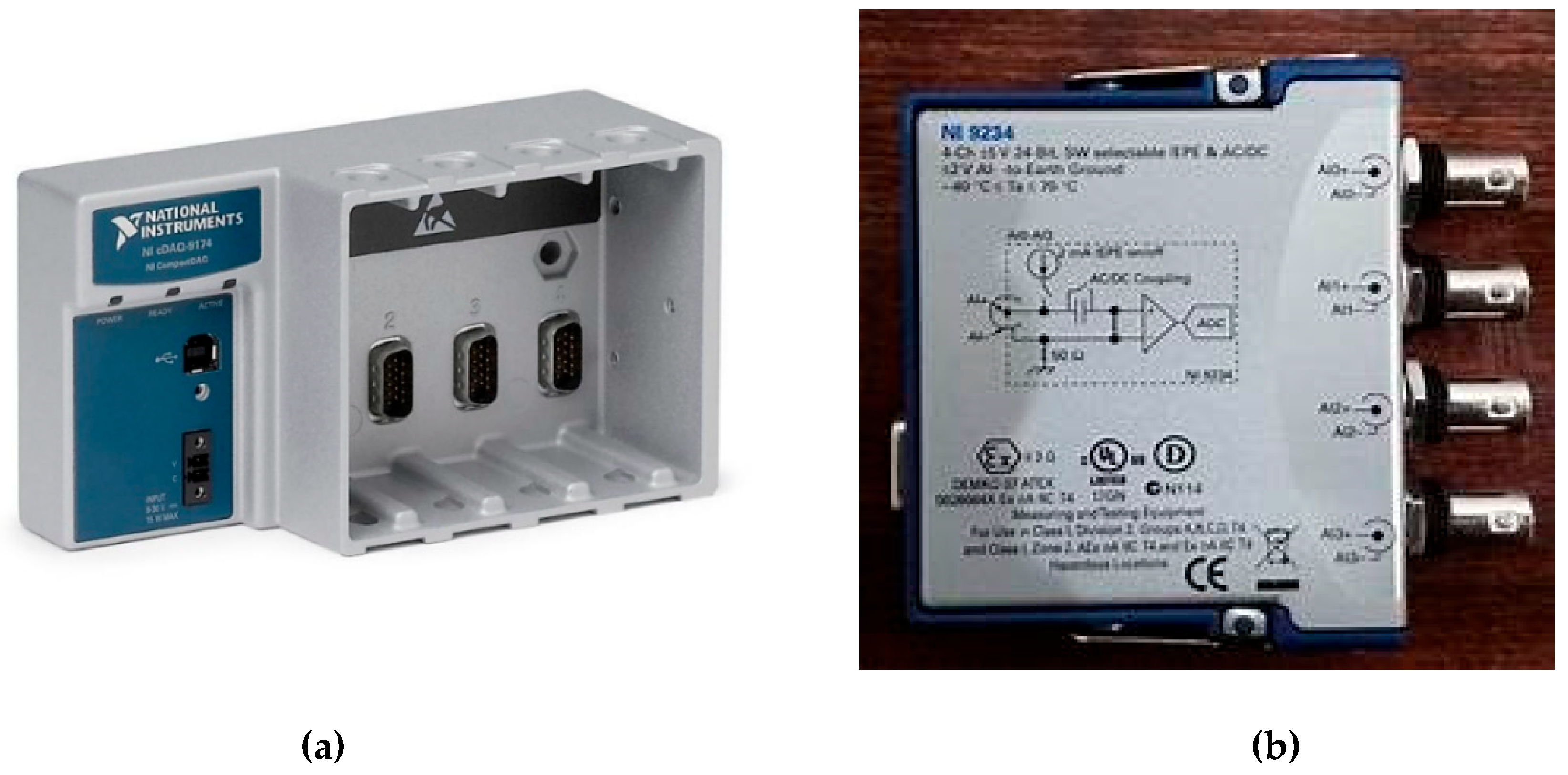
Figure 3). This configuration allows for precise control over the introduction of faults and the measurement of resulting vibrations. The data acquisition system, consisting of components like the National Instruments (NI) cDAQ-9174 (
Figure 4(a)) chassis and NI modules, captures vibration, displacement, and speed data from the sensors. The NI cDAQ-9174 is a modular chassis that serves as the central data acquisition hub, with slots for various C Series I/O modules, such as the NI 9234 (
Figure 4(b)) Dynamic Signal Acquisition Module for high-precision dynamic signal acquisition. The accelerometer, strategically mounted on the rotary shaft, measures both radial and axial vibration data. The collected data is transmitted to specialized software like LabVIEW for visualization, allowing researchers to interpret and diagnose fault conditions accurately. The NI 9234 module, inserted into one of the slots of the cDAQ-9174 chassis, is specifically designed for high-precision dynamic signal acquisition. It features four analog input channels with built-in anti-aliasing filters, capable of sampling up to 51.2 kS/s per channel. This module is essential for capturing subtle variations in vibration patterns and detecting early signs of mechanical faults. It supports a wide range of sensor types, including accelerometers, making it suitable for vibration analysis in rotating machinery.
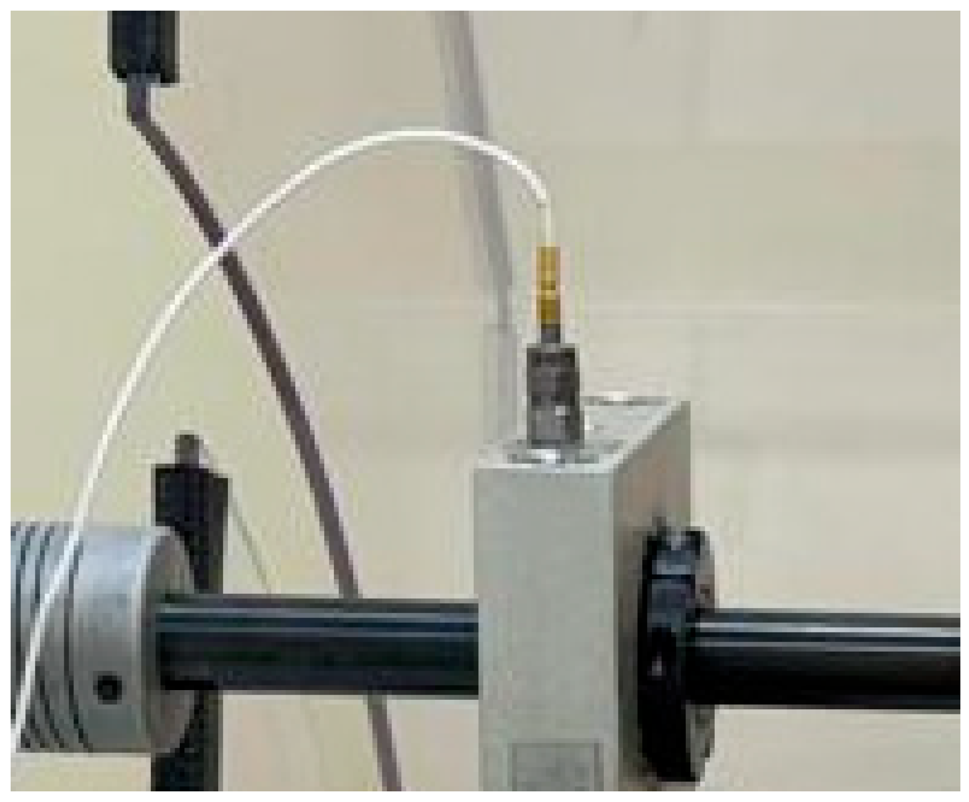
The accelerometer (mounted vertically on the rotary shaft in
Figure 5) is a critical sensor for measuring vibrations resulting from shaft rotation. It captures both radial and axial vibration data, providing insights into the dynamic behavior of the shaft under balanced and imbalanced conditions. The vertical placement of the accelerometer is strategic, as it enhances sensitivity to vibrations caused by imbalances, thereby improving fault detection accuracy.
This integrated experimental setup enables in-depth analysis and understanding of machine behavior under simulated fault conditions, enhancing the reliability of fault detection methods and contributing to the development of more robust machinery monitoring systems.
5. Data Collection and Signal Preprocessing
The experimental analysis focused on two primary operating conditions of the rotary shaft:
Balanced Condition
Imbalanced Condition
These conditions were carefully established to study the effects of imbalance on the dynamic behavior of rotating machinery, thereby providing critical insights for developing diagnostic tools.
5.1. Balancing condition in MFS
Balancing plays a crucial role in operating the MFS, particularly when examining the effects of imbalance on machinery health. Balancing ensures uniform mass distribution in rotating components, thereby minimizing vibration, reducing bearing wear, and enhancing overall machinery performance. The MFS facilitates the study of these effects by allowing users to adjust the balance state of the shafts and observe the resulting changes in machine behavior.
The MFS uses an accelerometer to capture frequency and time-domain data, providing real-time insights into the impact of imbalance conditions. Weights are added or removed to the shaft disks to simulate unbalanced scenarios, replicating real-world conditions such as unbalanced rotors. This setup enables the detailed study of vibration patterns and highlights the significance of balancing in rotating machinery.
In the Balanced Condition, the rotary shaft was operated without any additional weights or defects. This state represented a perfectly balanced system, where the shaft’s mass was uniformly distributed across its entire length. By operating the machinery under this condition, baseline vibration data was collected. This baseline data served as a critical reference point for all subsequent analyses, providing a standard against which the effects of various imbalances could be measured.
Key aspects of the balanced condition include:
No Added Weights or Defects: Ensuring that no external weights, screws, or other defects were present on the rotary shaft, resulting in minimal vibration levels.
Uniform Mass Distribution: The rotary shaft’s weight was evenly distributed along its axis, resulting in smooth operation with low amplitude vibrations.
Data Collection as Baseline: Vibration data collected under these conditions provided a control sample, essential for differentiating between normal operational vibrations and those caused by faults or imbalances.
The balanced condition monitoring is very important in fault diagnosis to have comparison with unbalanced condition dataset.
5.2. Unbalancing condition in MFS
To simulate real-world conditions, an Imbalanced Condition was introduced by adding screws and weights of varying magnitudes to the rotary shaft disks on both the left and right sections. The controlled introduction of these weights was designed to replicate common mechanical faults, such as unbalance, that are often encountered in rotating machinery.
Key aspects of the imbalanced condition include:
Addition of Weights: Controlled weights, ranging from light screws to heavier attachments, were mounted on one side of the rotary shaft disks to create an intentional imbalance. This allowed for the simulation of different fault magnitudes, from minor to severe. The image below shows the weights attached to the rotary shaft.
Variable Weight Magnitudes: By varying the magnitude and distribution of the weights, different levels of imbalance were achieved, enabling the study of their effects on vibration patterns and machine behavior.
For the experiment the weights of each screw were taken for the imbalance before adding it to the shaft. The image below shows the device used to take the weights.
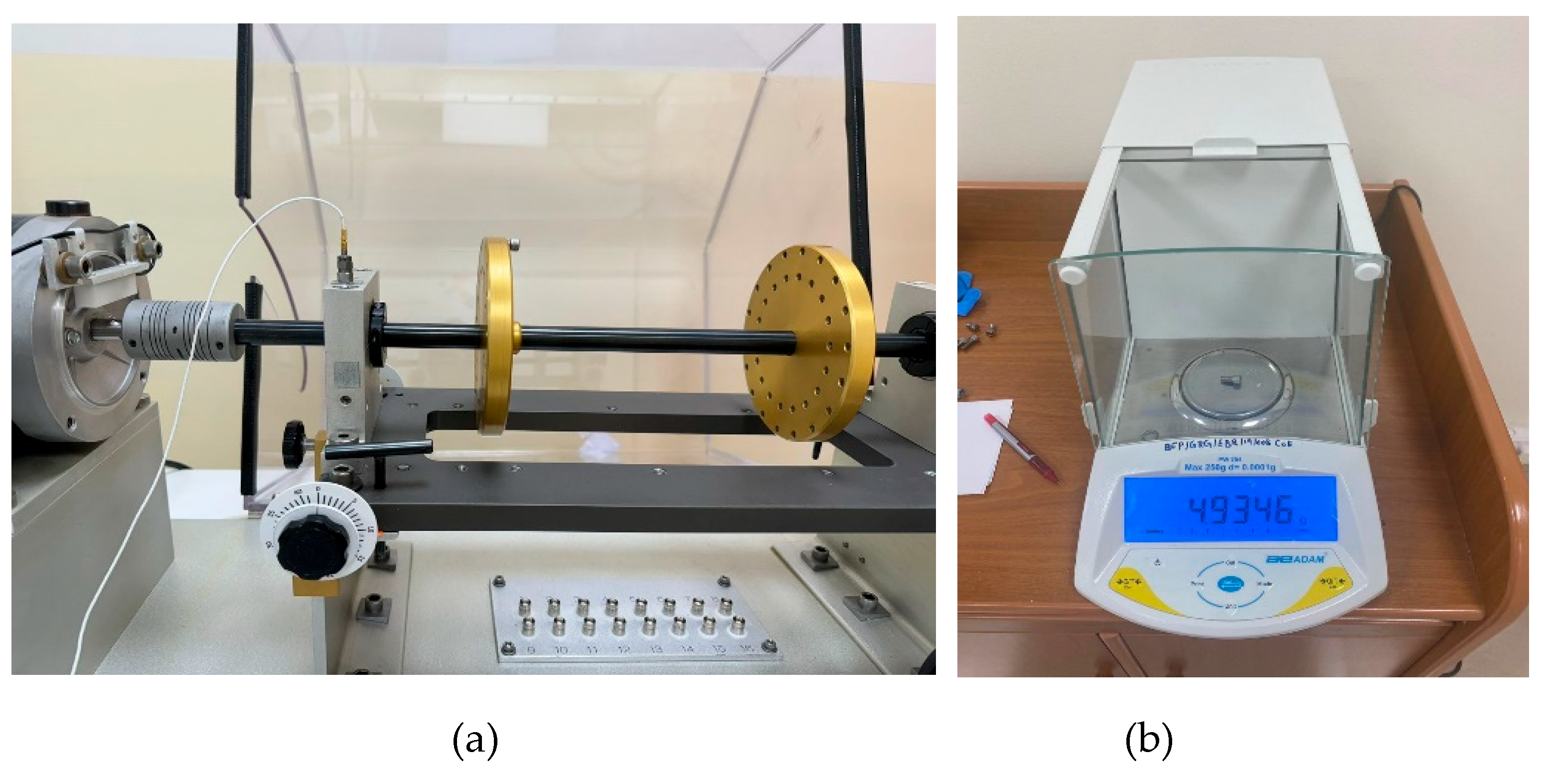
As for the experiment a total of 18 different weights were taken as shown in the
Table 1 and were placed randomly in either the right or left rotary shaft as shown in
Figure 6(a). The accurate weight has been measured with digital weighing machine as shown in
Figure 6(b). The added weights generated distinct vibration signatures in the data, particularly at specific harmonic frequencies. These signatures were analyzed to determine how different imbalances influenced the machine’s operational dynamics.
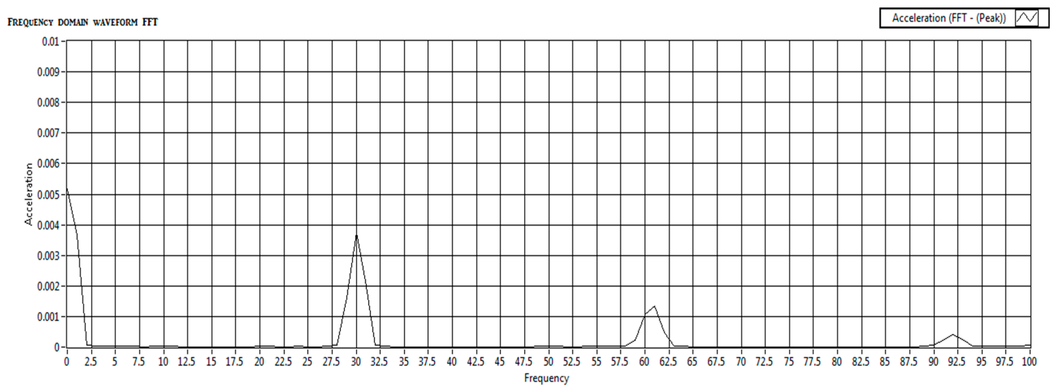
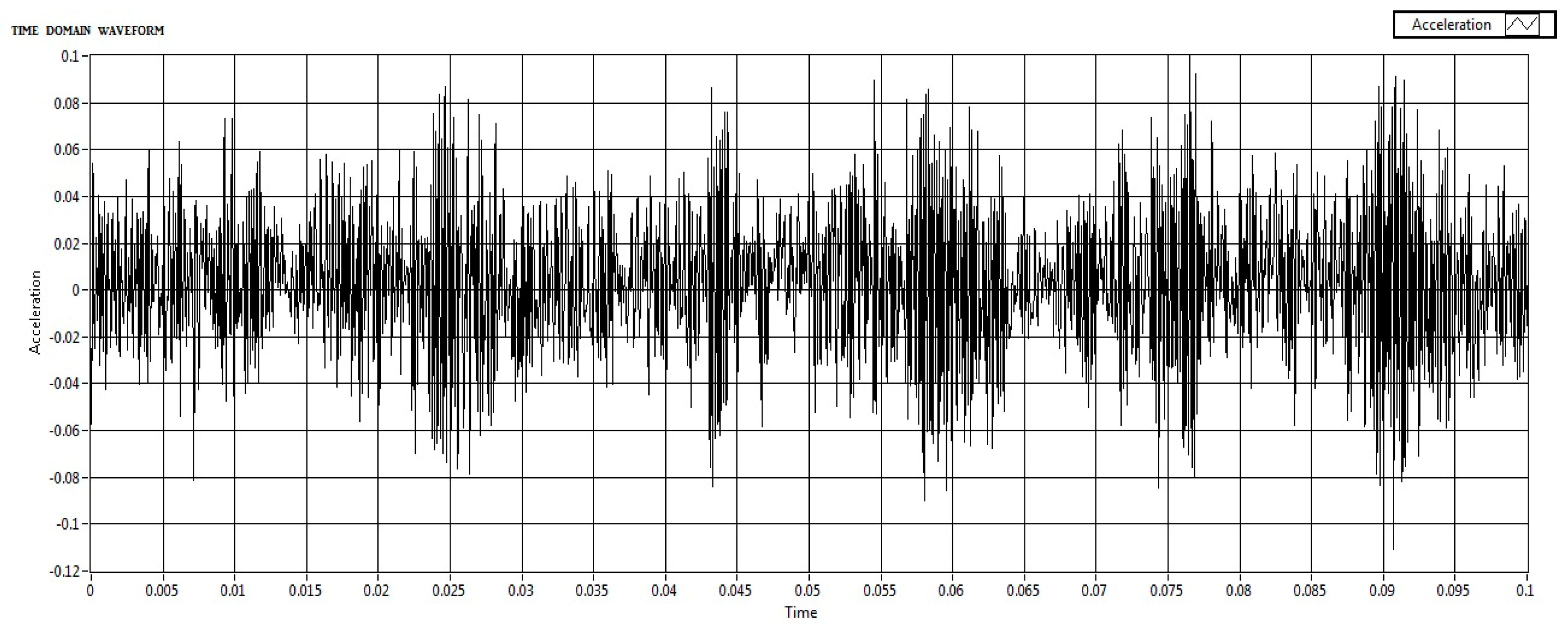
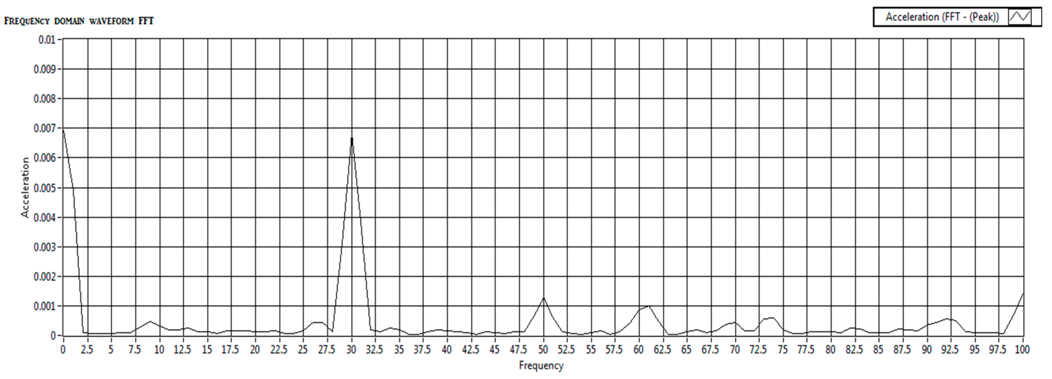
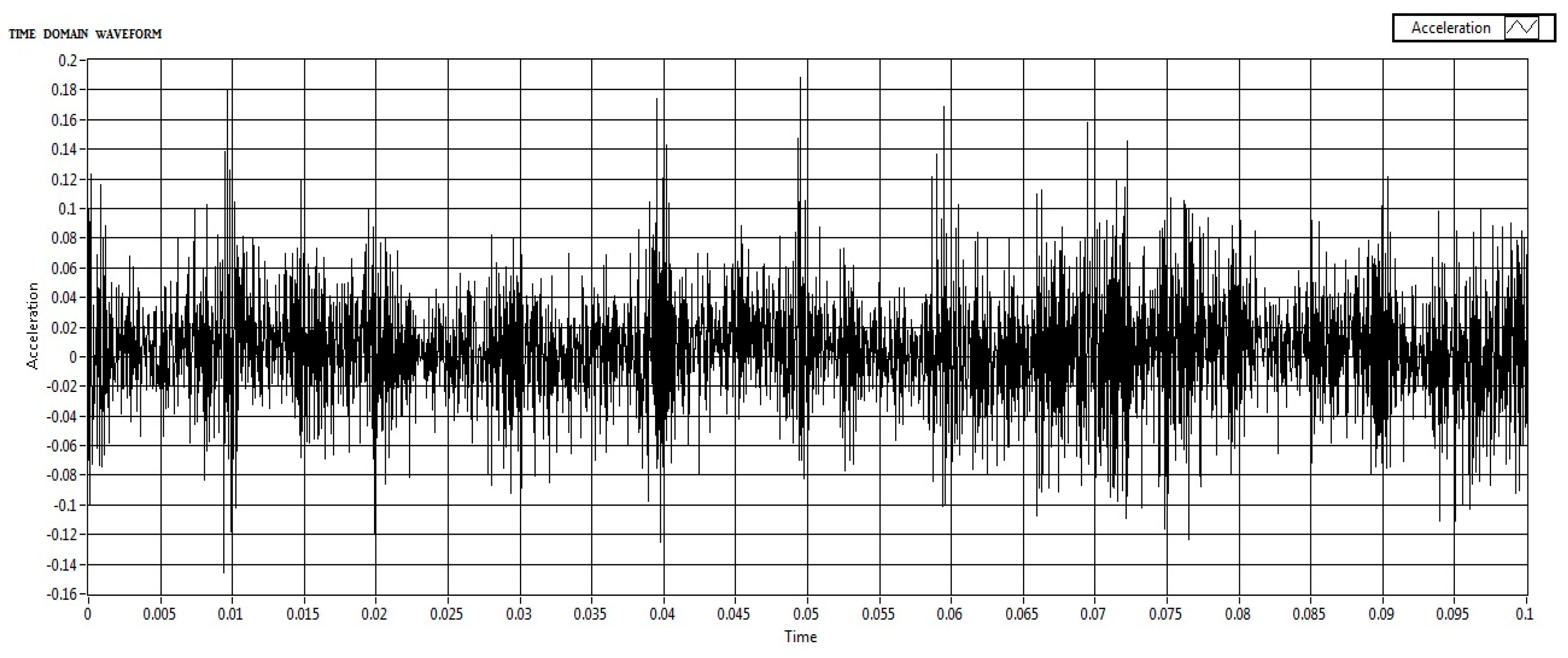
In the signal collection method, National Instruments’ LabVIEW was used to visualize the accelerometer data in real-time by collecting both time and frequency-domain data were collected using the National Instruments devices. Laboratory Virtual Instrumentation Engineering workbench (LabVIEW) is an Instrumentation software in which the acquired signal/data can be stored and analyzed. In this work, NI CDAQ-9174 Which means Data acquisition card and the accelerometer’s signal condition card NI-9234 were used. In the collection of data, the motor was operated at a frequency of 30 HZ and with a gear or shaft frequency of 216 HZ. Data acquisition began only once the motor stabilized at 30Hz to ensure consistent and reliable data. This setup ensured that the data collected was representative and consistent, enhancing the reliability of subsequent analysis. After time and frequency signal collection, both time and frequency domain data are compiled and written to a measurement file. This visual representation helps understand the complete data flow from acquisition to storage, highlighting the parallel processing of time and frequency domain data. Baseline data was recorded from a balanced system with no added weights which are shown in
Figure 7 and
Figure 8.
In the Imbalance Introduction, Screws of different weights were added to the rotary shaft disks to simulate various levels of imbalance and the signals have been collected which are shown in
Figure 9 and
Figure 10.
Both frequency-domain and time-domain acceleration data were captured during each test run. This approach provided a comprehensive dataset for analysis, with a focus on capturing the effects of imbalances through systematic simulations. In this experiment, we focused exclusively on frequency-domain data to detect shaft imbalances in rotating machinery. This decision was driven by the superior ability of frequency-specific responses to indicate shaft imbalances compared to time-domain analysis. Imbalances in rotating machinery manifest as distinct peaks and harmonics within specific frequency ranges, making frequency-domain analysis particularly effective at capturing these characteristics.
By analyzing the frequency domain, we can isolate key features such as resonant frequencies and harmonic distortions that are directly linked to mechanical imbalances. This offers a more precise diagnosis than time-domain analysis alone, as noted by Nossier et al. [
50]. Frequency-domain analysis is a well-established method in mechanical fault detection, supported by both theoretical research and practical applications. Yi et al. highlighted its effectiveness in isolating vibration signals corresponding to specific fault frequencies, which are often indicative of the condition of rotating components. The inherently periodic nature of shaft vibrations makes frequency-domain analysis particularly suited for identifying imbalances in such systems [
51]. As Mali et al., point out, this approach allows for a more targeted examination of the periodic behaviors that are hallmarks of shaft imbalances [
52]. Furthermore, Hertel et al. demonstrated that this method ensures crucial frequency components related to imbalance are emphasized, making the detection process more reliable and accurate under simulated conditions [
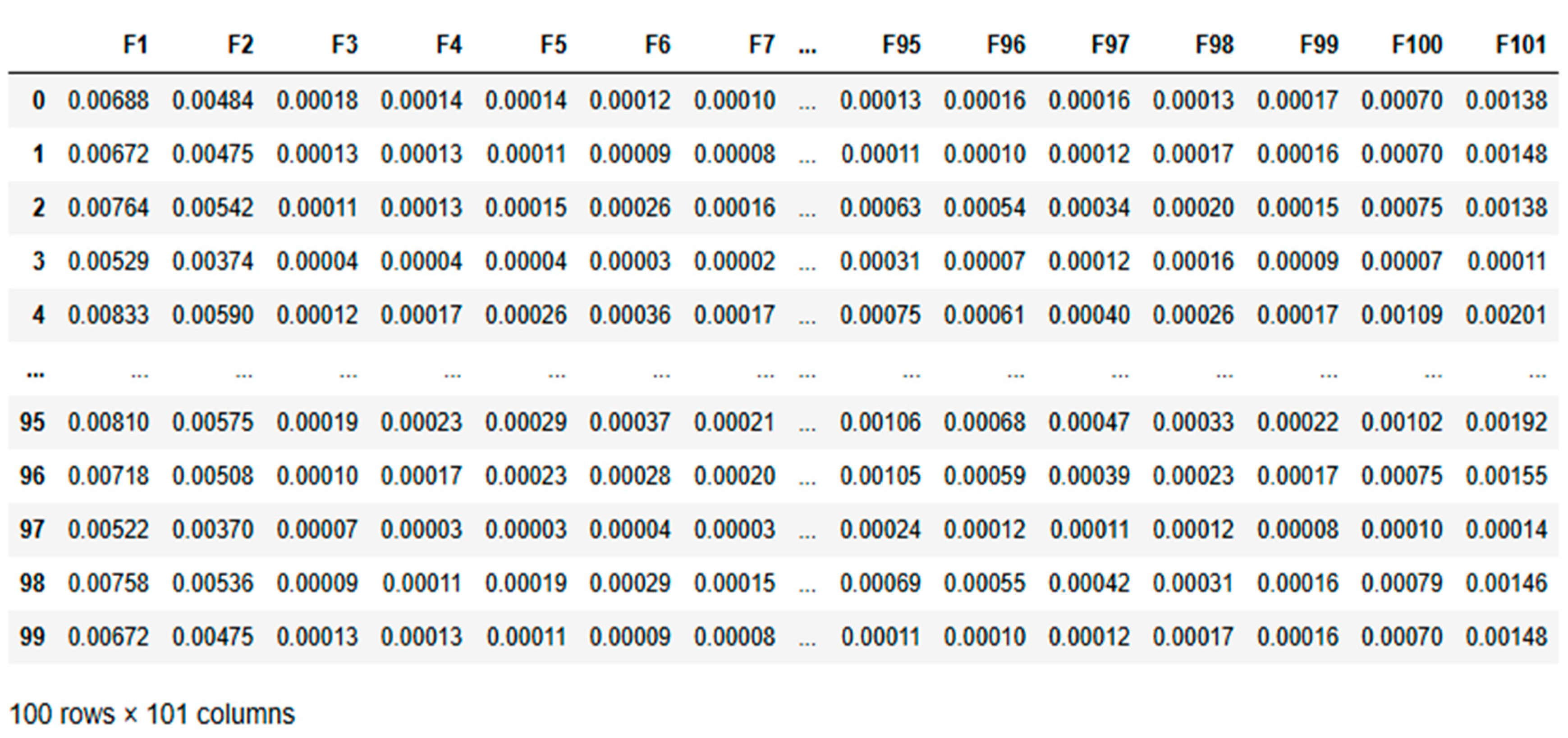
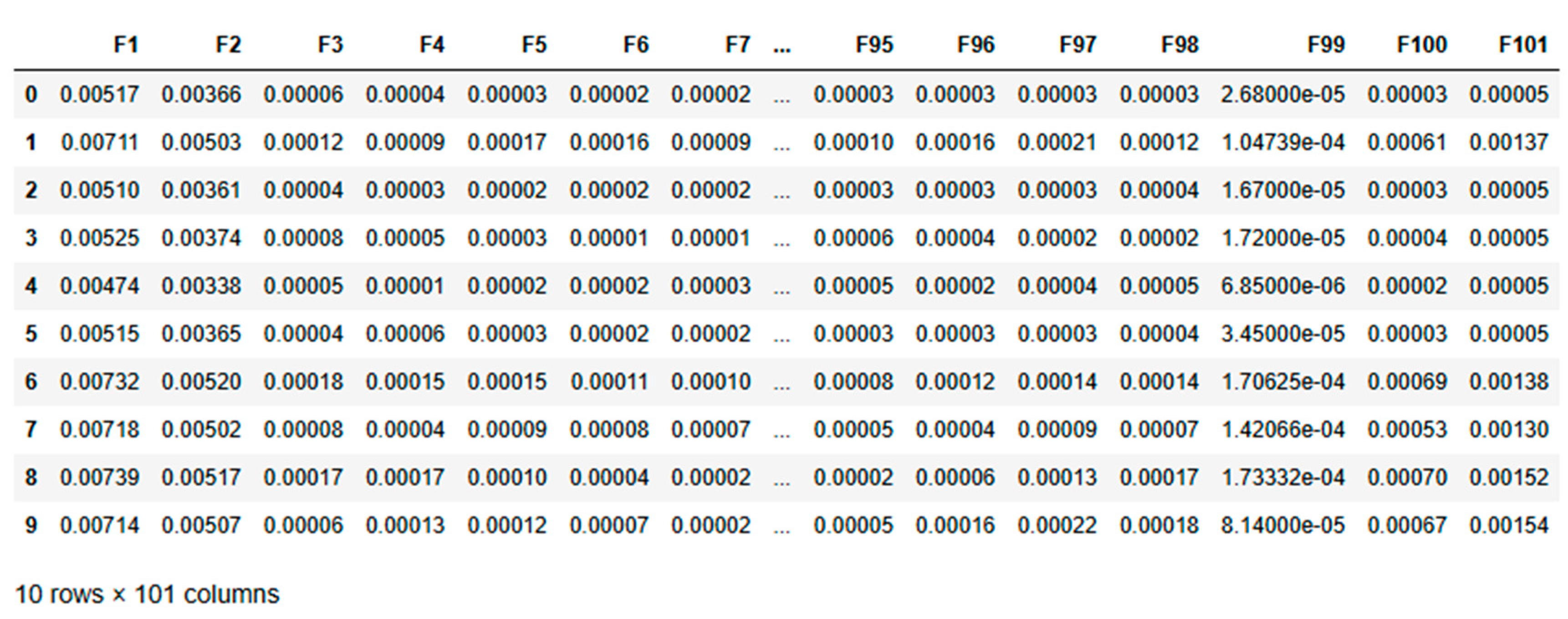
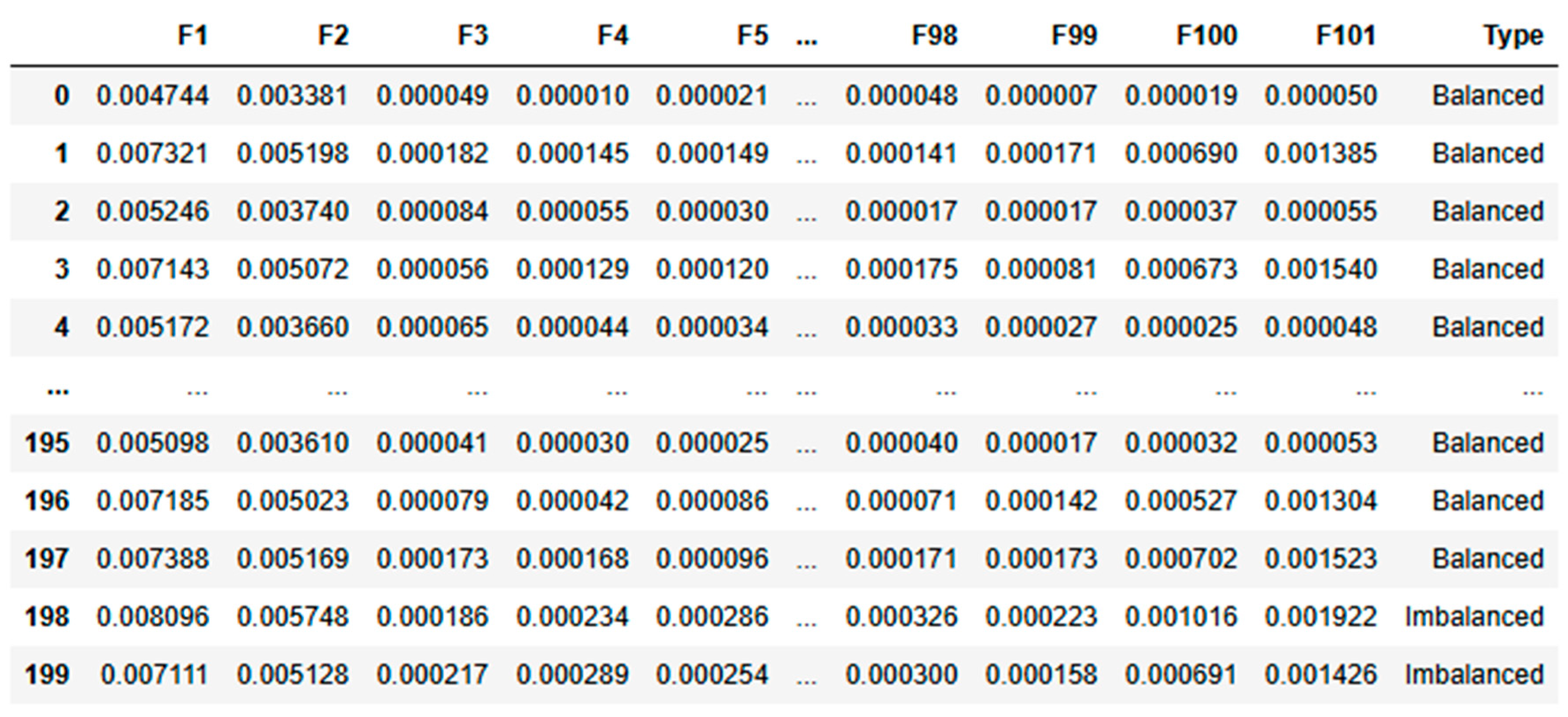
53]. For this experiment, we collected acceleration data for frequencies ranging from 1 to 100 Hz. This dataset shown in
Table 2 and
Table 3 form the basis for training our algorithm to distinguish between balanced and imbalanced conditions. The raw frequency-domain data for both balanced and imbalanced conditions, before any processing is applied, is shown in the following tables:
While frequency-domain analysis offers significant advantages for detecting shaft imbalances, it’s important to note its limitations. Focusing solely on frequency-domain data may miss transient or dynamic features of imbalances that time-domain or wavelet analysis could capture. In practical applications where conditions change rapidly, additional analysis techniques might be required for a comprehensive diagnosis, as suggested by Yan [
54]. This comprehensive setup and data collection process provides a solid foundation for applying deep learning techniques to condition monitoring. By leveraging the strengths of frequency-domain analysis, we aim to develop more accurate and reliable diagnostic models for rotating machinery. The nature of shaft vibrations is inherently periodic, and frequency-domain analysis directly targets this periodicity, making it the preferred choice for identifying imbalances in such systems. This dataset designed for a condition monitoring task and contains 110 entries across 102 columns. It includes 101 numerical features (F1 to F101), which are likely indicative of various measurements relevant to the monitoring process. The final column, “Type,” is a categorical target variable that classifies each entry as either “Imbalanced” or “Balanced.”
The dataset is notably imbalanced, with 100 entries labelled as “Imbalanced” and only 10 as “Balanced.” The numerical features exhibit low mean values, suggesting that the data has likely been standardized or normalized. Although most features show low variability, some have higher standard deviations, indicating varying levels of fluctuation in the monitored parameters.
Kurtosis is a measure of peakedness and hence it is a fine indicator of signal impulsive-ness in fault detection for rotating components especially for drill bits.
Kurtosis is expressed as
Where µ = mean of time series x
σ = standard deviation of time series x
E{.} is the expectation operation
The minus 3 is to make kurtosis of the normal distribution of the normal distribution equal to zero.
So, kurtosis analysis reveals diverse distribution characteristics among the features. For example, features like F1 to F4 have extremely high kurtosis values, potentially indicating the presence of outliers or rare events. In contrast, features such as F97, F98, F100, and F101 exhibit negative kurtosis, implying a more consistent and flat distribution.
The collected data underwent several preprocessing steps to prepare it for input into the deep learning models. These steps were essential in ensuring that the models received data in a format conducive to effective learning. Many research papers are using signal preprocessing techniques such as discrete wavelet transform, wavelet packet transform etc. before implementation of ML and DL algorithms. In this work, it is not mandatory due to the following reasons.
Direct Feature Extraction: The raw data’s inherent characteristics are sufficient for the deep learning models to learn and detect anomalies without additional preprocessing.
Model Robustness: Modern deep learning models are robust enough to handle raw data, reducing the need for extensive preprocessing.
Computational Efficiency: Avoiding complex preprocessing steps can save computational resources and time, making the monitoring system more efficient.
6. Sampling Strategy to Balance Classes
Given the potential imbalance in the data, a sampling strategy was implemented to balance the dataset. This involved oversampling the minority class to ensure that the deep learning models received a balanced dataset. This approach is crucial in preventing the models from becoming biased toward the majority class, leading to more accurate and generalizable predictions.
2. Shuffling:
The dataset was shuffled to randomize the order of the data points. This step prevents the models from learning any order-based biases, which could lead to overfitting and poor generalization to new data.
3. Standardization:
Features were standardized using StandardScaler, a preprocessing technique that transforms the data such that each feature has a mean of 0 and a standard deviation of 1. This process is vital for deep learning models, as it ensures that all features contribute equally to the learning process, avoiding biases toward features with larger numerical ranges.
4. Reshaping:
The data was reshaped to match the input requirements of different deep learning models. For instance:
MLP: The data was formatted into 2D arrays where each row represents a sample, and each column represents a feature.
CNN and LSTM: The data was reshaped into 3D arrays, with dimensions corresponding to the number of samples, timesteps, and features. This reshaping is crucial for CNNs and LSTMs to process spatial and temporal patterns effectively.
5. Data Augmentation via Duplication:
To increase the dataset’s size and improve model robustness, the data was duplicated 2 times and 4 times in separate experiments. This duplication aimed to provide the models with more examples, helping them generalize better to unseen data. However, care was taken to ensure that this augmentation did not introduce redundancy that could lead to overfitting, especially in models like LSTM.
The collected data underwent several preprocessing steps to prepare it for input into the deep learning models, ensuring that the models received data in a format conducive to effective learning which is given in
Table 4. While many research papers use signal preprocessing techniques such as discrete wavelet transform and wavelet packet transform before implementing machine learning and deep learning algorithms [
55], this work found it unnecessary due to several reasons. Firstly, the raw data’s inherent characteristics were sufficient for the deep learning models to learn and detect anomalies without additional preprocessing. Secondly, modern deep learning models are robust enough to handle raw data, reducing the need for extensive preprocessing [
56]. Lastly, avoiding complex preprocessing steps can save computational resources and time, making the monitoring system more efficient.
6. Application of Deep Learning in Condition Monitoring
Deep learning is a branch of machine learning that involves neural networks with multiple layers. It enables the automatic extraction of complex patterns and features from large datasets. These models learn representations directly from raw data through layers of interconnected neurons, making them robust for tasks that involve classification, prediction, and pattern recognition [
57].
In this project, deep learning was employed to analyze frequency-domain data from a rotary shaft for condition monitoring. Deep learning models allowed for automatically detecting imbalances and other faults in the machinery without manual feature engineering. By leveraging deep learning’s ability to handle complex, non-linear data, the models effectively differentiated between balanced and imbalanced states, demonstrating the practical application of these techniques in monitoring conditions based on frequency-domain signals.
6.1. Multilayer Perceptron (MLP)
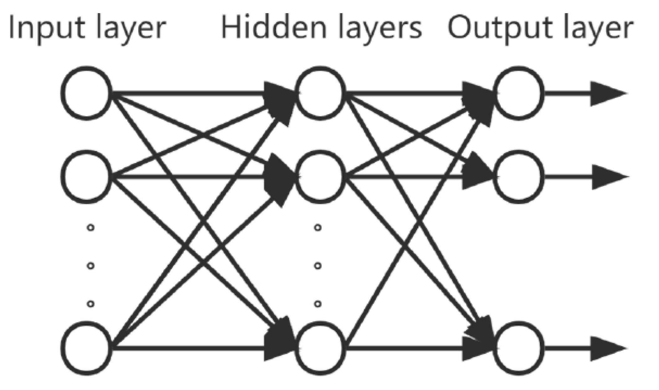
A Multilayer Perceptron (MLP) is a feedforward artificial neural network (ANN) consisting of at least three layers of nodes: an input layer, one or more hidden layers, and an output layer. Each node, or artificial neuron, in one layer, is connected to every node in the next layer with an associated weight. These weights are adjusted during the training process using backpropagation, a supervised learning technique that minimizes the error between the predicted and actual outputs [
58].
A connection between two nodes is assigned a weight value that represents the relationship between them as shown in
Figure 11. In a hierarchical connection, there is a weight property, and the node function can perform both summation and activation operations.
The summation function is
where is the amount of input data, is the input data, is the deviation, and is the connection weight.
The output is obtained in the hidden layer using the activation function as
The output of the output layer cell in the MLP can be obtained by combining Equations (1) and (2)
MLPs are particularly effective for tasks where the relationship between input features and output labels is complex but does not involve spatial or temporal dependencies. They are widely used in applications such as pattern recognition, classification, and regression [
59].
6.2. Convolutional Neural Network (CNN)
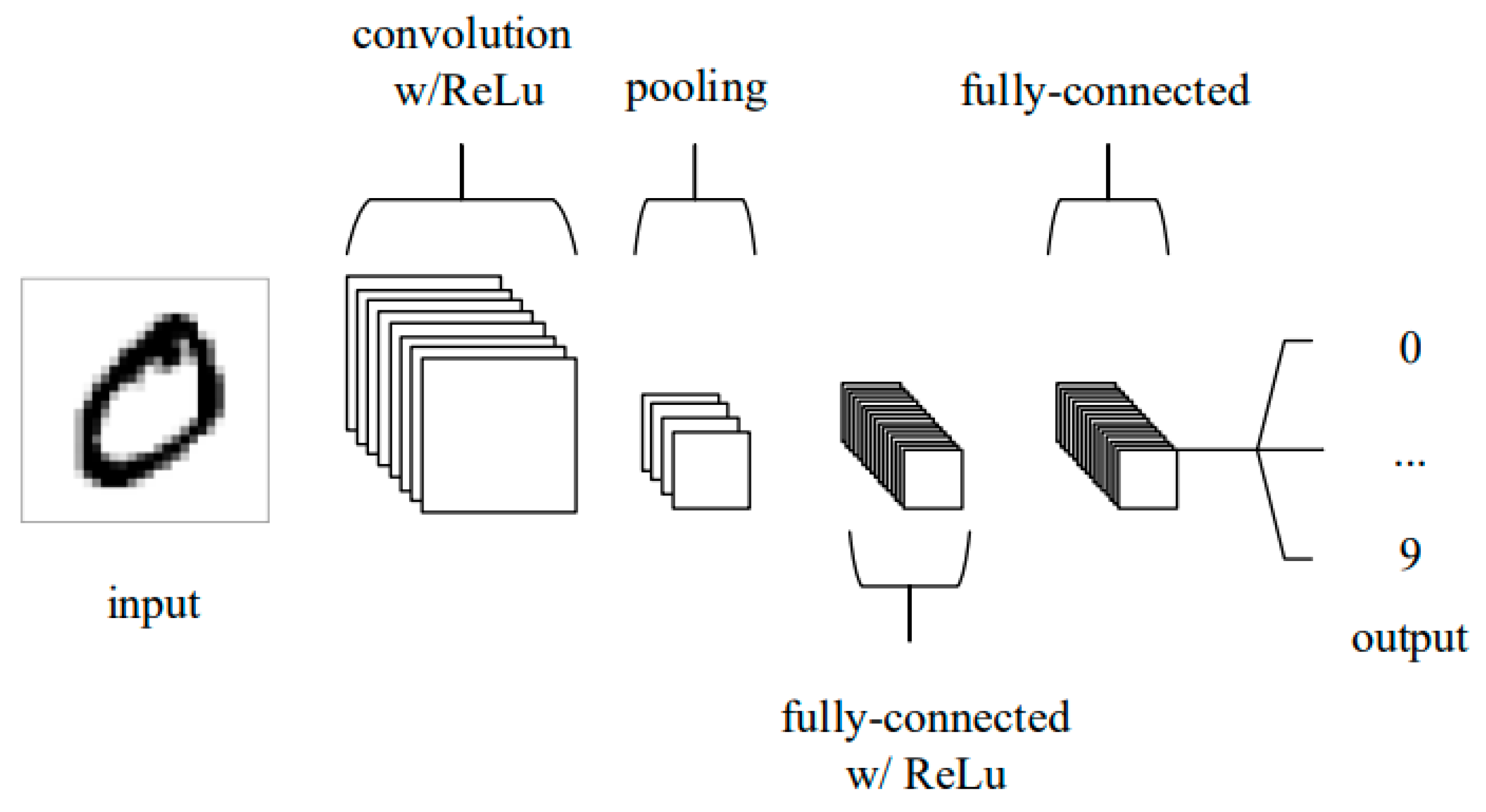
A Convolutional Neural Network (CNN) is a type of deep neural network designed to process data with a grid-like structure, such as images. CNNs utilize convolutional layers that apply filters to the input data, identifying local patterns like edges and textures. These features are then aggregated and classified by fully connected layers. CNNs are highly effective in image recognition tasks due to their capability to capture spatial hierarchies in data [
60].
These networks have revolutionized computer vision tasks, achieving unprecedented performance in image classification, object detection, and various signal processing application [
61].
At the heart of CNNs lies the convolution operation, from which they derive their name as shown in
Figure 12.
This mathematical operation enables the network to capture local patterns and spatial hierarchies within input data. In the context of image processing, the discrete convolution operation can be expressed as:
Explanation:
(S (i, j)) is the output of the convolution operation at position ((i, j)).
(I) is the input matrix.
(K) is the kernel (filter) matrix.
((i, j)) are the coordinates of the output matrix.
((m, n)) are the coordinates of the input matrix.
This formula represents the convolution operation, where the kernel (K) is applied to the input (I ) to produce the output ( S ). For each position ((i, j)) in the output matrix, the value is computed by summing the products of the overlapping elements of the input matrix and the kernel [
62].
The architecture of a CNN typically comprises several specialized layers:
Convolutional layers apply filters to the input data, detecting local patterns.
Activation layers introduce non-linearity. A common activation function is the Rectified Linear Unit (ReLU):
Pooling layers reduce spatial dimensions. Max pooling, a common operation, can be expressed as:
Where R_i,j represents a local neighborhood around position (i,j)[
63].
Fully connected layers perform final classification based on extracted features:
Here , is an activation function, are weights, are inputs, and b is a bias term.
The learning process in CNNs is facilitated by backpropagation, adjusting network parameters to minimize error. The weight update rule can be expressed as:
Where
is the learning rate and E is the error function [
61].
CNNs offer several advantages over traditional neural networks in image processing tasks. They employ parameter sharing and local connectivity, significantly reducing the number of learnable parameters. These properties, combined with translation invariance, make CNNs exceptionally effective in capturing spatial hierarchies in visual data [
57].
The power of CNNs lies in their ability to automatically learn hierarchical representations. As data progresses through the network, it transforms from raw pixel values to increasingly abstract features. This hierarchical learning enables CNNs to capture intricate patterns within images, often surpassing human-level accuracy in specific visual recognition tasks [
63].
CNNs represent a significant advancement in machine learning and artificial intelligence, particularly in computer vision. Their unique architecture, built upon convolution and non-linear activations, enables effective processing of grid-like data structures. As research progresses, CNNs continue to shape the future of AI and its applications across various domains.
6.3. Recurrent Neural Network (RNN) with
Recurrent Neural Networks (RNNs) are a class of neural networks where connections between nodes form a directed graph along a sequence, allowing them to maintain a memory of previous inputs. It means RNN is a special type of artificial neural network adapted to work for time series data or data that involves sequences. RNN can be used Language translation, Speech recognition, Time series forecasting, Text generation, Sentiment analysis etc.
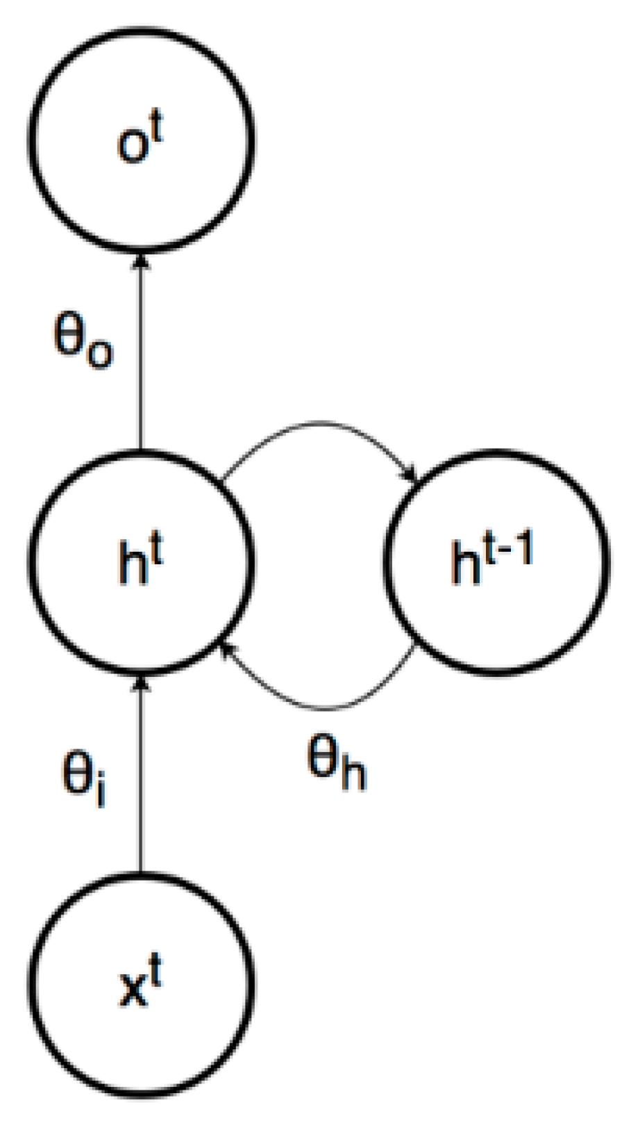
In the
Figure 13 the values of θi, θh, and θo represent the parameters associated with the inputs, previous hidden layer states, and outputs
The following equations define how an RNN evolves over time
where O
t is the output of the RNN at time t, x
t is the input to the RNN at time t, and ℎ
t is the state of the hidden layer(s) at time t. The image below outlines a simple graphical model to illustrate the relation between these three variables in an RNN’s computation graph.
The equation 9 says that, the given parameters
, the output at time
depends on the hidden layer at time
, same like a feedforward neural network. The second equation says that, for the given parameters
, the hidden layer at time
depends on the hidden layer at time
and the input at time
. Originally, the equation 10 demonstrates that the RNN can remember its past by allowing past computations
to influence the present computations
. The aim of training the RNN is to get the sequence
to match the sequence
, where
represents the time lag (it’s possible that
) between the first meaningful RNN output
and the first target output
. A time lag is sometimes introduced to allow the RNN to reach an informative hidden state
before it starts producing elements of the output sequence [
64].
6.4. Long Short-Term Memory (LSTM)
Long Short-Term Memory (LSTM) units are a special kind of RNN designed to capture long-term dependencies in sequential data by incorporating memory cells that can store information across time steps. LSTMs overcome the vanishing gradient problem that affects standard RNNs, making them more effective in learning long-term dependencies [
65]. LSTM have 3 gates: (i)Input Gate (ii) Forget Gate and (ii) Output Gate
Gates in LSTM are the sigmoid activation functions which means the output value between 0 and 1 in which 0 means gates are blocking and 1 means gates are allowing. The gate comprises a sigmoid
neural network layer. Equations for the gates are given as follows
represents input gate.
represents forget gate.
represents output gate.
represents sigmoid function.
weight for the respective gate( ) neurons.
output of the previous lstm block(at timestamp ).
input at current timestamp.
biases for the respective gates .
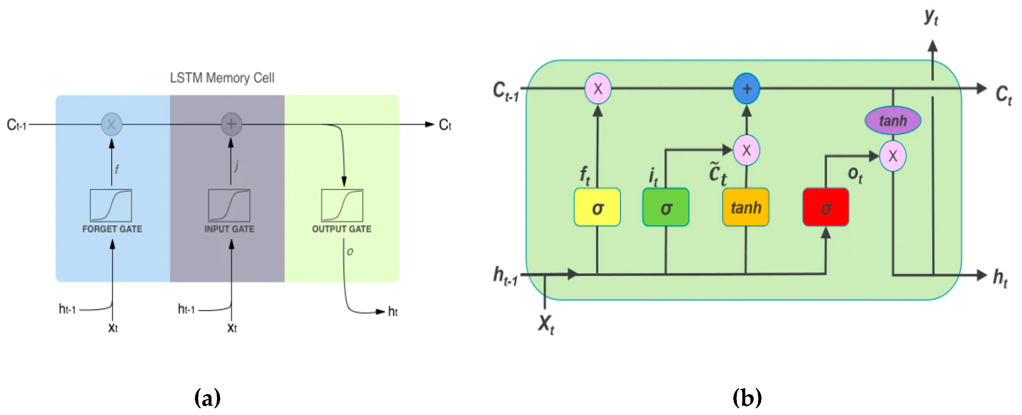
Input Gate equation which tells that what new information will be stored in the cell state. Second Equation is for the forget gate which is used to throw the information away from the cell state. Third one is the output gate which provide the activation to the final output of the LSTM block at timestamp ‘t’ as shown in
Figure 14.
The equations for the cell state, candidate cell state and the final output:
cell state(memory) at timestamp .
represents candidate for cell state at timestamp .
note* others are same as above.
To get the memory vector for the current timestamp (c_{t}) the candidate is calculated. Now, the cell state knows that what it needs to forget from the previous state (i.e f_{t} * c_{t-1}) and what it needs to consider from the current timestamp (i.e i_{t} * c`_{t}). Filtering in the cell state and then it is passed through the activation function which predicts what portion should appear as the output of current LSTM unit at timestamp t. Let’s look at a block of LSTM at any timestamp {t}. We can pass this h_{t} the output from current LSTM block through the softmax layer to get the predicted output(y_{t}) from the current block as shown in
Figure 14.
LSTMs are particularly useful for tasks involving sequential data, such as time series forecasting, natural language processing, and speech recognition. Their ability to retain information over long periods makes them ideal for modeling sequences where the order and duration of events are essential [
67].
6.4. Experimental Design for Deep Learning
Before delving into the detailed comparison of results, it is essential first to explain the rationale behind the experimental setup, which involves evaluating the models across three sections—one with the original data, one with doubled data, and one with quadrupled data.
This structure is designed to assess how well different deep learning models (MLP, CNN, RNN, LSTM) perform with varying data volumes, with the primary goals being to:
Evaluate Model Scalability: Testing with increased data allows us to observe how effectively each model scales as the dataset size grows. Some models may perform better with small datasets but struggle as the data volume increases, while others might improve in performance with more data.
Analyse Generalization and Overfitting: By comparing the training and validation accuracy and loss across different dataset sizes, we can identify whether a model is overfitting (performing well on training data but poorly on validation data) or generalizing well to new, unseen data.
Test Model Stability: Larger datasets can reduce the effect of noise and randomness, leading to smoother learning curves. This comparison helps determine which models remain stable and consistent under varying conditions.
To assess the impact of data scaling on model performance, the dataset was processed in three distinct variations: original, doubled, and quadrupled. This approach allows us to evaluate how each model adapts as the complexity and volume of data increase:
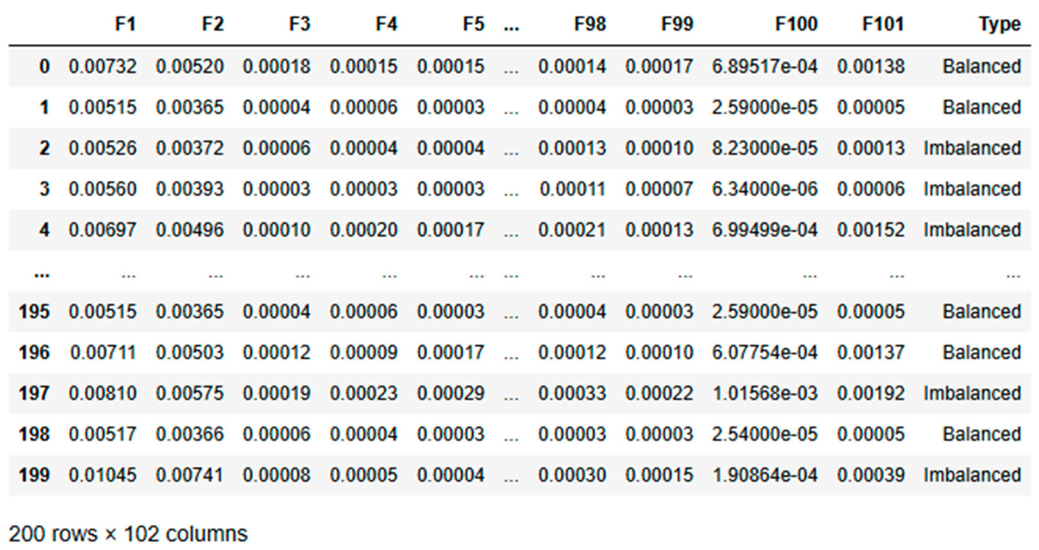
Original Data: This baseline comparison focuses on the model’s performance with the original dataset given in
Table 5. The results provide insight into how well the model can learn patterns from the initial data configuration.

Table 5.
Original dataset.
Table 5.
Original dataset.
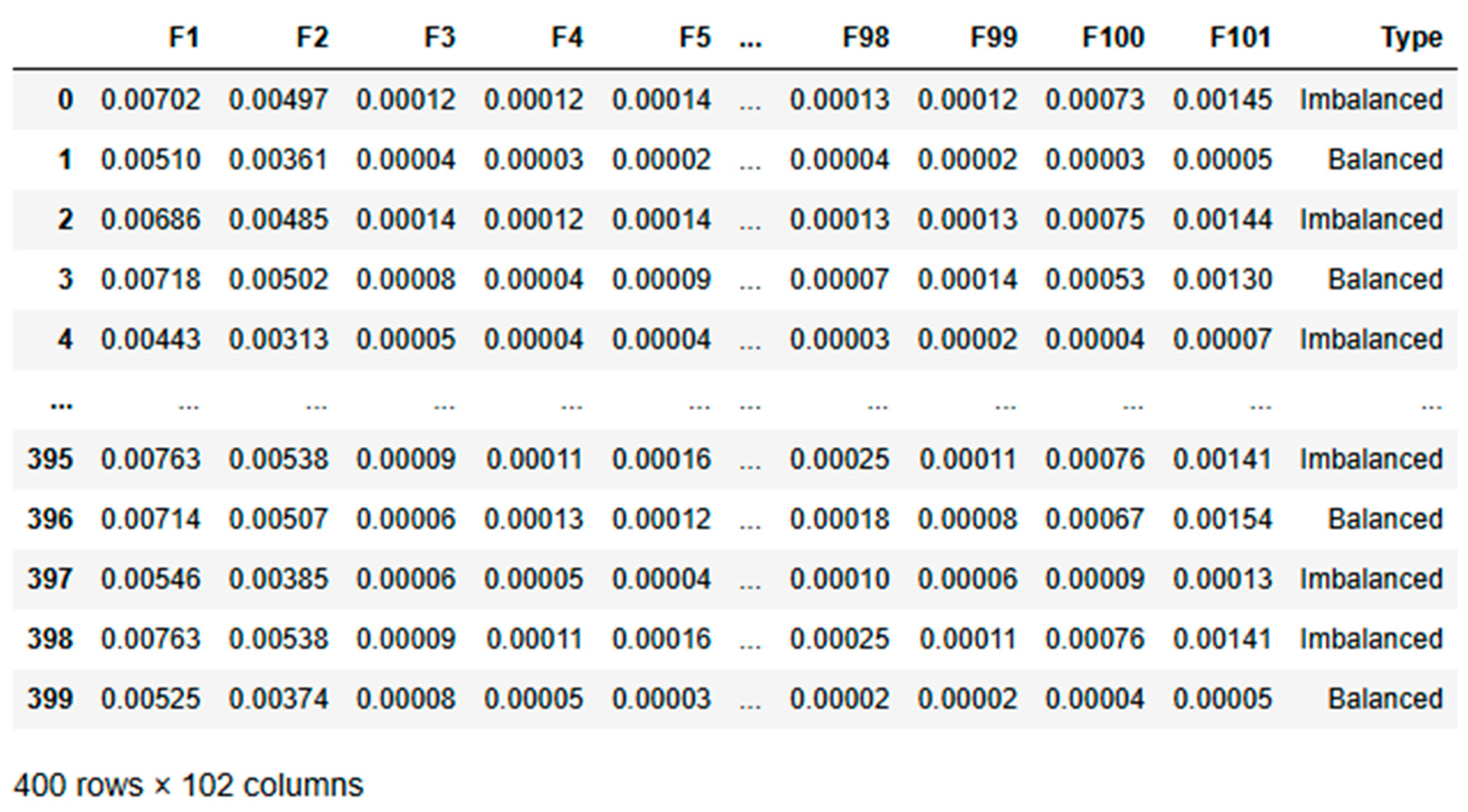
Doubled Data: The dataset is artificially increased by duplicating the data to simulate a scenario with more data available given in
Table 6. This approach simulates a scenario with more data, helping assess how model performance changes with larger datasets.

Table 6.
Doubled dataset.
Table 6.
Doubled dataset.
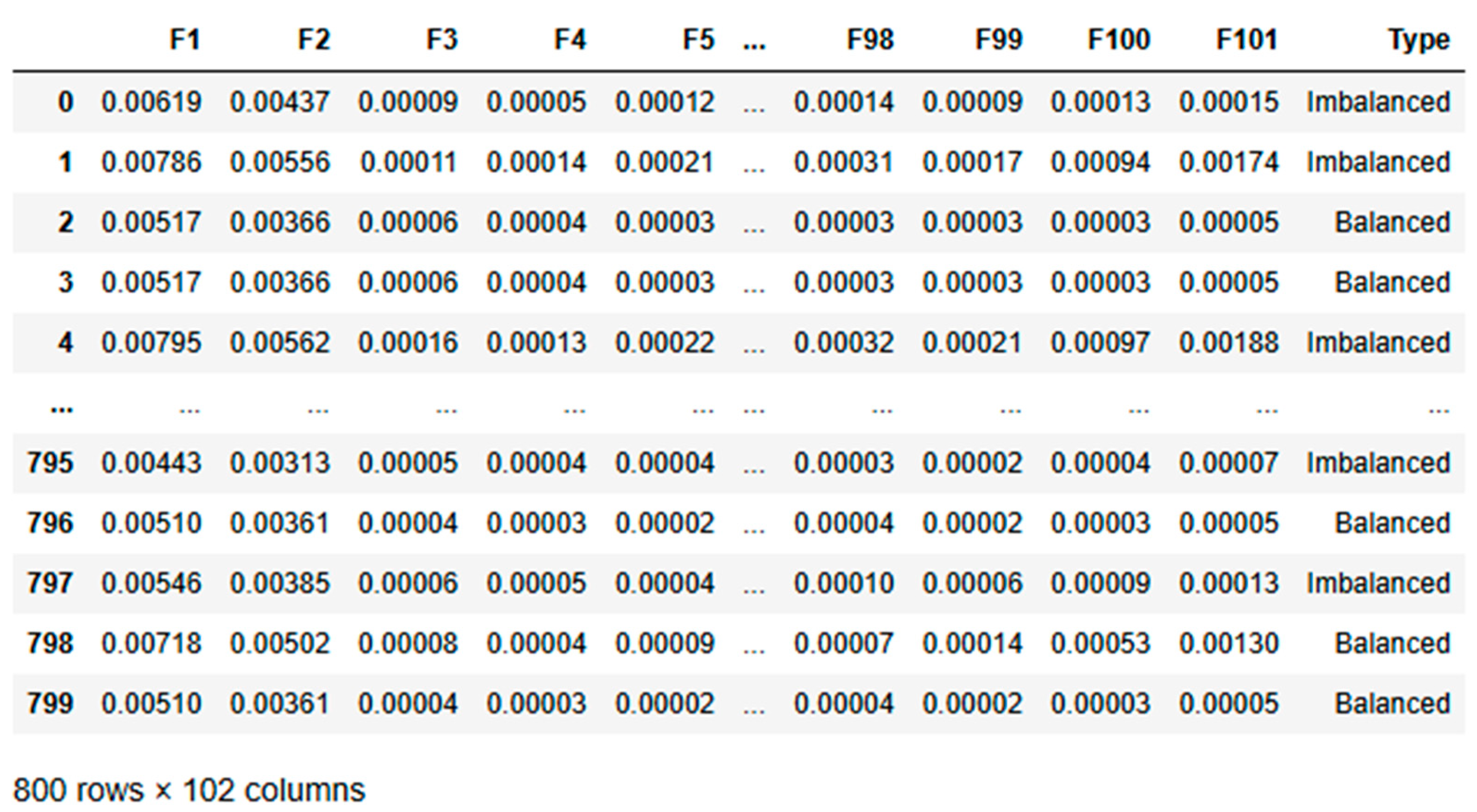
Quadrupled Data: Quadrupling the dataset given in
Table 7 tests the model’s behaviour under even larger data volumes. The results highlight whether the model continues to improve, stabilizes, or begins to exhibit issues such as overfitting.

Table 7.
Quadrupled dataset.
Table 7.
Quadrupled dataset.
6.6. Observations on Model Performance Across Scaled Datasets
The following subsections break down the performance of each model based on different dataset scales:
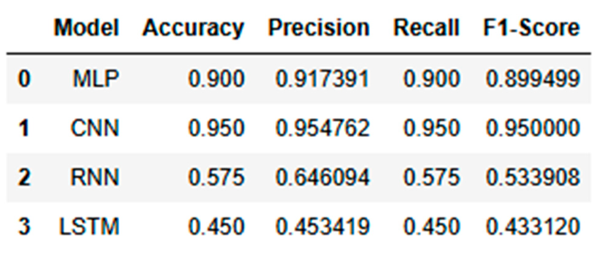
This subsection evaluates each model’s performance using the original dataset, focusing on key metrics like accuracy, precision, recall, and F1-score as shown in
Table 8.
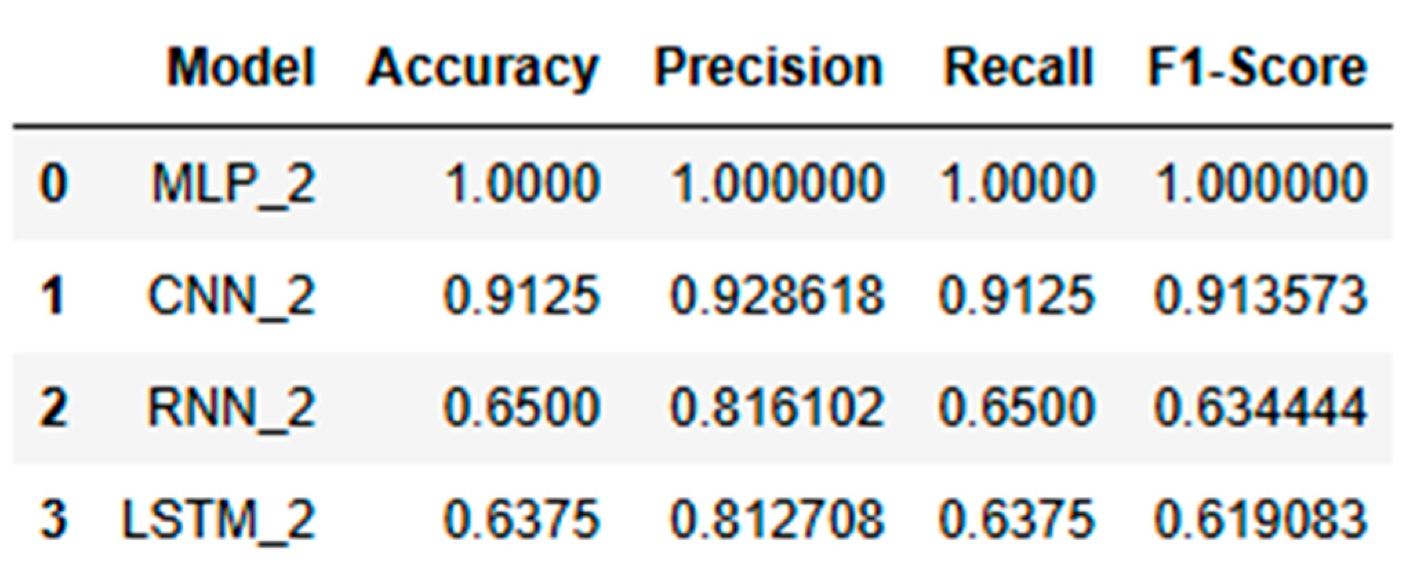
Model Performance for the Doubled Dataset:
In this section, the dataset is doubled in size to analyse whether the increased volume affected the learning capability and generalization of each model. The performance metrics are compared with the normal dataset to identify changes as shown in
Table 9.
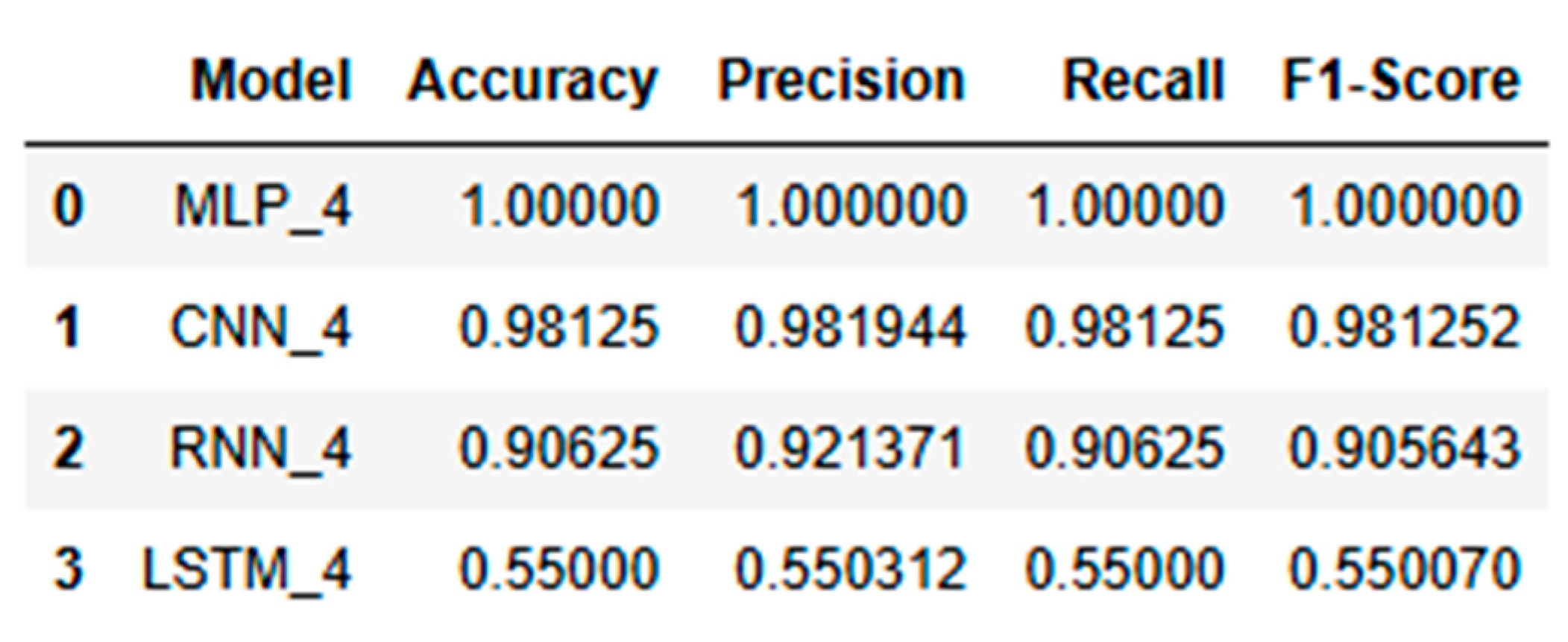
Model Performance for the Quadrupled Dataset:
The dataset size was quadrupled to assess how each model handles a significant increase in data volume and complexity. The metrics given
Table 10 are reviewed to determine whether models can effectively scale and maintain robust performance.
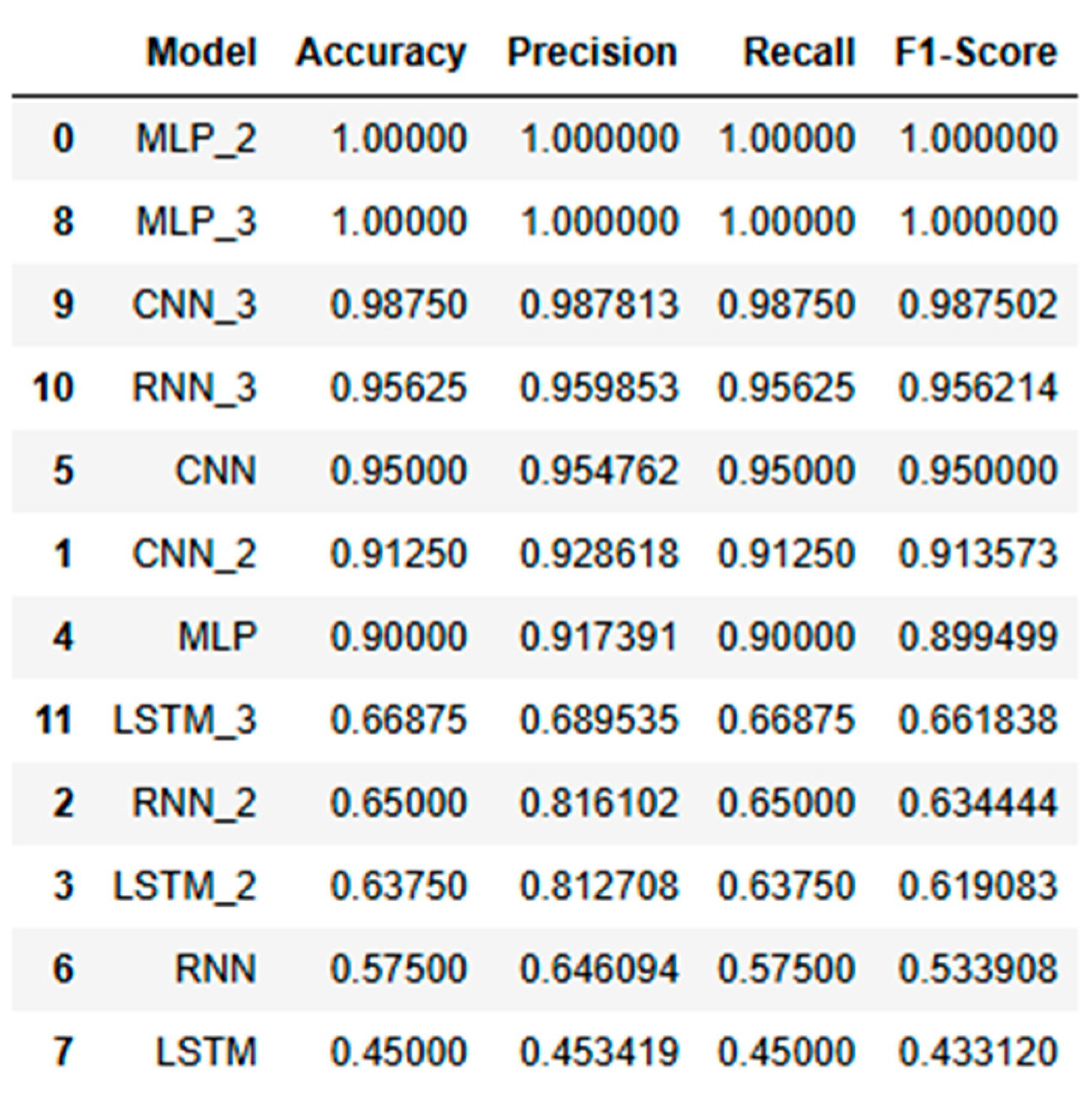
6.7. Rankig the Performance of All AI Models
This section ranks the models based on their overall performance across all datasets, considering the consistency of accuracy, precision, recall, and F1-score as provided in
Table 11. The comparative analysis highlights that models like MLP and CNN adapted well to data scaling, consistently maintaining high accuracy and stable learning, while RNN and LSTM struggled with larger datasets. The ranking of the models based on their scalability and stability underscores the adaptability of certain models over others when faced with increasing data complexity.
7. Comparison between MLP, CNN and RNN and Its Analysis
1. Multilayer Perceptron
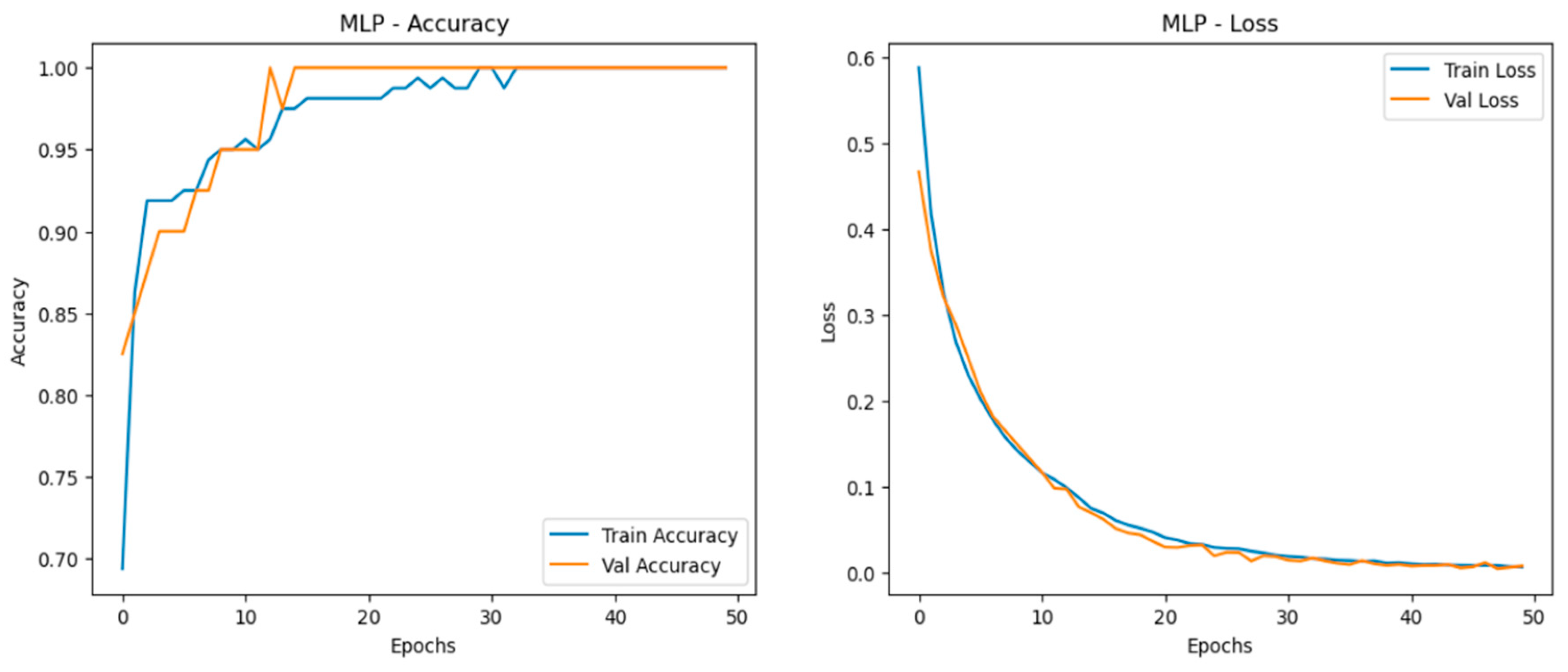
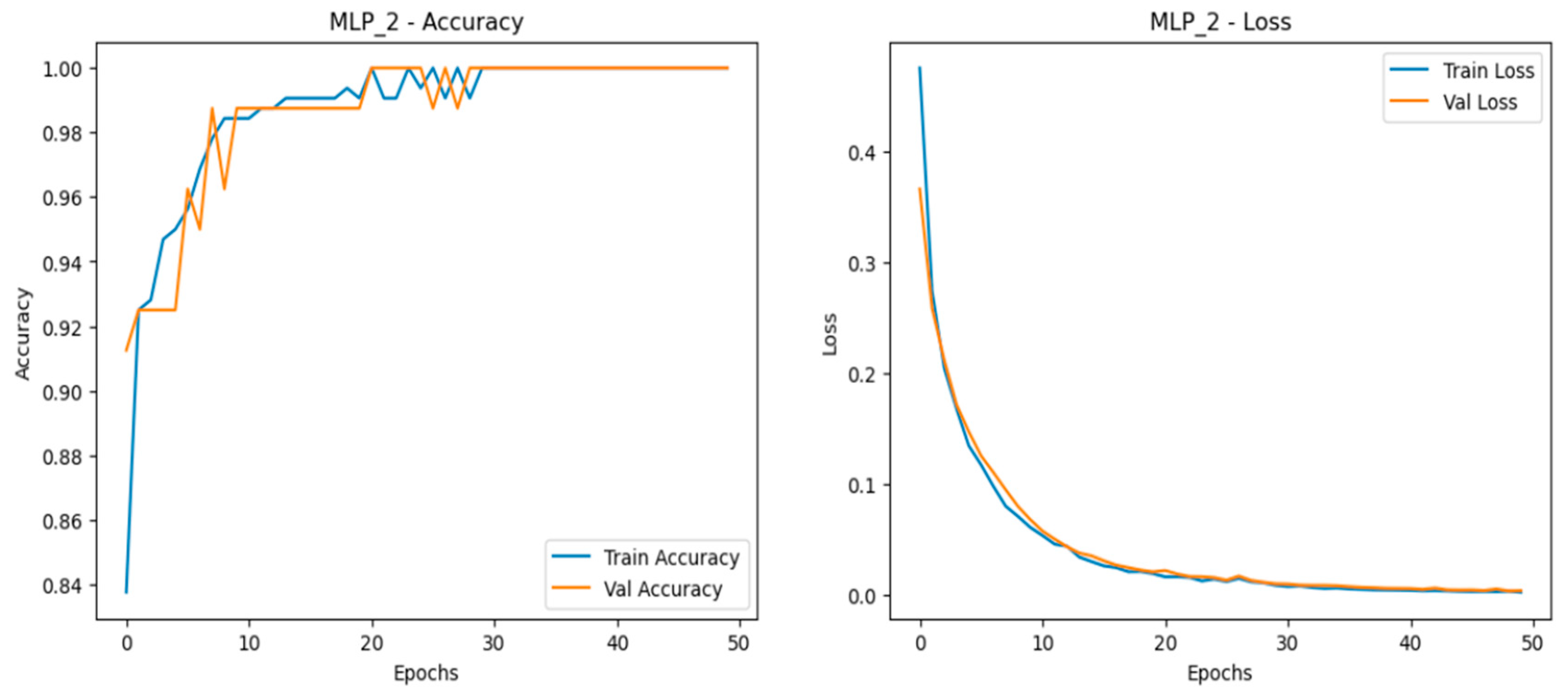
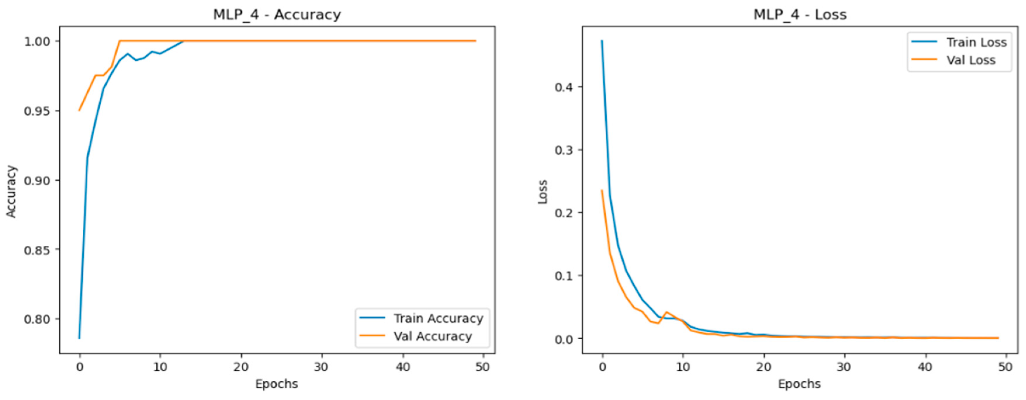
The Multilayer Perceptron (MLP) model consistently delivered near-perfect performance across all scaled datasets—normal, doubled, and quadrupled as shown in
Figure 15,
Figure 16 and
Figure 17.This consistency is reflected in the model’s high accuracy, precision, recall, and F1-score across all scales, making it the most reliable and stable model for this application. The accuracy curves demonstrate close alignment between training and validation sets, indicating strong learning capability with minimal overfitting. The loss curves decrease smoothly and converge closely in all three dataset variations, highlighting effective learning and robustness. Among the datasets, the quadrupled set (MLP_4) performed best, achieving near-perfect accuracy with smoothly converging loss curves, reinforcing the model’s capacity for scalable, stable performance.
- 1.
Normal Dataset
Figure 15.
Training and validation metrics for MLP normal dataset.
Figure 15.
Training and validation metrics for MLP normal dataset.
- 2.
Doubled Dataset
Figure 16.
Training and validation metrics for MLP dataset doubled.
Figure 16.
Training and validation metrics for MLP dataset doubled.
- 3.
Quadrupled Dataset
Figure 17.
Training and validation metrics for MLP dataset quadrupled.
Figure 17.
Training and validation metrics for MLP dataset quadrupled.
2. CNN (Convolutional Neural Network)
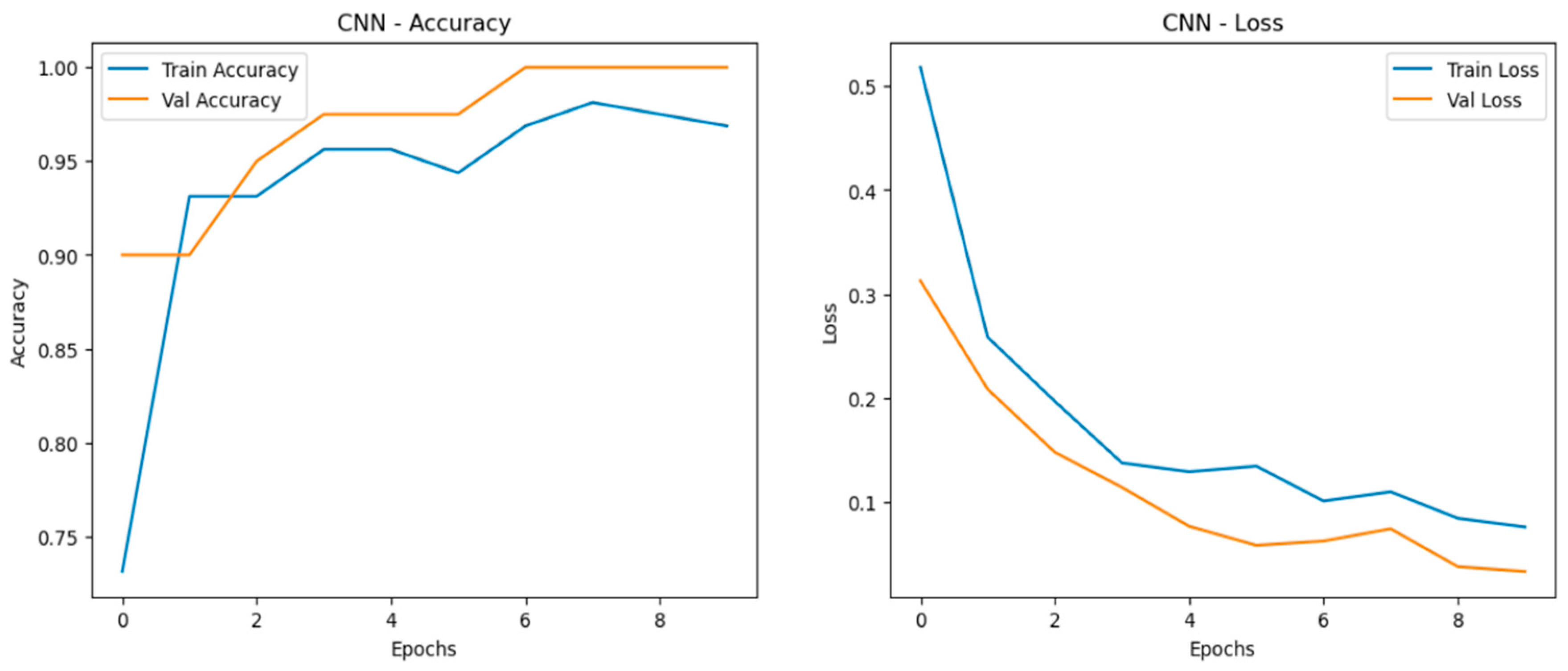
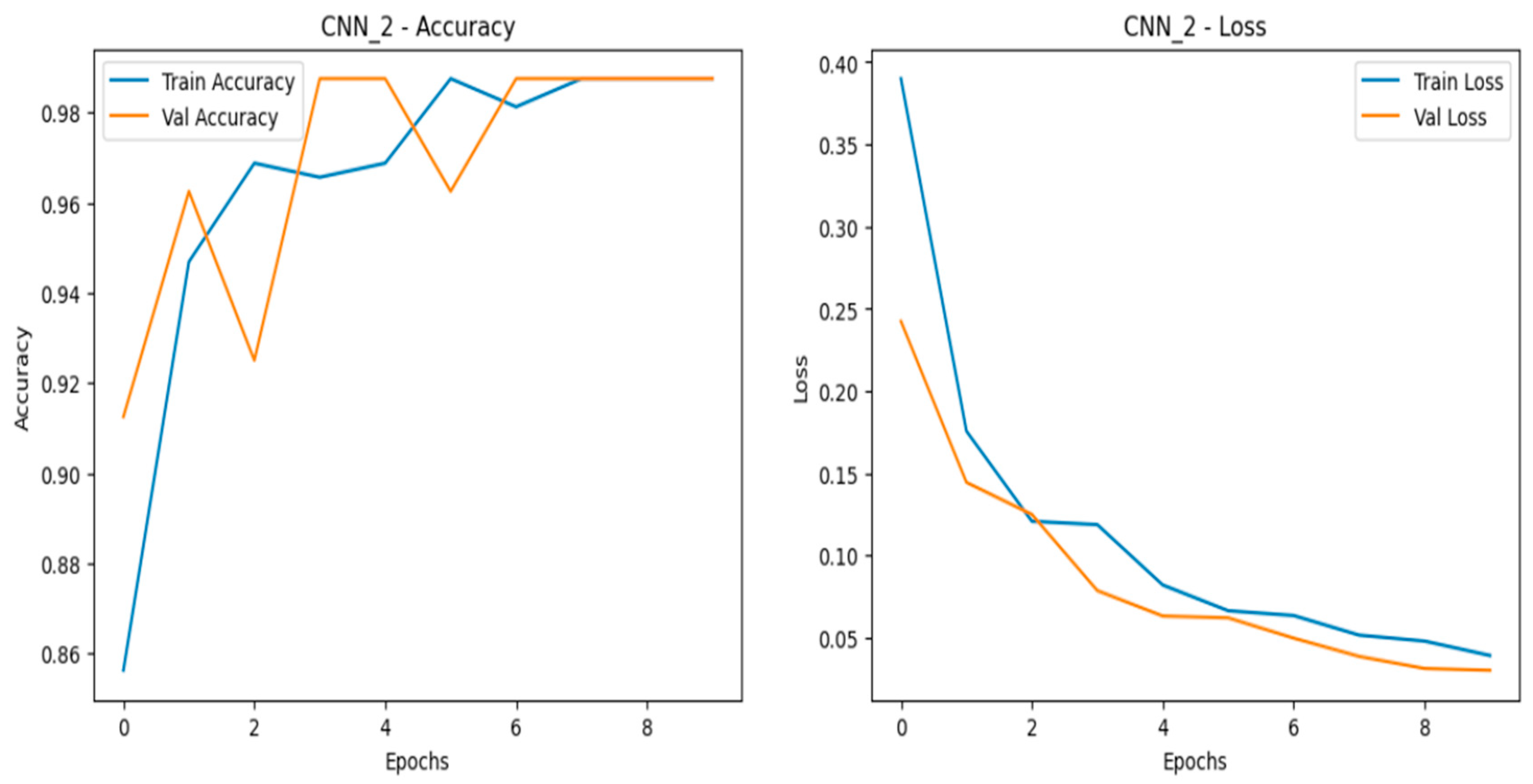
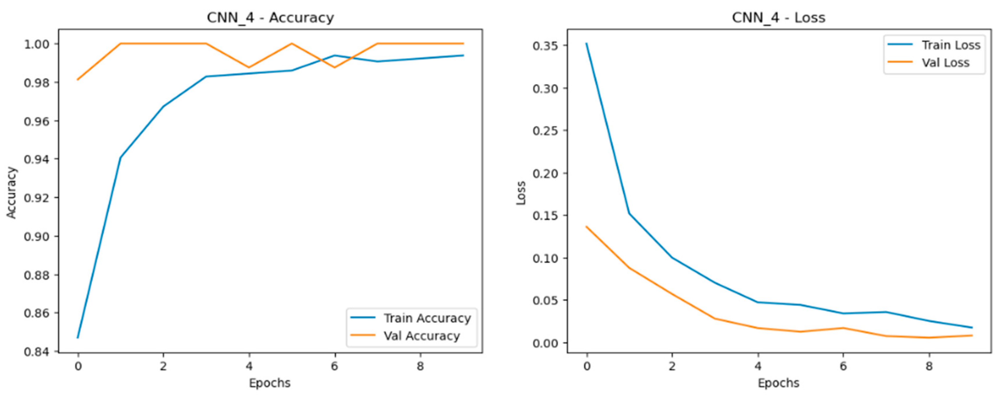
The Convolutional Neural Network (CNN) models performed exceptionally well across all scaled datasets—normal, doubled, and quadrupled—showing only slight variations in performance while maintaining strong accuracy and convergence as shown in
Figure 18,
Figure 19 and
Figure 20. The CNN models demonstrated robust adaptability as data was scaled, with closely aligned training and validation accuracy curves that stabilized early across all datasets. This indicates strong generalization and effective learning. The loss curves consistently decreased and converged smoothly, reflecting minimal overfitting. Among the datasets, the doubled dataset (CNN_2) stood out as the best, with smooth accuracy curves and well-converged loss curves, striking an ideal balance between learning speed and stability. Notably, the CNN_4 model in the quadrupled dataset performed very closely to the MLP, showcasing CNN’s ability to maintain high performance under larger data volumes.
- 1.
Normal Dataset
Figure 18.
Training and validation metrics for CNN normal dataset.
Figure 18.
Training and validation metrics for CNN normal dataset.
- 2.
Doubled Dataset
Figure 19.
Training and validation metrics for CNN dataset doubled.
Figure 19.
Training and validation metrics for CNN dataset doubled.
- 3.
Quadrupled Dataset
Figure 20.
Training and validation metrics for CNN dataset quadrupled.
Figure 20.
Training and validation metrics for CNN dataset quadrupled.
3. RNN (Recurrent Neural Network)
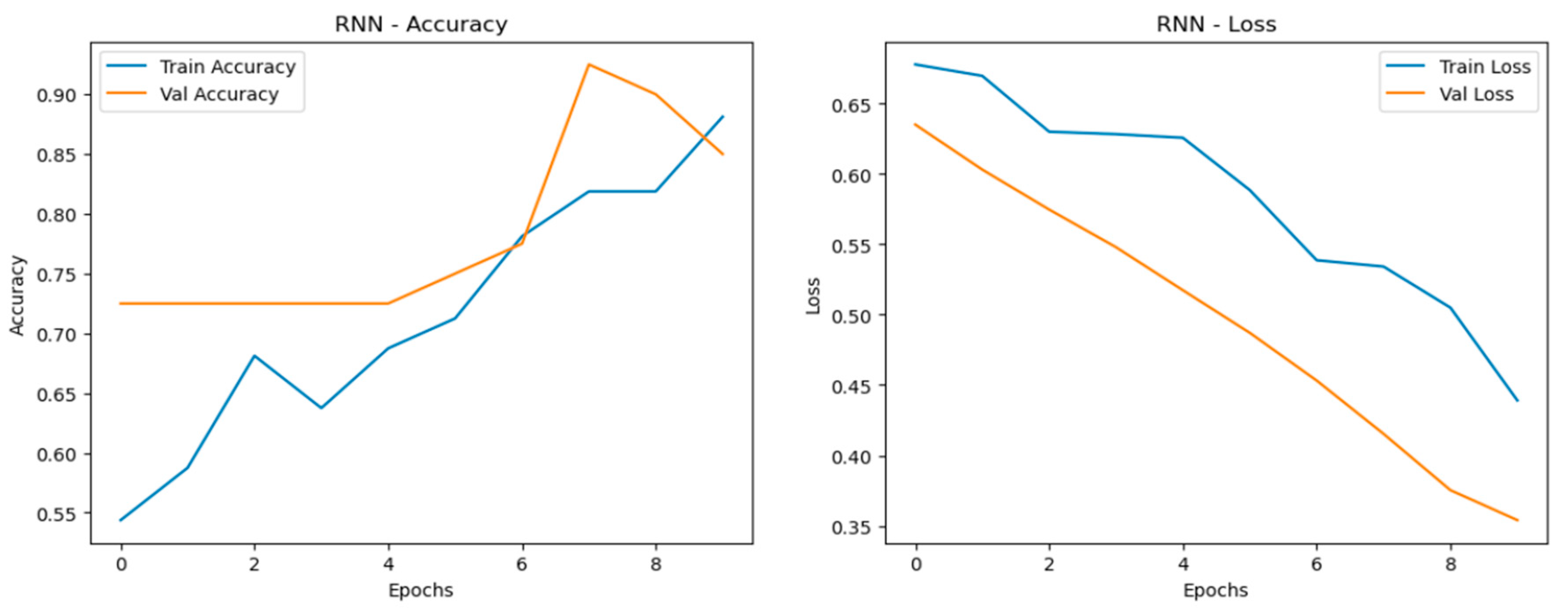
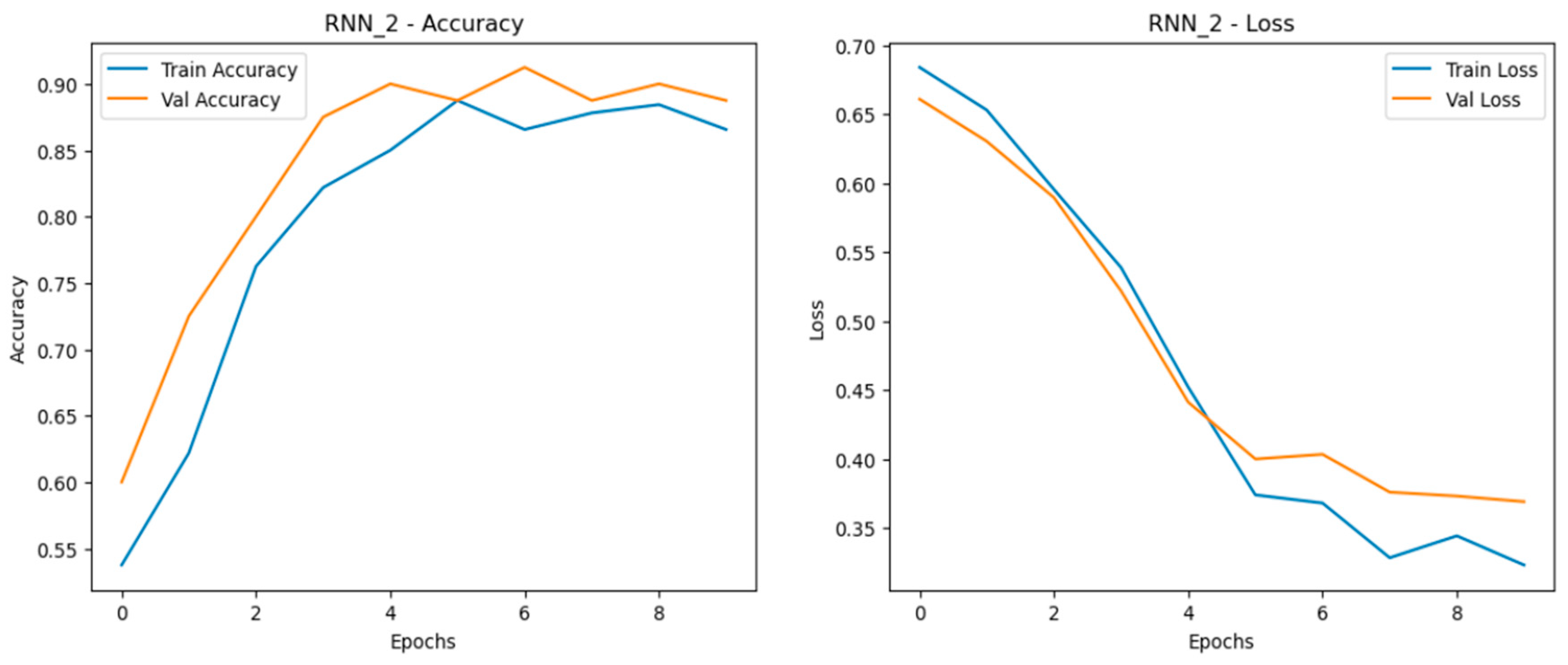
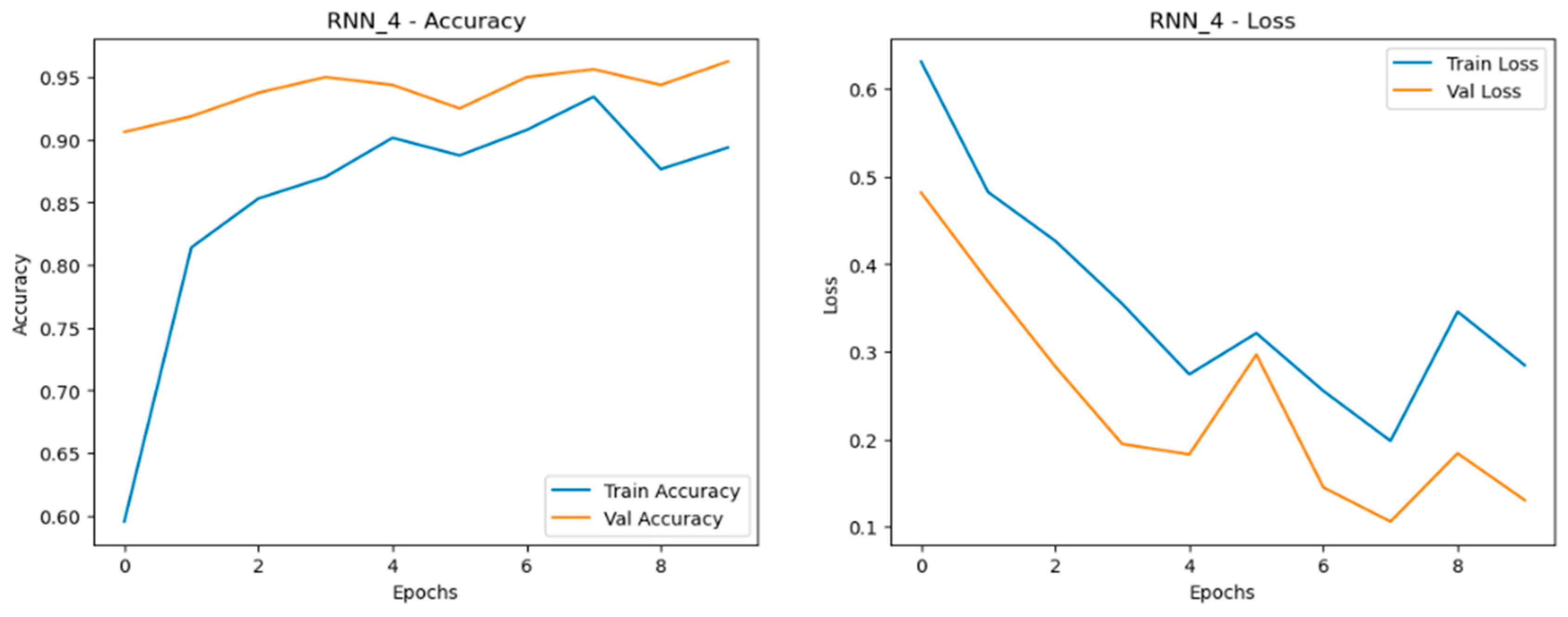
The Recurrent Neural Network (RNN) models displayed fluctuating performance as data was scaled, with accuracy and generalization stability being less consistent compared to the MLP and CNN models. While the RNN models performed reasonably well, they showed more variation between training and validation accuracy curves, particularly as dataset size increased. This fluctuation suggests that RNNs struggle to maintain consistent learning across different data volumes. The loss curves for RNNs revealed greater volatility, indicating less stable learning, especially with larger datasets. Despite these challenges, the RNN models still managed to achieve decent alignment between training and validation curves, particularly in the quadrupled dataset (RNN_4), which was the best-performing set among the RNN models as shown in
Figure 21,
Figure 22 and
Figure 23. Although capable, RNNs were less reliable in scaling effectively compared to simpler architectures like MLP and CNN.
- 1.
Normal Dataset
Figure 21.
Training and validation metrics for RNN normal dataset.
Figure 21.
Training and validation metrics for RNN normal dataset.
- 2.
Doubled Dataset
Figure 22.
Training and validation metrics for RNN dataset doubled.
Figure 22.
Training and validation metrics for RNN dataset doubled.
- 3.
Quadrupled Dataset
Figure 23.
Training and validation metrics for RNN dataset quadrupled.
Figure 23.
Training and validation metrics for RNN dataset quadrupled.
4. LSTM (Long Short-Term Memory)
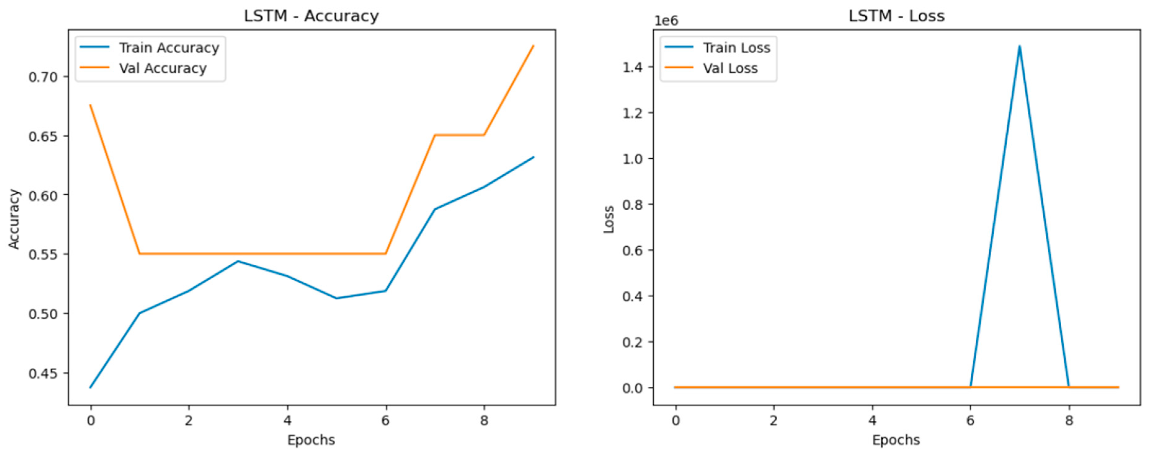
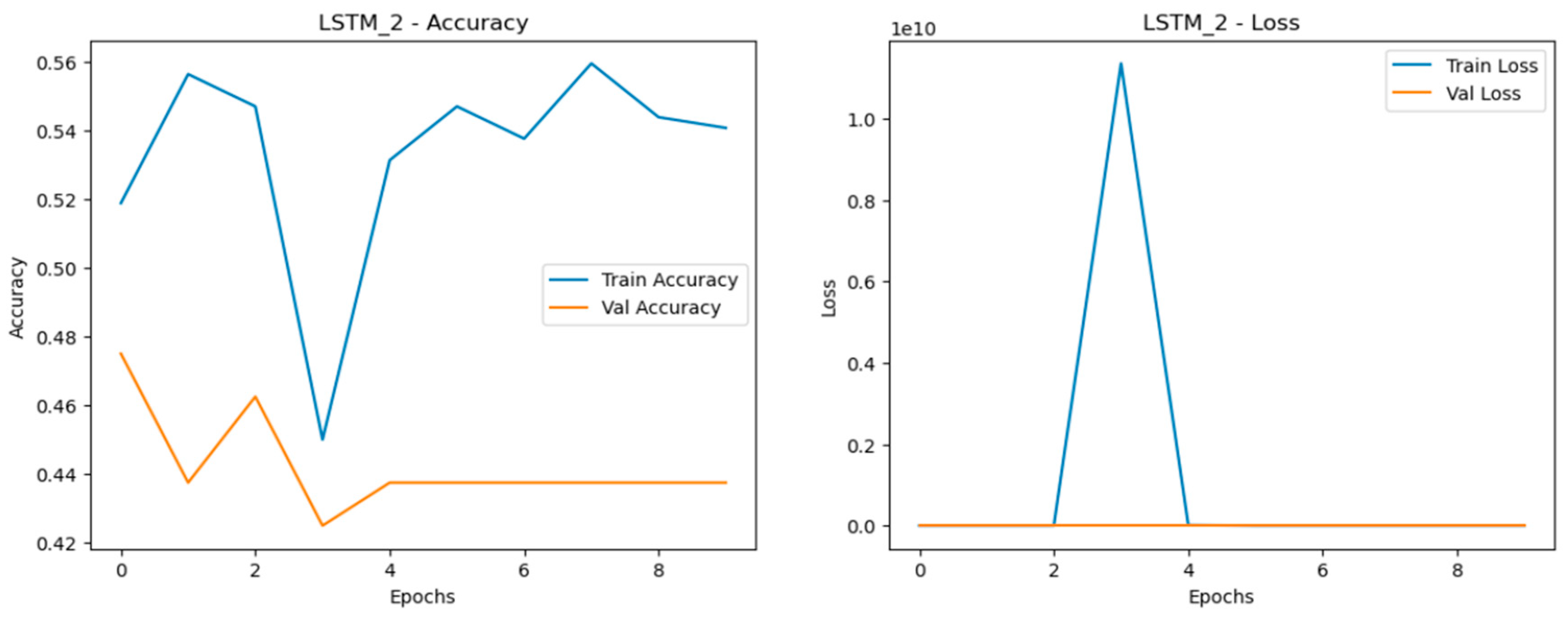
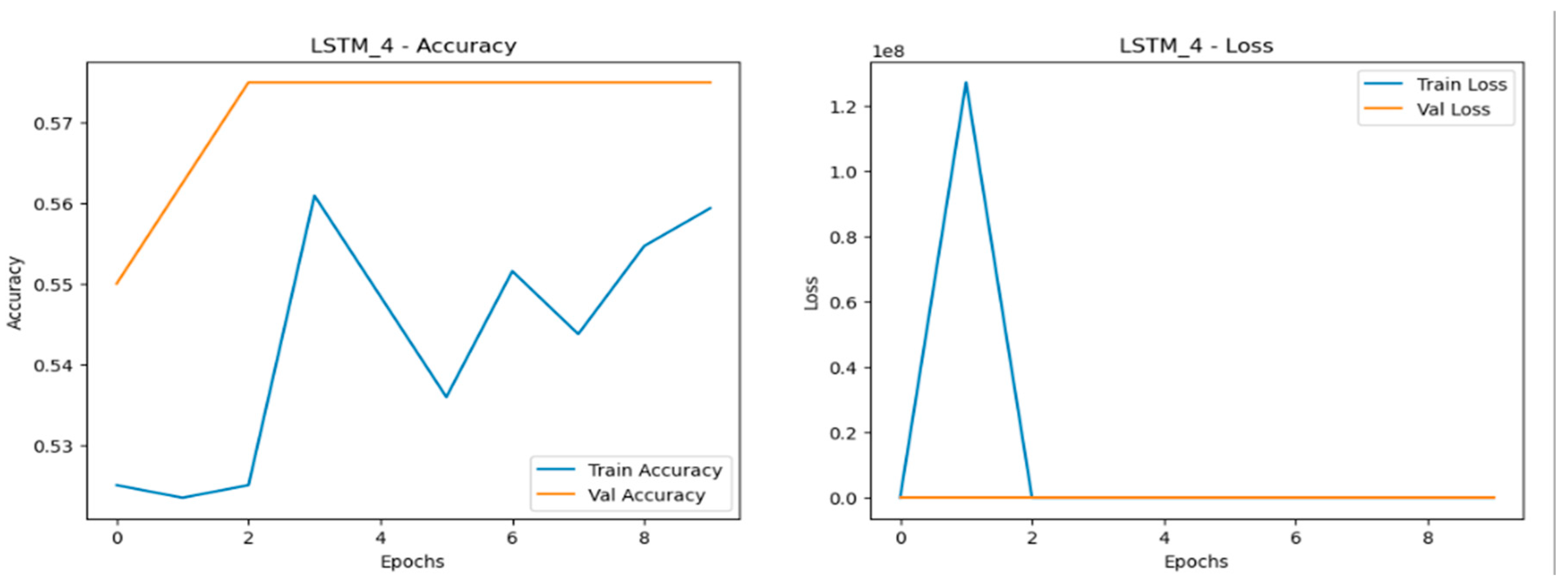
The Long Short-Term Memory (LSTM) models encountered the most difficulty when dealing with data scaling, with significant drops in accuracy, precision, recall, and F1-score as the dataset size increased as shown in
Figure 24,
Figure 25 and
Figure 26. The LSTM models showed notable fluctuations in accuracy across all datasets, struggling to maintain stable learning and generalization. This issue was particularly pronounced in larger datasets, where the models had trouble capturing patterns effectively. The loss curves for LSTM were highly erratic, featuring sharp spikes, especially in validation loss, signaling overfitting and poor generalization. The most problematic performance was observed in the quadrupled dataset (LSTM_3), where the model exhibited highly unstable behavior with substantial variation in both accuracy and loss, making it the weakest performer overall. This inconsistency indicates that LSTM models were the least reliable when scaling data in this experiment.
. Normal Dataset
Figure 24.
Training and validation metrics for LSTM normal dataset.
Figure 24.
Training and validation metrics for LSTM normal dataset.
Figure 25.
Training and validation metrics for LSTM dataset doubled.
Figure 25.
Training and validation metrics for LSTM dataset doubled.
- 3.
Quadrupled Dataset
Figure 26.
Training and validation metrics for LSTM dataset quadrupled.
Figure 26.
Training and validation metrics for LSTM dataset quadrupled.
The performance analysis across scaled datasets reveals that the Multilayer Perceptron (MLP) consistently outperformed other models, demonstrating near-perfect accuracy, stability, and generalization across all dataset sizes. The Convolutional Neural Network (CNN) also performed strongly, showing robust accuracy and effective learning with minimal overfitting even as data scaled. While the Recurrent Neural Network (RNN) achieved decent results, it exhibited more fluctuations in accuracy and stability, especially in larger datasets. The Long Short-Term Memory (LSTM) model, however, struggled the most, with significant drops in performance, erratic loss curves, and pronounced overfitting issues as the dataset size increased. Overall, the analysis highlights that simpler models like MLP and CNN were better suited for this specific problem, while LSTM struggled to handle the complexity introduced by larger datasets.
8. Conclusion and Future Recommendation
By systematically varying fault conditions, the experimental setup in this work aimed to replicate realistic operational scenarios that machinery might experience in the manufacturing machine. The results derived from both balanced and imbalanced conditions offer a robust foundation for condition monitoring and analysis. The controlled introduction of weights provides a comprehensive dataset for training and validating diagnostic models, which are essential for detecting and predicting faults.
According to the analysis and discussions in the previous section, the methods of DL Which includes MLP, CNN and RNN is not only adaptively extract the fault information, but also overcoming the disadvantages of many traditional methods. Although the proposed methods in this research have achieved some promising results in rotary machinery, there are still many challenges in the current researches in selecting right DL technique and the future directions of the research. There are some limitations in this study.
Hyperparameter Tuning: The algorithms were not fine-tuned through hyperparameter optimization, which may have limited their potential to achieve the highest possible accuracy.
Limited Data Volume: The dataset was relatively small, which constrained the model’s ability to generalize, particularly in predicting fault weights accurately.
Minimal Preprocessing: Data preprocessing was intentionally kept minimal, which, while simplifying the model pipeline, may have restricted the model’s ability to fully leverage the data’s informative features.
Limited Generalizability: The findings are based on data generated from the Spectra Quest Machinery Fault Simulator. Performance may vary when these models are applied to real-world scenarios with different machinery, operating conditions, or fault types.
The findings from this study contribute to the development of more accurate and reliable condition monitoring techniques, enhancing predictive maintenance strategies. This, in turn, can lead to extended operational life, reduced downtime, and improved overall efficiency of industrial machinery. In comparison to the algorithms between MLP, CNN, RNN and LSTM, CNN has given 95% of accuracy compared to the MLP of 90%. The RNN and LSTM is not giving promising result for the dataset which we have taken for the analysis. It doesn’t mean that RNN and LSTM will not give an accurate result in all cases. The lower performance of RNN and LSTM may be attributed to their sensitivity to noise or the specific temporal dynamics of the data not aligning well with these models’ strengths. CNN’s superior performance is primarily due to its ability to capture spatial patterns and localized features in the data, making it well-suited for tasks involving structured or spatially dependent information [
48]. However, MLP’s robust performance, despite its simpler architecture, demonstrates its adaptability and consistent learning across scaled datasets giving an accuracy of 100%. MLP’s fully connected structure allows it to utilize all input features equally without prioritizing spatial hierarchies, which can be an advantage when the task does not heavily rely on spatial dependencies. So, we can conclude that the DL is the future of maintenance engineering in which the fault diagnosis will be carried out with more accuracy in this modern industrial revolution.
Author Contributions
Conceptualization, K.V. and R.A .; Literature collection, K.V.,R.A.,M.K and S.RK.A.V; Formal analysis, R.A,K.V. and M.K. ; Funding acquisition, R.A., K.V. and KPR ; Investigation, R.A.,K.V and M.K ; Methodology, R.A., KPR, K.V.,M.K., and S.RK.A.V ; Validation, R.A. and K.V.; Writing—original draft, R.A.; Review and editing, R.A., M.K., KPR, K.V. and S.RK.A.V. All authors have read and agreed to the published version of the manuscript.
Funding
This work was performed as part of the research work titled” Deep learning based real time drill condition monitoring using acoustic emission sensor” funded by MOHERI, OMAN, grant number BFP/RGP/EI/22/433.
Institutional Review Board Statement
This study was conducted according to the guidelines of the National University of science and Technology, Oman.
Data Availability Statement
The original contributions presented in the study are included in the article/supplementary material, further inquiries can be directed to the corresponding author/s.
Conflicts of Interest
The authors declare no conflict of interest.
References
- Maamar Ali Saud Al Tobi, Ramachandran K p, Saleh Al-Araimi, Rene Pacturan, Amuthakkannan Rajakannu, and Geetha Achuthan. 2022. Machinery Fault Diagnosis using Continuous Wavelet Transform and Artificial Intelligence based classification. In Proceedings of the 2022 3rd International Conference on Robotics Systems and Vehicle Technology (RSVT ‘22). Association for Computing Machinery, New York, NY, USA, 51–59. [CrossRef]
- Amuthakkannan Rajakannu, Ramachndran, KP, Vijayalakshmi,K (2024). Application of Artificial Intelligence in Condition Monitoring for Oil and Gas Industries. Preprints 2024, 2024090752. [CrossRef]
- Amuthakkannan Rajakannu, Ramachndran, KP, Vijayalakshmi,K (2024),. Condition Monitoring of Drill Bit for Manufacturing Sector Using Wavelet Analysis and Artificial Neural Network (ANN). Preprints 2024, 2024060859. [CrossRef]
- Maamar Ali Saud AL Tobi , Ramachandran. KP. , Saleh AL-Araimi , Rene Pacturan, Amuthakannan Rajakannu , Chetha Achuthan (2022), Machinery Faults Diagnosis using Support Vector Machine (SVM) and Naïve Bayes classifiers, International Journal of Engineering Trends and Technology ,Volume 70 Issue 12, 26-34, December 2022. [CrossRef]
- Waleed Abdulkarem, Rajakannu Amuthakkannan, and Khalid F. Al-Raheem, (2014), Centrifugal Pump Impeller Crack Detection Using Vibration Analysis, 2nd International Conference on Research in Science, Engineering and Technology (ICRSET’2014), March 21-22, 2014 Dubai (UAE).
- Onur Surucu, Stephen Andrew Gadsden, John Yawney, Condition Monitoring using Machine Learning: A Review of Theory, Applications, and Recent Advances, Expert Systems with Applications, Volume 221,2023,119738,ISSN 0957-4174. [CrossRef]
- Serin, G., Sener, B., Ozbayoglu, A. M., & Unver, H. O. (2020). Review of tool condition monitoring in machining and opportunities for deep learning. International Journal of Advanced Manufacturing Technology, 109(3–4), 953–974. [CrossRef]
- Josef Koutsoupakis, Panagiotis Seventekidis, Dimitrios Giagopoulos,Machine learning based condition monitoring for gear transmission systems using data generated by optimal multibody dynamics models, Mechanical Systems and Signal Processing, Volume 190,2023,110130,ISSN 0888-3270.
- Zhang L, Liu Y, Zhou J, Luo M, Pu S, Yang X. An Imbalanced Fault Diagnosis Method Based on TFFO and CNN for Rotating Machinery. Sensors (Basel). 2022 Nov 12;22(22):8749. [CrossRef] [PubMed]
- Erkki Jantunen (2002), A summary of methods applied to tool condition monitoring in drilling, International Journal of Machine Tools & Manufacture 42 (2002) 997–1010. [CrossRef]
- Pushkar Dehspande, Vigneashwara Pandiyan, Bastain Meylan & Kilian Wasmer, (2021) Acoustic emission and machine learning based classification of wear generated using a pin-on-disc tribometer equipped with a digital holographic microscope, Wear 476, 203622. [CrossRef]
- Rui Zhao, Ruqiang Yan, Zhenghua Chen, Kezhi Mao, Peng Wang, Robert X. Gao,Deep learning and its applications to machine health monitoring,Mechanical Systems and Signal Processing,Volume 115,2019,Pages 213-237,ISSN 0888-3270. [CrossRef]
- Lang Dai,Tianyu Liu,Zhongyong Liu,Lisa Jackson,Paul Goodall,Changqing Shen,and Lei Mao ( 2020) An Improved Deep Learning Model for Online Tool Condition Monitoring Using Output Power Signals, Journal of Shock and Vibration, Hindawi , Volume 2020, Article ID 8843314, 12 pages, Available from. [CrossRef]
- Wang, Q.; Wang, H.; Hou, L.; Yi, S. (2021) Overview of Tool Wear Monitoring Methods Based on Convolutional Neural Network. Appl. Sci. 2021, 11, 12041. [CrossRef]
- Cerrada M., Sánchez R., Li C., Pacheco F., Cabrera D., Valente De Oliveira J., Vásquez R.E. A review on data-driven fault severity assessment in rolling bearings. Mech. Syst. Signal Process. 2018;99:169–196. [CrossRef]
- Janssens O., Slavkovikj V. Convolutional Neural Network Based Fault Detection for Rotating Machinery. J. Sound Vib. 2016;377:331–345. [CrossRef]
- Yao Y., Zhang S., Yang S., Gui G. Learning Attention Representation with a Multi-Scale CNN for Gear Fault Diagnosis under Different Working Conditions. Sensors. 2020;20:1233. [CrossRef]
- Zhang W., Li C., Peng G., Chen Y., Zhang Z. A deep convolutional neural network with new training methods for bearing fault diagnosis under noisy environment and different working load. Mech. Syst. Signal Process. 2018;100:439–453. [CrossRef]
- Manar Abdelmaksoud, Marwan Torki, Mohamed El-Habrouk, Medhat Elgeneidy,Convolutional-neural-network-based multi-signals fault diagnosis of induction motor using single and multi-channels datasets, Alexandria Engineering Journal,Volume 73,2023,Pages 231-248,ISSN 1110-0168. [CrossRef]
- Marwala, T. (2012). Multi-Layer Perceptron for Condition Monitoring in a Mechanical System. In: Condition Monitoring Using Computational Intelligence Methods. Springer, London. [CrossRef]
- Dino Žanić and Alan Župan ( 2023), Monitoring Transformer Condition with MLP Machine Learning Model, VOL. 72 NO. 2 (2023): JOURNAL OF ENERGY - ENERGIJA (02/2023).
- V. -Q. Nguyen, M. -H. Vu, V. -T. Pham and T. -T. Tran, “A Deep Learning Approach based on MLP-mixer Models for Bearing Fault Diagnosis,” 2023 International Conference on System Science and Engineering (ICSSE), Ho Chi Minh, Vietnam, 2023, pp. 16-21. [CrossRef]
- Tarek, K., Abdelaziz, L., Zoubir, C., Kais, K., and Karim, N. (2021). Optimized multi layer perceptron artificial neural network based fault diagnosis of induction motor using vibration signals. Diagnostyka, 22(1), pp.65-74. [CrossRef]
- Neupane, D.; Kim, Y.; Seok, J.; Hong, J. CNN-Based Fault Detection for Smart Manufacturing . Appl. Sci. 2021, 11, 11732. [CrossRef]
- Lundgren, A., & Jung, D. (2022). Data-driven fault diagnosis analysis and open-setclassification of time-series data.Control Engineering Practice,121, Article 105006. [CrossRef]
- Li, G., Wu, J., Deng, C., Xu, X., & Shao, X. (2021). Deep reinforcement learning-based online domain adaptation method for fault diagnosis of rotating machinery.IEEE/ASME Transactions on Mechatronics. [CrossRef]
- Lei, Y., Karimi, H. R., Cen, L., Chen, X., & Xie, Y. (2021). Processes soft modeling basedon stacked autoencoders and wavelet extreme learning machine for aluminumplant-wide application.Control Engineering Practice,108, Article 104706. [CrossRef]
- Tian, J., Han, D., Li, M., & Shi, P. (2022). A multi-source information transferlearning method with subdomain adaptation for cross-domain fault diagnosis.Knowledge-Based Systems,243, Article 108466. [CrossRef]
- Yang, D., Karimi, H. R., & Gelman, L. (2022). A fuzzy fusion rotating machineryfault diagnosis framework based on the enhancement deep convolutional neuralnetworks.Sensors,22(2), 671. [CrossRef]
- Lei, Y., Karimi, H. R., & Chen, X. (2022). A novel self-supervised deep LSTM network for industrial temperature prediction in aluminum processes application.Neurocomputing,502, 177–185. [CrossRef]
- Zhou, F., Yang, S., Fujita, H., Chen, D., & Wen, C. (2020). Deep learning fault diagnosismethod based on global optimization GAN for unbalanced data.Knowledge-BasedSystems,187, Article 104837.12. [CrossRef]
- Wang, H.; Yang, T.; Han, Q.; Luo, Z. Approach to the quantitative diagnosis of rolling bearings.
- based on optimized VMD andLempel–Ziv complexity under varying conditions.Sensors2023,23, 4044.
- Chen, L.; Liu, X.; Zeng, C.; He, X.; Chen, F.; Zhu, B. Temperature prediction of seasonal frozen subgrades based on CEEMDAN-LSTM hybrid model.Sensors2022,22, 5742. [CrossRef]
- Eren L, Ince T, Kiranyaz S (2018) A Generic Intelligent Bearing Fault Diagnosis System Using Compact Adaptive 1DCNN Classifier. Journal of Signal Processing Systems. [CrossRef]
- Zhang, W.; Li, X.; Ding, Q. Deep residual learning-based fault diagnosis method for rotating machinery.ISA Trans.2019,95, 295–305. [CrossRef]
- Diwang Ruan, Jin Wang, Jianping Yan, Clemens Gühmann, CNN parameter design based on fault signal analysis and its application in bearing fault diagnosis,Advanced Engineering Informatics,Volume 55,2023,101877,ISSN 1474-0346. [CrossRef]
- Achyuth Kothuru, Sai Prasad Nooka, Rui Liu,Application of deep visualization in CNN-based tool condition monitoring for end milling,Procedia Manufacturing,Volume 34,2019,Pages 995-1004,ISSN 2351-9789. [CrossRef]
- Jia F., Lei Y., Lu N., Xing S. Deep normalized convolutional neural network for imbalanced fault classification of machinery and its understanding via visualization. Mech. Syst. Signal Process. 2018;110:349–367. [CrossRef]
- Serhat Şeker, Emine Ayaz, Erduinç Türkcan,Elman’s recurrent neural network applications to condition monitoring in nuclear power plant and rotating machinery,Engineering Applications of Artificial Intelligence,Volume 16, Issues 7–8,2003,Pages 647-656,ISSN 0952-976. [CrossRef]
- Chris Halliday,Iain Palmer,Nigel Pready, Mark Joyce,(2022), A Recurrent Neural Network Method for Condition Monitoring and Predictive Maintenance of Pressure Vessel Components, ASME 2022 Pressure Vessels & Piping Conference,July 17–22, 2022,Las Vegas, Nevada, USA.
- Swetha R Kumar, Jayaprasanth Devakumar,Recurrent neural network based sensor fault detection and isolation for nonlinear systems: Application in PWR,Progress in Nuclear Energy,Volume 163,2023,104836,ISSN 0149-1970. [CrossRef]
- Yahui Zhang, Taotao Zhou, Xufeng Huang, Longchao Cao, Qi Zhou,Fault diagnosis of rotating machinery based on recurrent neural networks,Measurement,Volume 171,2021,108774,ISSN 0263-2241. [CrossRef]
- Zhuang Ye, Jianbo Yu,Health condition monitoring of machines based on long short-term memory convolutional autoencoder,Applied Soft Computing,Volume 107,2021,107379,ISSN 1568-4946. [CrossRef]
- H. Zhao, S. Sun and B. Jin, “Sequential Fault Diagnosis Based on LSTM Neural Network,” in IEEE Access, vol. 6, pp. 12929-12939, 2018. [CrossRef]
- Afridi, Y.S.; Hasan, L.; Ullah, R.; Ahmad, Z.; Kim, J.-M. LSTM-Based Condition Monitoring and Fault Prognostics of Rolling Element Bearings Using Raw Vibrational Data. Machines 2023, 11, 531. [CrossRef]
- Xie, J.; Du, G.; Shen, C.; Chen, N.; Chen, L.; Zhu, Z. An end-to-end model based on improved adaptive deep belief network and its application to bearing fault diagnosis. IEEE Access 2018, 6, 63584–63596. [CrossRef]
- Qiu, S.; Cui, X.; Ping, Z.; Shan, N.; Li, Z.; Bao, X.; Xu, X. Deep Learning Techniques in Intelligent Fault Diagnosis and Prognosis for Industrial Systems: A Review. Sensors 2023, 23, 1305. [CrossRef]
- SpectraQuest, Inc. (2020). User Operating Manual for Machinery Fault Simulator™. Richmond, VA: SpectraQuest, Inc.
- Ng, S., Tse, P. and Tsui, K. (2014). A One-Versus-All Class Binarization Strategy for Bearing Diagnostics of Concurrent Defects. Sensors, [online] 14(1), pp.1295–1321. [CrossRef]
- Nossier, S. A., Wall, J., Moniri, M., Glackin, C., & Cannings, N. (2020). A Comparative Study of Time and Frequency Domain Approaches to Deep Learning based Speech Enhancement. Journal of Signal Processing, 45(3), pp. 123-135. [Online]. Available at: http://vigir.missouri.edu/~gdesouza/Research/Conference_CDs/IEEE_WCCI_2020/IJCNN/Papers/N-21378.pdf.
- Yi, K., Zhang, Q., Fan, W., Wang, S., Wang, P., He, H., Lian, D., An, N., Cao, L., & Niu, Z. (2021). Frequency-domain MLPs are More Effective Learners in Time Series Forecasting. International Journal of Forecasting, 37(2), pp. 456-467. [Online]. Available at: https://proceedings.nips.cc/paper_files/paper/2023/file/f1d16af76939f476b5f040fd1398c0a3-Paper-Conference.pdf.
- Mali, A., Ororbia, A. G., Kifer, D., & Giles, C. L. (2023). Neural JPEG: End-to-End Image Compression Leveraging a Standard JPEG Encoder-Decoder. arXiv preprint. [Online]. Available at: https://arxiv.org/pdf/2201.11795.
- Hertel, L., Phan, H., & Mertins, A. (2022). Comparing Time and Frequency Domain for Audio Event Recognition Using Deep Learning. IEEE Transactions on Audio, Speech, and Language Processing, 30(1), pp. 789-798. [Online]. Available at: https://ieeexplore.ieee.org/document/7727635/authors#authors.
- Yan, Y.D., 2021. Fault Diagnosis and Prognosis Techniques for Complex Engineering Systems. Springer, Berlin.
- Yahui Zhang, Taotao Zhou, Xufeng Huang, Longchao Cao, Qi Zhou,Fault diagnosis of rotating machinery based on recurrent neural networks, Measurement, Volume 171,2021,108774,ISSN 0263-2241. [CrossRef]
- O’Shea, K., & Nash, R. (2015). An Introduction to Convolutional Neural Networks. arXiv preprint arXiv:1511.08458. [Online]. Available at: https://arxiv.org/pdf/1511.08458.
- LeCun, Y., Bengio, Y., and Hinton, G., 2015. Deep learning. Nature, 521(7553), pp.436-444.[Online]. Available at: https://www.nature.com/articles/nature14539.
- Zhong, Chaochun & Jiang, Yang & Wang, Limin & Chen, Jiayan & Zhou, Juan & Hong, Tao & Zheng, Fan. (2023). Improved MLP Energy Meter Fault Diagnosis Method Based on DBN. Electronics. 12. 932. [CrossRef]
- Hornik, K., Stinchcombe, M. and White, H., 1989. Multilayer feedforward networks are universal approximators. Neural networks, 2(5), pp.359-366.[Online]. Available at: https://www.sciencedirect.com/science/article/abs/pii/0893608089900208. [CrossRef]
- Krizhevsky, A., Sutskever, I. and Hinton, G.E., 2012. ImageNet classification with deep convolutional neural networks. Advances in neural information processing systems, 25, pp.1097-1105.[online]. Available at: https://papers.nips.cc/paper_files/paper/2012/hash/c399862d3b9d6b76c8436e924a68c45b-Abstract.html.
- He, K., Zhang, X., Ren, S. and Sun, J., 2016. Deep residual learning for image recognition. In: Proceedings of the IEEE Conference on Computer Vision and Pattern Recognition. Las Vegas, NV, 27-30 June 2016. IEEE, pp.770-778. [Online]. Available at: https://ieeexplore.ieee.org/document/7780459.
- Goodfellow, I., Bengio, Y. and Courville, A., 2016. Deep Learning. Cambridge, MA: MIT Press. [Online]. Available at: https://www.deeplearningbook.org/.
- He, K., Zhang, X., Ren, S. and Sun, J., 2015. Delving deep into rectifiers: Surpassing human-level performance on ImageNet classification. In: Proceedings of the IEEE International Conference on Computer Vision. Santiago, Chile, 7-13 December 2015. IEEE, pp.1026-1034. [Online]. Available at: https://ieeexplore.ieee.org/document/7410480.
- John McGonagle, Christopher Williams, and Jimin Khim. Recurrent Neural Network. url: https://brilliant.org/wiki/recurrentneural-network/ (Accessed on 13 Sep 2024).
- Hochreiter, S. and Schmidhuber, J., 1997. Long short-term memory. Neural computation, 9(8), pp.1735-1780.[Online]. Available at: https://www.bioinf.jku.at/publications/older/2604.pdf.
- Divyanshu Thakur, (2018), LSTM and its equations, Technical Article, Median. Available at: https://medium.com/@divyanshu132/lstm-and-its-equations-5ee9246d04af (Accessedd on 13 Sep 2024).
- Graves, A., 2012. Supervised sequence labelling with recurrent neural networks. Springer Science & Business Media.[Online]. Available at: https://www.cs.toronto.edu/~graves/preprint.pdf.
|
Disclaimer/Publisher’s Note: The statements, opinions and data contained in all publications are solely those of the individual author(s) and contributor(s) and not of MDPI and/or the editor(s). MDPI and/or the editor(s) disclaim responsibility for any injury to people or property resulting from any ideas, methods, instructions or products referred to in the content. |
© 2024 by the authors. Licensee MDPI, Basel, Switzerland. This article is an open access article distributed under the terms and conditions of the Creative Commons Attribution (CC BY) license (https://creativecommons.org/licenses/by/4.0/).

