Preprint
Article

Improvement of Electric Fish Optimization Algorithm for Standstill Label Combined with Levy Flight Strategy

Altmetrics

Downloads

62

Views

31

Comments

0

A peer-reviewed article of this preprint also exists.

This version is not peer-reviewed

Submitted:

14 September 2024

Posted:

16 September 2024

You are already at the latest version

Alerts
Abstract
The Electric Fish Optimization (EFO) Algorithm is inspired by the predation behavior and communication of weak electric fish. It is a novel meta-heuristic algorithm that attracts researchers because it has few tunable parameters,high robustness,and strong global search capabilities. Nevertheless, when operating in complex environments, the EFO algorithm encounters several challenges including premature convergence, susceptibility to local optimum, and issues related to passive electric field localization stagnation. To address these challenges, this study introduces an Adaptive Electric Fish Optimization Algorithm Based on Standstill Label and Level Flight (SLLF-EFO). This hybrid approach incorporates the Golden Sine Algorithm and Good Point Set Theory to augment the EFO algorithm’s capabilities, employs a variable step size Levy flight strategy to efficiently address passive electric field localization stagnation problems, and utilizes a standstill label strategy to mitigate the algorithm’s tendency to fall into local optimum during the iterative process. By leveraging multiple solutions to optimize the EFO algorithm, this framework enhances its adaptability in complex environments. Experimental results from benchmark functions reveal that the proposed SLLF-EFO algorithm exhibits improved performance in complex settings, demonstrating enhanced search speed and optimization accuracy This comprehensive optimization not only enhances the robustness and reliability of the EFO algorithm but also provides valuable insights for its future applications.
Keywords: 
Subject: Computer Science and Mathematics  -   Data Structures, Algorithms and Complexity

1. Introduction

In the mid-20th century, the establishment of bionics led scientists to seek new inspiration from living organisms. Consequently, many researchers developed bionic evolutionary algorithms, known as natural heuristic algorithms, based on the biological evolution mechanisms found in nature, to address complex real-life problems. Meta-heuristic algorithms, a broad category of heuristic algorithms, are particularly noteworthy as they do not depend on specific problem conditions and are applicable to a wide range of scenarios. Notable examples of meta-heuristic algorithms include Particle Swarm Optimization (PSO) and Genetic Algorithm (GA). Research on the optimization of meta-heuristic algorithms has consistently remained a prominent and dynamic area within the field. By optimizing meta-heuristic algorithms, significant improvements in algorithm performance can be achieved, particularly in tackling complex problems such as function combination optimization and function solving. This optimization is essential in meeting diverse application requirements [1].
The Electric Fish Optimization (EFO) algorithm, a novel swarm intelligence optimization algorithm within the metaheuristic framework, was introduced by Yilmaz and Sen in 2020. This algorithm draws inspiration from the foraging behavior and communication patterns of weak electric fish. These fish, which inhabit muddy waters with poor visibility, face challenges in perceiving their surroundings due to limited visual capabilities, particularly in low-light conditions. Consequently, they have developed a unique skill known as electrical localization, which enables them to sense and navigate their environment effectively [2].
The Electric Fish Optimization (EFO) algorithm, known for its characteristics of fewer tunable parameters, strong robustness, and excellent global search ability, has garnered significant attention from researchers. Deepa and Madhavan developed the HREFSO algorithm by integrating the EFO algorithm with Rat Swarm Optimization (RSO) to optimize the selection threshold of skin lesion segmentation models [3]. Ibrahim et al. demonstrated the efficacy of the EFO algorithm in feature selection, particularly in handling complex optimization problems [4]. Kumar and Karri innovatively combined the EFO algorithm with Earthworm Optimization to reduce latency in cloud computing environments [5]. Notably, Rao and Madhu introduced a hybrid algorithm that merges the EFO algorithm with the Dragonfly Algorithm, enhancing the efficiency of large-scale MIMO systems [6]. Similarly, R. Anirudh Reddy and N. Venkatram devised a hybrid algorithm by integrating Horse Swarm Optimization (HOA) into the EFO algorithm for optimal path selection in network routing [7]. Moreover, Viswanadham and Jayavel proposed a novel approach using a hybrid EFO algorithm and Harris Eagle Optimization for data protection in supply chain networks [8]. Additionally, the EFO algorithm finds applications in diverse fields such as the classification of artificial neural networks [9], economic load scheduling [10], and Connected and Autonomous Vehicle (CAV) technology [11].
In order to improve the efficiency of the Electric Fish Optimization (EFO) algorithm, this paper presents an adaptive Electric Fish Optimization algorithm based on standstill label and Levy flight (SLLF-EFO) to enhance the adaptability of the EFO to intricate environments. The proposed algorithm integrates strategies such as Levy flight, standstill label, and adaptive global range. These strategies effectively address the challenges faced by the algorithm and aim to improve its efficiency in various aspects, ultimately enabling it to find optima more effectively. The main contributions are as follows:
(1) This paper optimizes the EFO in complex environments by utilizing optimization schemes, including the theory of good point sets, distance thresholds, and the golden sine operator. These methods enhance the algorithm’s convergence speed within systematic optimization.
(2) Much of the existing research on meta-heuristic algorithm optimization focuses on avoiding local optima, without considering how to enable the algorithm to escape local optima once trapped. In addition to the systematic optimization strategies mentioned above, the SLLF-EFO algorithm proposed in this paper innovatively adopts a standstill label strategy to optimize the iterative process after getting stuck in a local optimum. This strategy allows the algorithm individuals to actively escape after identifying themselves as trapped in a local optimum, thereby indirectly improving the algorithm’s overall global search ability.
(3) During multiple experimental studies on the EFO, it was found that due to the randomness of the EFO algorithm’s values, there is a small probability that all the electric fish in the algorithm will be in passive electric field localization mode. Passive electric field localization requires the participation of individuals who use active electric field localization, but there are no individuals in the population with active electric field localization at this time, which will cause the algorithm to suddenly interrupt or stop running, a phenomenon referred to as passive electric field localization stagnation in this paper. Although the probability of this situation occurring is extremely small, this paper introduces a variable step size Levy flight strategy to address it, which not only improves the global search ability of the algorithm but also resolves the passive electric field localization stagnation problem mentioned above.

2. Electric Fish Optimization Algorithm and Its Problems

2.1. Electric Fish Optimization Algorithm

The Electric Fish Optimization Algorithm (EFO) divides the population into active and passive electro-located electric fish based on the magnitude of the electric field frequency of the weak electric fish itself. The active electro-located electric fish can be used to search for food and avoid danger within a limited range through the electric signals generated by themselves, while the passive electro-located electric fish can be used for electro-location through receiving electric signals [2]. The design of EFO algorithm mainly consists of three parts: population initialization, active electrical positioning, and passive electrical positioning.
(1) Population initialization
In the EFO algorithm, the core parameters of electric fish individuals are their own position, frequency and amplitude of their electrical signals. The population initialization adopts a random initialization scheme, which randomly generates the coordinate values of N electric fish individuals in the D-dimensional space.
After initializing the position, the electric fish will set the frequency value of its electrical signal according to its own position. The frequency value f i t of the i-th individual in the algorithm at the t-th iteration will be determined by the individual’s fitness value, that is:
f i t = f m i n + f i t w o r s t t f i t i t f i t w o r s t t f i t b e s t t f m a x f m i n
In equation (1), f i t i t is the fitness value of the i-th individual at the t-th iteration; f i t w o r s t t and f i t b e s t t represents the worst and best fitness values of the electric fish population at the t-th iteration, respectively; f m i n and f m a x are the minimum and maximum values of frequency, respectively. In the algorithm, this frequency is mainly used for probability calculation, so f m a x = 1 and f m i n = 0 are set.
The amplitude value of an individual determines the movable range of active electric field localization for electric fish, and also determines the probability of being perceived by passive electric field localization electric fish. In the EFO algorithm, the amplitude value A i t of the i-th individual at the t-th iteration is determined by the amplitude value A i t 1 from the previous iteration and the frequency value f i t at this time. The calculation formula is as follows:
A i t = α A i t 1 + 1 α f i t
In equation (2), α is a constant within the interval [ 0 , 1 ] , which determines the weight of the previous amplitude and the current frequency. The initial amplitude value of the i-th individual is equal to its current frequency value f i t .
In the EFO algorithm, after each iteration, individuals with higher frequency values ( N A ) use active electric field localization (active mode), while individuals with lower frequency values ( N P ) will perform passive electric field localization (passive mode) N A + N P = N . Afterwards, each individual moves in parallel according to their own situation to find the global optimum.
(2) Active electric field localization
In the EFO algorithm, the range of active electric field localization is limited, so active electric field localization determines the local search ability of the EFO algorithm. The range of motion of the i-th individual in active mode is determined by its current amplitude value A i , and its calculation formula is shown in (3):
r i = x m a x j x m i n j A i
The distance between the i-th and k-th individuals is determined by the Cartesian distance formula:
d i k = x i x k = j = 1 D ( x i j x k j ) 2
Afterwards, if there are no other individuals within the search range of the active individual, then the active individual will perform Brownian motion within the active electric field range, as shown in equation (5). If there are other individuals present, the individual will randomly select one active individual for position update, as shown in equation (6).
x i j c a n d = x i j + φ x k j x i j
x i j c a n d = x i j + φ r i
In equations (5) and (6), k is a randomly selected individual from other individuals within the search range, φ is a uniformly distributed random number within the interval [ 1 , 1 ] , and x i j c a n d represents the candidate position for individual i.
(3) Passive electric field localization
Unlike active electric field localization, passive electric field localization does not depend on the number of other active mode individuals around individual i, and its movable range is much larger than the range of active electric field localization. Therefore, in the EFO algorithm, passive electric field localization determines the algorithm’s global search ability.
The probability that individual k ( k N A ) in active mode is perceived by individual i ( i N P ) in passive mode, p k , is related to the individual amplitude values of all active modes and the distance between individual i and individual k. It is calculated using the Roulette Wheel Selection, and the formula is as follows:
p k = A k / d i k j N A A j / d i j
According to the probability value obtained from equation (7), select K individuals from N A , determine their reference position x r j using equation (8), and generate a new position x i j n e w using equation (9).
x r j = k = 1 K A k x k j k = 1 K A k
x i j n e w = x i j + φ x r j x i j
In this logic, it is still possible for individuals with higher frequencies to perform passive electrical localization. When this situation occurs, the individual will completely lose their location information. To avoid this situation, the EFO algorithm considers using equation (10) to update the candidate position of individual i in the j-th dimensional search space. Among them, r a n d j ( 0 , 1 ) is a random number uniformly distributed in the ( 0 , 1 ) interval.
x i j c a n d = x i j n e w , r a n d j ( 0 , 1 ) > f i x i j , e l s e
The final step in passive electric field localization is to use equation (11) to modify the candidate position of individual i in the j-th dimensional search space, in order to increase the diversity of the population.
x i j c a n d = x m i n j + φ x m a x j x m i n j r a n d 1 0 , 1 r a n d 2 0 , 1
In the process of individual population localization, if the generated candidate position coordinates in a certain dimension exceed the specified global search range, the boundary coordinates of that dimension are considered as the candidate position coordinates to avoid going out of bounds.
After processing, the EFO algorithm will perform movement, and individuals will compare the fitness values of the candidate position with the current position. If the fitness of the candidate position is better than the current position, the individual will move to the candidate position, otherwise they will not move.
The basic process of EFO algorithm is shown in Figure 1. This figure illustrates the workflow of the EFO algorithm, including population initialization, active electric field localization, and passive electric field localization. It highlights how individuals in the population switch between active and passive modes based on their frequency values, guiding the optimization process. Based on the active/passive electric field localization logic of the EFO algorithm, it can be concluded that the active electric field localization of the EFO algorithm enables active mode individuals to approach other active mode individuals, while passive mode individuals rely on passive electric field localization to approach the areas where active mode individuals gather, reflecting the aggregation behavior of EFO algorithm individuals.

2.2. Problems Encountered by EFO

When facing high-dimensional complex environments where the number of dimensions of an individual or the number of extreme values in the search environment is gradually increased, the optimization performance of the EFO algorithm is significantly reduced. The main problems that arise due to these limitations are as follows:
(1) Premature convergence
The characteristic of many heuristic algorithms, including the EFO algorithm, is to choose a better position to move than the current one. In complex environments, the individual’s reference position may not be better than the current position. At this time, the individual will not move, resulting in multiple ineffective iterations and a significant decrease in algorithm efficiency, which is known as premature convergence [12,13,14].
(2) Easy plunges into local optimum
Trapping into local optimum is a common problem faced by most heuristic algorithms, and once trapped in local optimum, individuals will find it difficult to escape [15,16]. Due to the clustering trend of electric fish, the EFO algorithm is also susceptible to this problem, reducing its optimization ability.
(3) Passive electric field localization stagnation
According to equations (7) and (8), it can be inferred that, the passive electric field localization operation of the EFO algorithm needs to refer to the position of the active individual in the field. During the operation of the EFO algorithm, there may be a situation where the electrical signal frequency of all individuals is very low, and all individuals are in passive mode. In this case, if there are no active mode individuals on the field, it will be difficult for all passive individuals to move and the algorithm will come to a standstill. After testing, the probability of this situation occurring is very small, which is referred to as the passive electric field localization stagnation problem in this article.

3. The SLLF-EFO Algorithm Proposed in This Article

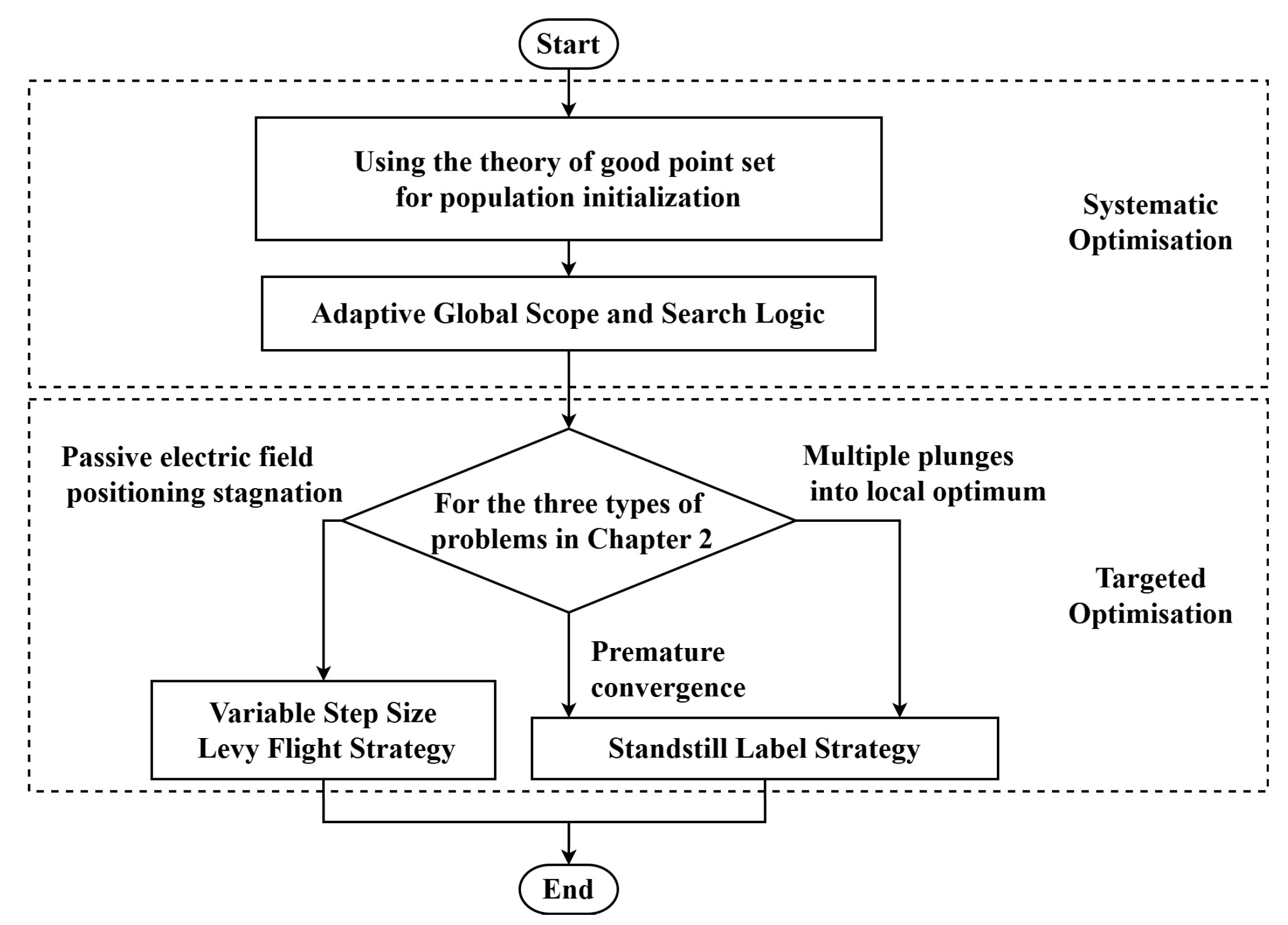
The Adaptive Electric Fish Optimization Algorithm Based on Standstill Label and Levy Flight (SLLF-EFO) proposed in this paper is an optimization scheme for the EFO algorithm, which incorporates standstill label and Levy flight strategies. This scheme includes both systematic and targeted optimizations for addressing the three aforementioned problems, thereby enabling the EFO algorithm to maintain high efficiency in diverse environments. The overall optimization strategy is illustrated in Figure 2. This figure presents the various strategies incorporated into the SLLF-EFO algorithm to enhance its performance. In terms of systematic optimization, the use of good point set theory for population initialization, adaptive global scope, individual selection optimization and the introduction of the golden sine operator were used to improve the speed of the EFO algorithm. In terms of targeted optimization, the variable step size Levy flight strategy and the standstill label strategy methods were used to solve the three problems mentioned in Section 2.2, which not only enabled the EFO algorithm to jump out of local optimum, but also improved its global search ability.

3.1. Population Initialisation

This article introduces a theory called good point set in the EFO algorithm for population initialization, rather than choosing traditional random schemes. The concept of the good point set was initially proposed by Italian economist Pareto, and further developed by mathematician Hua Luogeng on this basis [17]. Compared to random point set, good point set provide better coverage of the entire search space and are used to optimise various meta-heuristic algorithms [18,19].
Let G D be a unit cube in a D-dimensional Euclidean geometric space, if the position r G D , then for P n ( i ) = ( r 1 ( n ) · i , r 2 ( n ) · i , , r D ( n ) · i ) , 1 i n , its deviation φ ( n ) = C ( r , ε ) n 1 + ε , where C ( r , ε ) is a constant related only to r, ε , then it is called P n ( i ) to be the set of good points and r to be the good point.
In this paper, we take r i = 2 cos ( 2 π i p ) , 1 i D where p is the smallest prime number that satisfies p 3 2 D the smallest prime number.
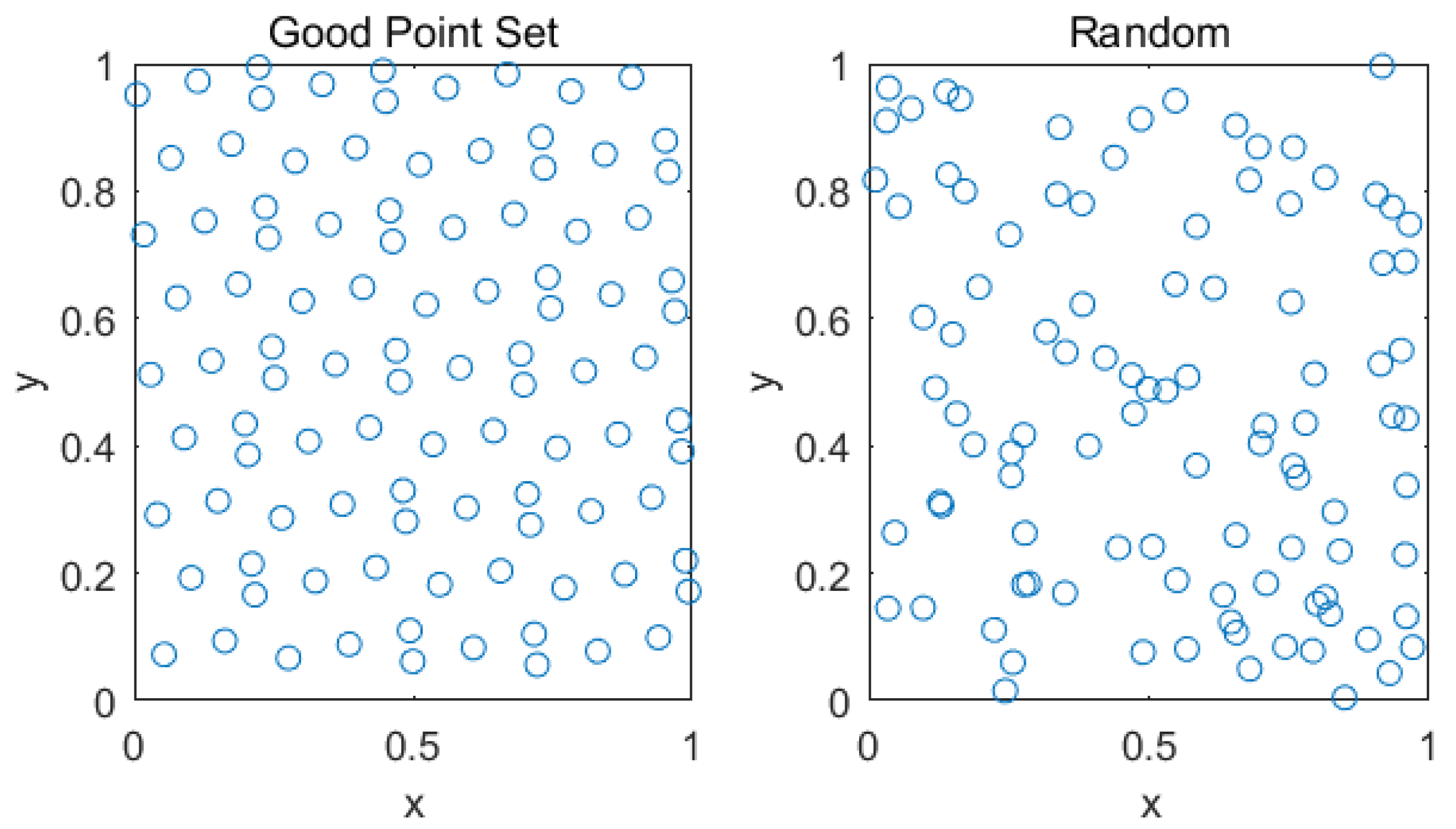
In order to evaluate the effectiveness of the best point set method, 100 initial population positions were created in the 2D plane using both the best point set and random placement methods. The results are shown in Figure 3. The left panel shows the initial population distribution using the good point set method, which is more uniform. The right panel shows the distribution using the random method. The results indicate that the initialization population distribution generated using the best point set method is more uniform, which can enhance the global search ability of the EFO algorithm to a certain extent.

3.2. Adaptive Global Scope and Search Logic

3.2.1. Adaptive Global Scope

To improve the convergence speed of the algorithm, consider reducing the global range during the iteration process. However, in the early iterations of the algorithm, more new areas need to be discovered by the population, and it is not advisable to narrow the global scope at this time, as it will hinder the search for the global optimal value. Therefore, this article proposes the Adaptive Global Scope method, which is a dynamic adjustment method for the search range of the algorithm. Based on the historical worst fitness value, it determines when to shrink the global range and improve the convergence speed of the algorithm. This article determines the time point to initiate contraction based on the historical worst fitness values obtained in the experiment, which improves the efficiency of the region search process. Based on experimental results, it has been observed that setting the opening condition to one-tenth of the historical worst fitness value yields better performance in typical scenarios. The specific process of updating the global upper bound U l i m j and lower bound L l i m j for the j-th dimension under this strategy is as follows:
L l i m j = L l i m j , a l l b s t > a l l w s t + 9 f i t b s t 10 m i n X j , e l s e
U l i m j = U l i m j , a l l b s t > a l l w s t + 9 f i t b s t 10 m a x X j , e l s e
In equations (12), (13), the X j refers to the j-th dimensional set of coordinates of all individuals, a l l b s t and a l l w s t refer to the global historical best fitness value and historical worst fitness value of this experiment, respectively. And f i t b s t refers to the global optimal solution fitness value in this environment.

3.2.2. Optimization of Individual Selection Strategy for Active Electric Field Localization

In the active electric field localization stage of the EFO algorithm, the active electric field localization individual detects other individuals and randomly selects one to move. This article considers modifying this selection logic to select the individual closest to oneself for movement. And this logic will lead to rapid population aggregation in the early stage of iteration, as well as difficulty in escaping from local optima, which is not conducive to the algorithm’s search. Therefore, it is considered to set up far and near thresholds, so that the active individuals do not use the nearest distance moving scheme in the above cases, and switch to the random selection scheme of the original EFO algorithm. Experimental tests show that the number of individual dimension dim to set the distance threshold is more effective, the far distance threshold d M a x L i m and near threshold d M i n L i m satisfy equation (14).
d M a x L i m = 10 12 × d i m d M i n L i m = 10 17 × d i m

3.2.3. Introduction of Golden Sine Operator

Golden Sine Algorithm (GSA) is an Optimization algorithm based on the sine function and the golden section coefficient [20]. The algorithm was originally proposed by Erkan Tanyildizi et al. in 2017, the design of the algorithm is inspired by the sine function in mathematics, and the use of the sine function for computational iterative Optimization search has the advantages of fast convergence speed, good robustness, easy to implement, and fewer parameters and operators to regulate, which is used in different fields of problem solving [21,22].
GSA introduces the golden ratio coefficient in the position update process, allowing GSA to fully search the region that produces excellent solutions in each iteration process, rather than the entire region, improving the algorithm’s optimization speed and possessing strong local search ability. The formula for updating individual positions in the golden sine algorithm is:
V i j t + 1 = V i j t | sin ( r 1 ) | + r 2 · sin ( r 1 ) | x 1 P i j t x 2 V i j t |
In equation (15), V i j t denotes the current position of individual i in the j-th dimension; P i j t denotes the optimal position of all individuals in the j-th dimension of the optimal position; V i j t + 1 represents the new position of individual i in the j-th dimension; r 1 [ 0 , 2 π ] and r 2 [ 0 , π ] determine the search step and search direction, respectively, and both of which obey a normal distribution; x 1 and x 2 are adjustable parameters used to control the search space, and they satisfy the following relationship:
x 1 = a · τ + b · 1 τ
x 2 = a · 1 τ + b · τ
In equations (16) and (17), the τ is the golden section coefficient 5 1 2 . In order to continuously narrow down the search scope, the values of a and b are also adjusted according to the location of the individual, and the initial values of a and b are respectively π and π .
In this paper, the golden sine operator is introduced in the last step of the passive electric field localization stage to randomly selects the position of one dimension of an individual for updating. The optimised position update formula is shown below.
x i j c a n d = x i j | sin ( r 1 ) | + r 2 · sin ( r 1 ) | a 1 x p j a 2 x i j | r a n d 1 0 , 1 r a n d 2 0 , 1
In equation (18), x p j refers to the current position of the best individual in the j-th dimension of the population. To simplify the iterative process and improve the computational efficiency, this paper sets the coefficient a 1 and a 2 to fixed values as follows:
a 1 = π · τ + π · 1 τ
a 2 = π · 1 τ + π · τ )

3.3. Variable Step Size Levy Flight Strategy

3.3.1. Levy Flight Strategy

In this article, we consider introducing Levy flight strategy to address problem (3) discussed in Section 2.2. Levy flight, named after French mathematician Paul Levy and first proposed by Benoit Mandelbrot in 1982, is a special type of stochastic flight characterized by a heavy-tailed probability distribution of step size [23]. It deviates from traditional random walk processes such as Brownian motion by giving individuals a higher likelihood of moving over long distances, leading to increased uncertainty. Due to its heavy tailed distribution, Levy flight can better simulate natural random moving and is widely used in various meta-heuristic algorithms to optimize performance [24,25,26].
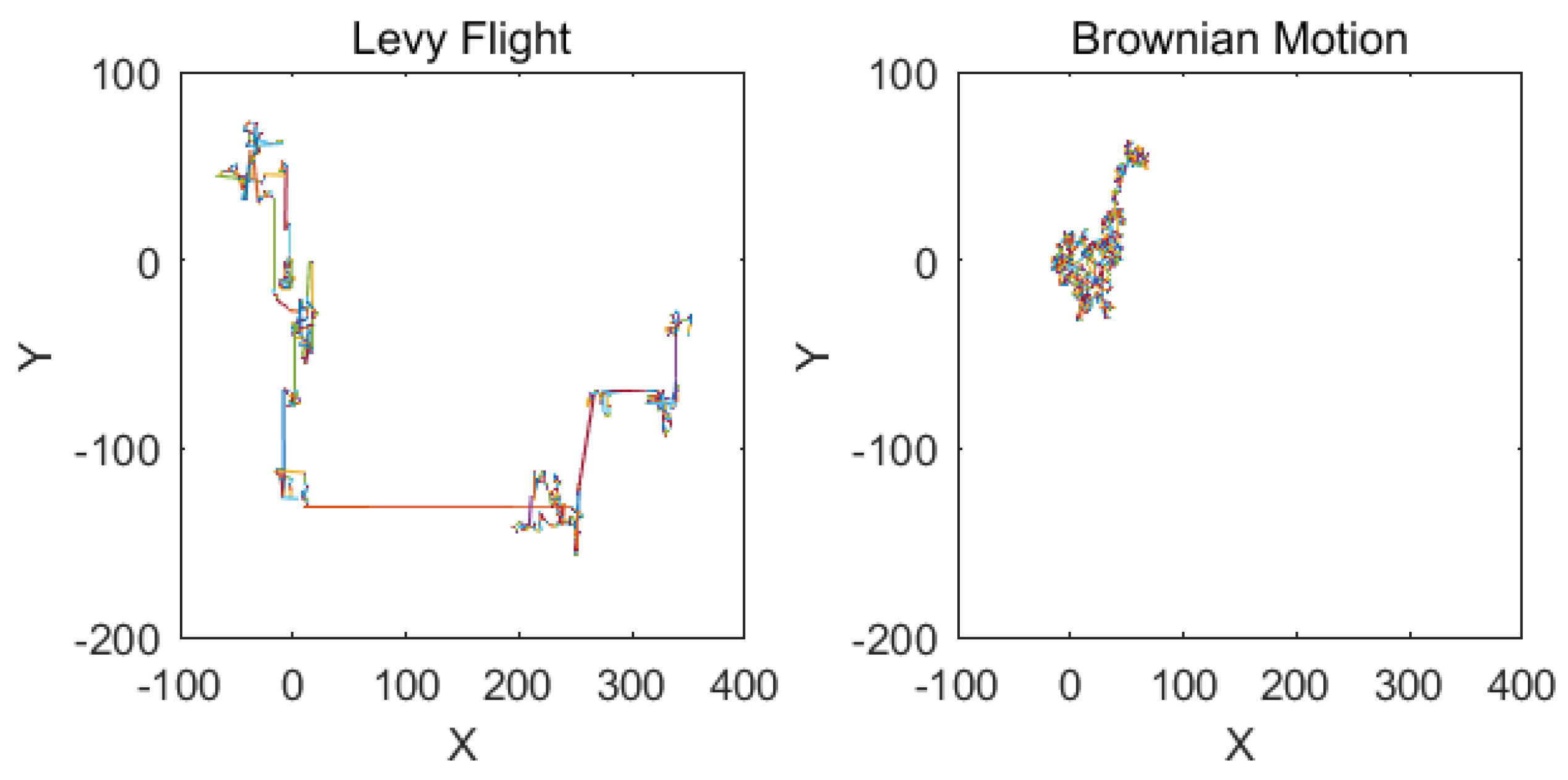
Figure 4 shows the results of 1000 Levy flights and 1000 Brownian motions performed by a single individual on a 2D plane. The left panel illustrates the trajectory of 1000 Levy flights, characterized by longer,sporadic jumps,enhancing the exploration capability. The right panel shows the trajectory of 1000 Brownian motions, characterized by shorter steps, which reflects the characteristic that Brownian motion can only search within a local range. From the figure, it can be seen that Levy flight relies on its high probability of long-distance flight to obtain a larger search range, which can improve the ability of individuals in the algorithm to discover new regions in applications.
Due to the extremely high complexity of the Levy flight, the Mantegna algorithm is commonly used to achieve a symmetric Levy stable distribution [27]. The probability density function of Levy flight step size under the Mantegna algorithm can be expressed as Equation (21):
L s s 1 β , 0 < β 2 s = μ v 1 β
In equation (21), s is the random step size, and β is the distribution parameter, μ and v are all intervals [ 0 , 1 ] random numbers obeying normal distribution within the interval.
By integrating Levy flight into the EFO algorithm, an individual will engage in Levy flight movement when passive electric field localization fails to detect any active mode individual. The introduction of Levy flight significantly broadens the activity range of the electric fish. This breakthrough not only breaks the stagnation phenomenon of the algorithm but also enhances the individual’s capacity to explore previously uncharted territories.

3.3.2. Variable Step Movement Logic

Experimental tests have shown that the aggregation behavior of EFO algorithm will cause most individuals to converge to the global optimum in the later stages of iteration. However, if Levy flight strategy is used again at this time, individuals may deviate from the global optimum due to long-distance movement. To alleviate this problem, this article considers adjusting the step size range of Levy flight at different times during the whole iteration process.
The Logistic model was proposed in 1837 by Verhulst, a German biologist, in his study of the laws of biological reproduction [28,29]. It is widely used to describe the process of saturation, known as the "S" process, and the Logistic model’s function curve, also referred to as the "S" curve, represents a gradual growth deceleration and stabilization phenomenon. The general function expression of the Logistic model is as follows:
f = α 1 + e β γ x
To introduce the Logistic model into the step size limitation strategy of Levy flight, it is necessary to integrate the fitness function of the EFO algorithm and determine the distance range of this Levy flight based on the current individual’s fitness value. The solution is to normalize the fitness values of individual i based on the best and worst historical fitness values of the population, in order to obtain the normalized fitness f i t i n o m , in order to import the Logistic model.
Adjust the logistic model function variables and substitute the normalized fitness values into them; When substituting, it is necessary to perform a scaling transformation on f i t i n o m to map it to the region range of the logistic model [-10,10]. However, when individuals approach local optima, their f i t i n o m are often small, which leads to a smaller step size for Levy flight and hinders individuals from escaping local optima. To address this issue, this article introduces a threshold. If the current normalized fitness of an individual is below this threshold, the step size range of Levy flight will be determined based on the number of iterations at that time. The experiment shows that the effect is better when the threshold is set to 10 4 , and the final step length formula is shown in equation (23), where i t e r c o u n t is the current iteration number.
s t e p i = 1 / 25 1 + e 10 20 f i t i n o m , f i t i n o m > 10 4 1 i t e r c o u n t , e l s e
In the end, the i-th individual performs a Levy flight with the logic of:
x i j n e w = x i j + s t e p i · s i g n r a n d 0.5 L e v y
In equation (24), s i g n r a n d 0.5 is the sign function, which is used to adjust the direction of the Levy flight, and it can enhance the randomness of the search and avoid falling into the local optimal solution. ⊗ is the point-to-point multiplication, Levy obeying equation (21).

3.4. Standstill Label Strategy

Issues (1) and (2) in Section 2.2 highlight a prevalent challenge known as stagnation, wherein individuals remain stationary for prolonged periods. Stagnation represents a common obstacle encountered by heuristic algorithms. While existing EFO optimization methods aim at preventing stagnation, strategies for addressing this state post-occurrence have not been thoroughly explored. To tackle the aforementioned challenges, a standstill label strategy is introduced in this paper as a novel approach.
The standstill label strategy originates from the living habits of ant colonies. When ant colonies explore, they leave pheromones on the paths they have already walked, guiding or reminding other individuals to follow up or change direction for search; Moreover, when individuals move to hazardous areas, warning pheromones are also released.When ant colony individuals recognize this pheromone, they will not approach or immediately move away from that location, which can greatly improve the search efficiency of the population [30].
SLLF-EFO uses a counter method to detect the stagnation of the best position individual. If the best position individual does not move after iteration, the counter is incremented by 1, otherwise it is cleared to zero. When the counter value reaches a certain value, the individual will be considered in a stagnant state. Due to the aggregation behavior of EFO, most individuals gather together during the counting process. Due to the close proximity of individuals, in order to improve the computational efficiency of the algorithm, the current behavioral state of the population can be determined by the position of the individual with the optimal fitness value at this time. When the best fitness individual is detected to be in a stagnant state, all individuals are forced to perform a variable step size Levy flight operation that is not limited by the global range and fitness function, and leave the pheromone at the best fitness individual position (stagnation point) before moving. After Levy flight, update the global scope again. This not only frees all individuals from local optima, but also avoids the problem of global optimal solutions not being within the global scope due to global scope contraction. When an individual moves to the stagnation point again, there is no need to perform another counting operation, but to directly perform a Levy flight operation and update the global range again, which causes the individual to immediately leave the position. This can effectively reduce the number of subsequent invalid iterations and improve the population’s ability to find the global optimum.

4. Experiments Based on Benchmark Functions

4.1. Test Functions and Comparison Algorithms

Due to the limitations of NP theory, it is difficult to prove the strict convergence of meta heuristic algorithms. In most cases, meta heuristic algorithms can only find approximate optimal values [31,32]. Therefore, many discussions on the convergence and optimization quality of metaheuristic algorithms are verified through experimental testing using standard test functions or a certain application scenario. The optimization performance of the algorithm is comprehensively obtained through comparative experiments in multi algorithm and multi function environments [33,34,35]. This article also adopts the method of using standard test functions to intuitively evaluate the optimization performance of the SLLF-EFO algorithm.
In order to visually evaluate the Optimization performance of the SLLF-EFO algorithm, this paper compares it with four algorithms in Python, including the original EFO algorithm and three classical meta-heuristic algorithms: the Particle Swarm Optimization (PSO) algorithm [36], Differential Evolution (DE) [37] and Genetic Algorithm (GA) algorithm [38]. The evaluation was performed using Python 3.11, with an AMD Radeon(TM) R5-5500U Graphics processor, Windows 11 operating system as the computational platform. Comparing with classical algorithms can fully demonstrate the optimization effect of SLLF-EFO algorithm.
12 CEC benchmark test functions, depicted in Table 1, have been chosen to assess the adaptability of the SLLF-EFO algorithm to intricate environments. The functions selected for this study can be referenced in [39] and [40]. Among them, F1 to F4 are high-dimensional single-peak functions, F5 to F7 are high-dimensional multi-peak functions, F8 and F9 are low-dimensional single-peak functions, and F10 to F12 are low-dimensional multi-peak functions.
The learning factor in the PSO algorithm used for the experiments c 1 , c 2 are set to 2, the maximum value of inertia weight ω is 0.9, and the minimum value is 0.4; in the DE algorithm, the scaling factor is set to 0.9 and the crossover factor CR is 0.6; The GA algorithm used has a crossover probability of 0.6 and a mutation probability of 0.05.
To ensure the fairness of the experiment, all algorithms use the same parameters, their population size is set to 30 individuals, and the upper limit of iterations for each algorithm is set to 2000 times. Moreover, since four algorithms are based on random search Optimization algorithms, there is a certain degree of chance in the results of a single experiment. In order to avoid this situation and further reflect the robustness of the algorithms, each algorithm is run independently for 100 times on each benchmark function, and the minimum number of iterations (Min-Iter), the maximum number of iterations (Max-Iter), the average number of iterations (Mean-Iter), and the number of times exceeding the limit of the iteration (Over-Num) are taken as four indicators of the convergence speed of the algorithms. To reflect the convergence speed of the algorithm, the average value (Mean) and the standard deviation (Std) of the 100 experimental results are taken as the indexes for evaluating the search accuracy of them.

4.2. Speed Comparison with Other Algorithms

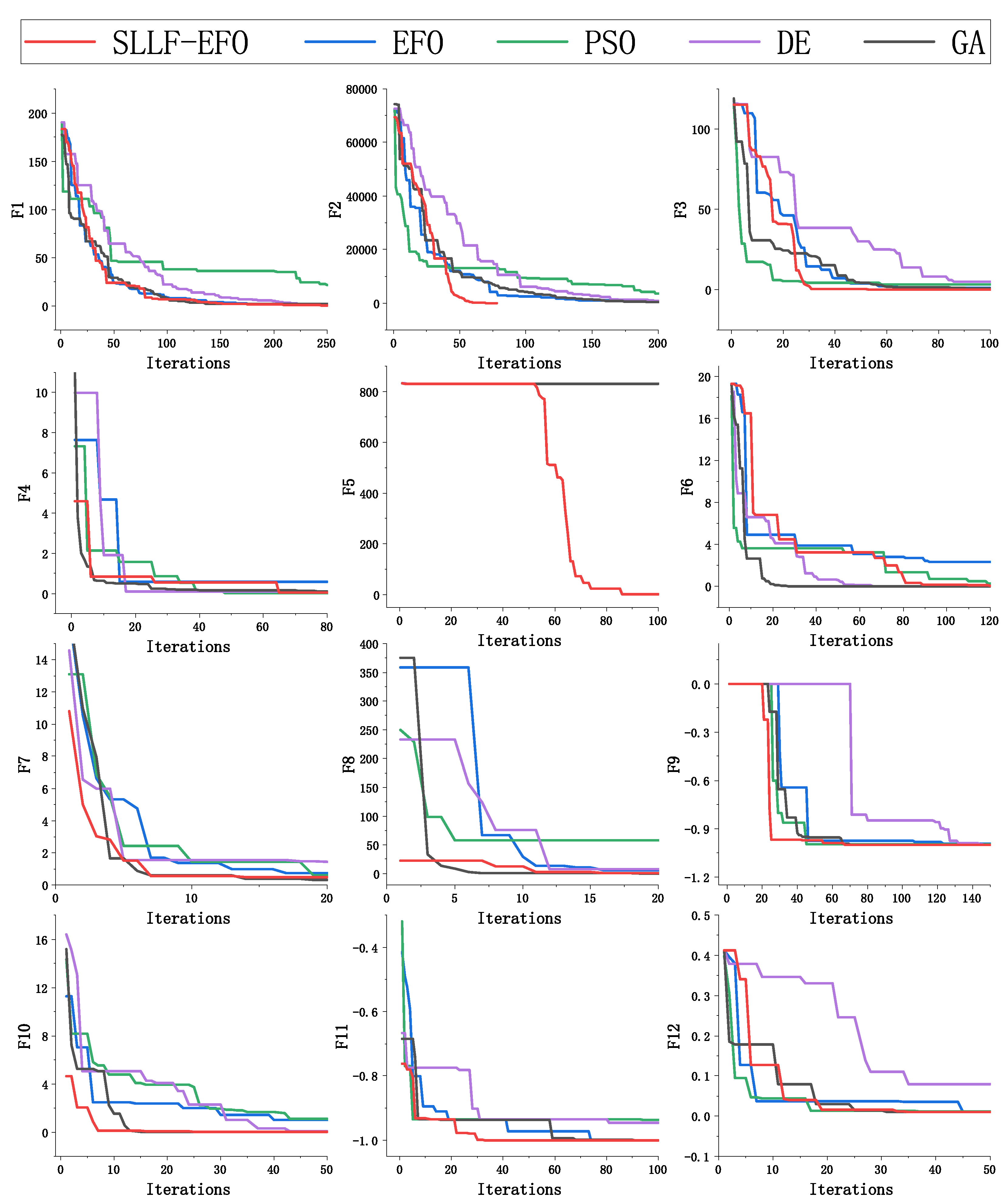
The speed index results of five algorithms conducting 100 experiments under different test functions are shown in Table 2. "Exceed" in this table indicates that the required number of iterations for the 100 experimental algorithms in this environment is greater than 2000. In addition to the three speed indicators, the last column in the table calculates the ratio of the average iteration times of the EFO and the SLLF-EFO in all function environments that can successfully converge, which is the speed improvement factor (SIF) of the SLLF-EFO. And to visually demonstrate the convergence process of the algorithm, select the parts of the iterative process with obvious convergence and draw an image as shown in Figure 5. These curves show the performance of SLLF-EFO, EFO, PSO, DE, and GA algorithms across 12 different benchmark functions. The X-axis represents the number of iterations,while the Y-axis represents the fitness value. The curves highlight the convergence speed of each algorithm, demonstrating the improved performance of the SLLF-EEO algorithm.
Based on Table 2 and Figure 5, the SLLF-EFO requires fewer iterations for optimization across 12 different test function environments compared to EFO. This suggests that the convergence speed of SLLF-EFO consistently outpaces that of EFO. Analysis of the GA data in the table reveals that the selected function tends to cause premature convergence and lead to the algorithm getting trapped in a local optimum. In contrast, SLLF-EFO demonstrates the ability to achieve convergence within 2000 iterations across the majority of environments. This underscores the effectiveness of the improved algorithm in addressing the issue of stagnation encountered in the original algorithm.
Table 2 shows that the number of iterations of SLLF-EFO in the environment of 12 different test functions is less than that of EFO. This indicates that the convergence speed of SLLF-EFO is stable and faster than that of EFO. Observing the data of the GA algorithm in the table, it can be seen that the selected function easily leads to premature convergence and stagnation in local optima of the algorithm. Observing the “Over-Num” metric, SLLF-EFO can converge within 2000 iterations in most environments, indicating that the improved algorithm effectively solves the problem of algorithm stagnation.
Observing the convergence curves of various algorithms in the early stage of iteration in Figure 5, it can be seen that under the F4, F7, F8, F10 and F11 functions, the initial fitness value of the SLLF-EFO is significantly better than the other four algorithms, which reduces the search difficulty of subsequent algorithms and fully verifies the optimization improvement of the good point set theory on population initialization.
In the F5 function environment depicted in Figure 5, all four algorithms, except for the SLLF-EFO, initially converged to local optima. Consequently, they remained stuck in these suboptimal solutions throughout the subsequent iterations, leading to premature convergence as illustrated by a horizontal straight line in the figure. In contrast, the SLLF-EFO incorporates a standstill label strategy. This strategy involves monitoring the algorithm’s progress using a counter mechanism. Specifically, after detecting that it has reached a local optimum following 50 consecutive iterations, the algorithm activates a standstill label strategy. This strategy facilitates the escape from local optimum and enabling individuals to explore the global search space. As evidenced by the convergence curve of F5, the SLLF-EFO algorithm exhibits a phase of horizontal convergence, followed by a resurgence in global search activity triggered by the standstill label strategy. This observation underscores the enhanced efficiency of the algorithm in seeking the global optimum through the implementation of the standstill label strategy.
Observing the optimization speed results of the SLLF-EFO and the other three meta-heuristic algorithms, it can be seen that the convergence speed of the SLLF-EFO is among the top in the five low dimensional environments of F8-F12, and in these low dimensional environments, the SLLF-EFO has the ability to find the global optimum. Except for the second place under the F9 function, all other environments only require the least number of iterations. In the high-dimensional complex environment of F1-F7, SLLF-EFO also maintains a high Optimization efficiency, and the most obvious improvement is in the F2 function, in the F2 function environment, SLLF-EFO is ahead of the other four algorithms with a great advantage of finding the optimal value in an average of 112 iterations, observing that Figure 5, it can be seen that SLLF-EFO has the top convergence speed in most environments.
Under the conditions that SLLF-EFO can find the globally optimum, observing the speed improvement multiple index, the algorithm in this paper requires fewer iterations than the EFO algorithm. This indicates that the improved SLLF-EFO algorithm has a high convergence speed in low dimensional environments.

4.3. Accuracy Comparison with Other Algorithms

In addition to the study of algorithm search speed, the study of algorithm optimization quality is also very important. Under many functions or application conditions, meta-heuristic algorithms such as EFO algorithm can only find approximate optimal values. Therefore, whether the algorithm can find an approximate value closer to the theoretical optimal value (i.e., accuracy) is particularly important. This article takes the average (Mean) and standard deviation (Std) of 100 experimental test results as indicators to evaluate the search quality of the SLLF-EFO algorithm.
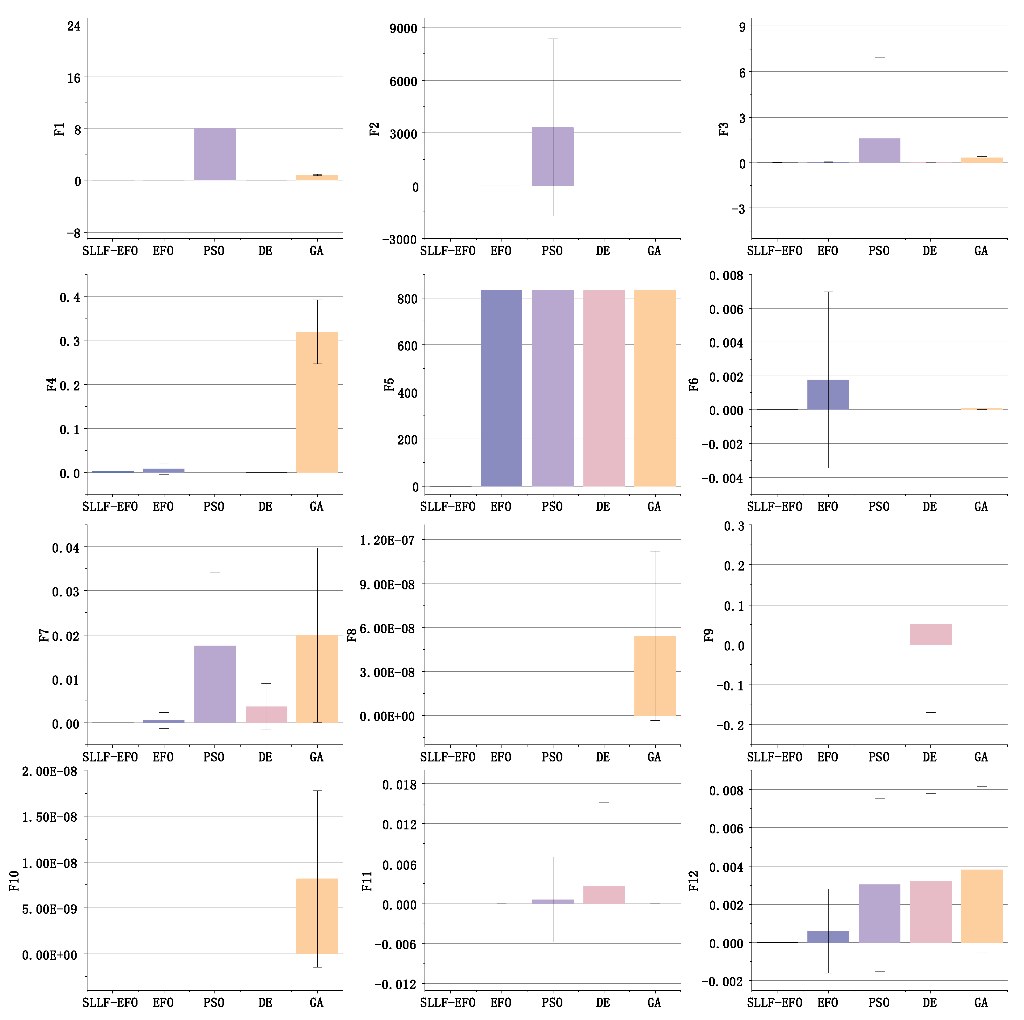
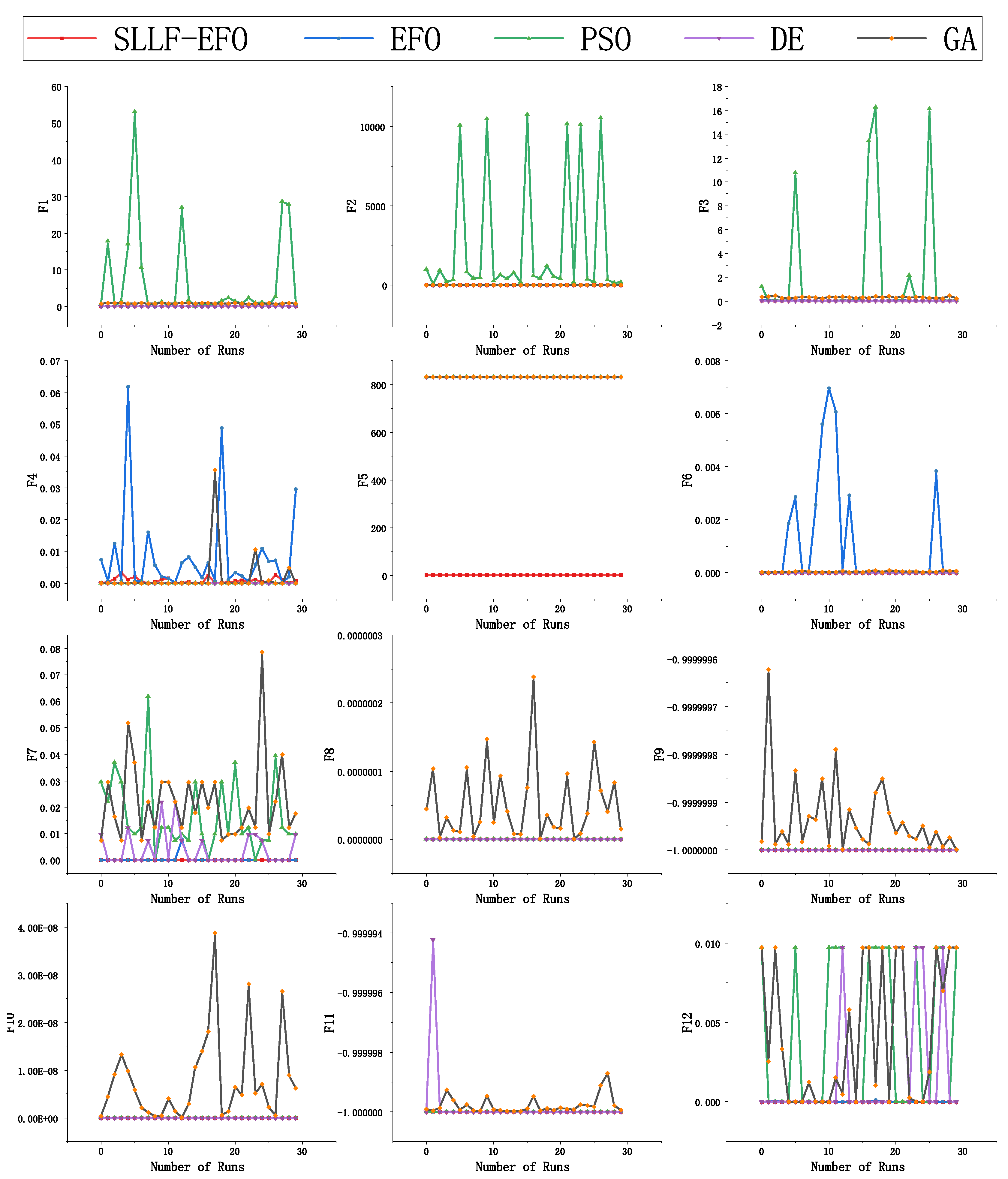
The error bands of 100 experimental results of five algorithms under different test functions are shown in Figure 6. The bands illustrate the stability and robustness of each algorithm, with narrower bands indicating more consistent performance. The comparison of search results between SLLF-EFO algorithm and EFO algorithm under each function is shown in Table 3. The last column in the table calculates the ratio of the average fitness values and standard deviation of EFO algorithm and SLLF-EFO algorithm in all function environments where the optimal solution cannot be successfully found, which is conducive to demonstrating the optimization ability and stability improvement of SLLF-EFO compared to EFO algorithm. Moreover, in order to more intuitively demonstrate the search stability of the five algorithms, 30 randomly selected test results from 100 experiments were plotted as a line graph as shown in Figure 7. The X-axis represents the number of runs, and the Y-axis represents the fitness values. The plot highlights the variability in performance and the consistency of the SLLF-EFO algorithm compared to the others.
According to Figure 6 and Table 3, it can be seen that under 12 benchmark function environments, the optimization results of the SLLF-EFO algorithm are also significantly better than those of the EFO algorithm, and the theoretical optimal values can be stably searched in F2, F8, F9, F10, and F11 environments. In the low dimensional environment of F8-F12, the optimization results of the SLLF-EFO algorithm are stable and superior to the other three algorithms, which fully demonstrates the optimization adaptability of the SLLF-EFO algorithm in low-dimensional environments. In the high-dimensional environment of F1-F7, except for a few cases (such as F4), SLLF-EFO can also achieve high accuracy.
The results of the F5 function in Table 3 show that the convergence results of the other four algorithms are the same, with a standard deviation of 0, indicating that in 100 repeated experiments, the F5 function will cause all algorithms to quickly fall into local optima in the early stages of iteration. However, SLLF-EFO relied on the standstill label strategy to jump out of the initial local optimum and ultimately obtained quite good search results. The other four algorithms, due to the lack of solutions to fall into local optima, always stagnated at the initial local optimum and did not move, resulting in unsatisfactory search results. This further demonstrates the advantages of the standstill label strategy in this paper.
By comparing the ratio data of the “Mean” metric between the SLLF-EFO and the original EFO, the experimental results of the SLLF-EFO show a stable improvement compared to the EFO, with a minimum ratio of 1.13. In the F6 and F7 environments, the average fitness value of the SLLF-EFO has increased by 10 and 8 orders of magnitude, respectively, compared to the EFO.
From Figure 6, it is evident that both the optimization results and the standard deviation of SLLF-EFO are at a relatively low level. Observing Figure 7, among the 30 randomly selected test results, PSO and GA exhibit strong instability in most cases, while EFO and DE also exhibit instability in some functions. The line fluctuation of SLLF-EFO is always smooth and has strong robustness, which also confirms the error band distribution in Figure 6 and is reflected in the Std ratio indicator in Table 3. Looking only at the function environment that has not reached the global optimum, the standard deviation ratio between EFO and SLLF-EFO is still the lowest at 6.98, and it exhibits extremely high stability compared to EFO in F6, F7, and F12 environments. This fully indicates that the improved SLLF-EFO algorithm greatly improves the global optimization effect and stability of EFO.

5. Conclusion

As a new type of meta-heuristic algorithm, the optimization exploration of the EFO algorithm holds significant research value and reference importance. This article analyzes and tests the EFO algorithm, identifying issues such as premature convergence in complex environments, and proposes innovative solutions to these problems. The proposed SLLF-EFO algorithm integrates optimization techniques from multiple EFO algorithms, such as the theory of good point sets, variable step size Levy flight strategy, and stagnation marking strategy, to systematically enhance the optimization performance of the EFO algorithm.
The analysis of simulation test results based on standard test functions reveals that the SLLF-EFO algorithm substantially improves convergence speed, accuracy, and stability compared to the EFO algorithm. The enhanced convergence speed of the SLLF-EFO can be attributed to its use of a good point set for population initialization, ensuring an even distribution of the initial population across the entire search space. Additionally, the algorithm employs an adaptive global range strategy that rapidly reduces the search area, facilitating the identification of the approximate direction of the global optimal solution during the global search phase.
Regarding solution accuracy and stability, the SLLF-EFO incorporates an optimized individual selection strategy for active electric field localization, enhancing the uniformity of population distribution throughout the iteration process. In the passive electric field localization phase, the algorithm integrates the Levy flight search strategy with a variable step size, increasing the algorithm’s stochasticity and jumping ability, addressing problem (3) as outlined in Section 2.2. Furthermore, the introduction of the golden sine strategy enhances population diversity, while the use of the standstill label strategy reduces the number of iterations and facilitates escaping local optima, effectively resolving problems (1) and (2) highlighted in Section 2.2.
Consequently, the SLLF-EFO demonstrates robust global search capability and adaptability to various environments, outperforming the EFO in terms of solution accuracy, stability, and superiority over other meta-heuristic algorithms in diverse settings.
This article addresses the optimization research of the EFO algorithm with the objective of resolving the issue of passive electric field localization stagnation. It also enhances the optimization capability of the EFO algorithm, enabling it to effectively navigate diverse and complex environmental conditions. Potential future research directions include exploring the integration of other meta-heuristic algorithms to further enhance the performance of the EFO algorithm or applying it to complex optimization challenges in various engineering projects. In conclusion, the optimization of the EFO algorithm discussed in this article has substantial implications for guiding future research endeavors involving the EFO algorithm.

Author Contributions

Conceptualization, J.P.; methodology, W.L; software, W.L.; validation, W.L.; formal analysis, W.L. and H.W.; investigation, J.P.; resources, H.W.; data curation, W.L.; writing—original draft preparation, W.L.; writing—review and editing, J.P. All authors have read and agreed to the published version of the manuscript.

Funding

This research was funded by the National Natural Science Foundation of China (Grant No. 62273075) and the Natural Science Foundation of Sichuan Province (Grant No. 2022NSFSC0800).

Institutional Review Board Statement

Not applicable.

Informed Consent Statement

Not applicable

Data Availability Statement

Data are contained within the article.

Acknowledgments

Thanks Professor Jiegang Peng for his guidance on this research, and thank you to the National Natural Science Foundation of China (Grant No. 62273075) and the Natural Science Foundation of Sichuan Province (Grant No. 2022NSFSC0800) for their support of this research work. At the same time, we express our sincere gratitude to all the reviewers who have provided valuable suggestions.

Conflicts of Interest

The authors declare no conflicts of interest. The funders had no role in the design of the study; in the collection, analyses, or interpretation of data; in the writing of the manuscript; or in the decision to publish the results.

References

  1. Darvishpoor, S.; Darvishpour, A.; Escarcega, M.; Hassanalian, M. Nature-inspired algorithms from oceans to space: A comprehensive review of heuristic and meta-heuristic optimization algorithms and their potential applications in drones. Drones 2023, 7, 427. [Google Scholar] [CrossRef]
  2. Yilmaz, S.; Sen, S. Electric fish optimization: A new heuristic algorithm inspired by electrolocation. Neural Computing and Applications 2020, 32, 11543–11578. [Google Scholar] [CrossRef]
  3. Deepa, J.; Madhavan, P. ABT-GAMNet: A novel adaptive Boundary-aware transformer with Gated attention mechanism for automated skin lesion segmentation. Biomedical Signal Processing and Control 2023, 84, 104971. [Google Scholar] [CrossRef]
  4. Ibrahim, R.A.; Abualigah, L.; Ewees, A.A.; Al-Qaness, M.A.; Yousri, D.; Alshathri, S.; Abd Elaziz, M. An electric fish-based arithmetic optimization algorithm for feature selection. Entropy 2021, 23, 1189. [Google Scholar] [CrossRef] [PubMed]
  5. Kumar, M.S.; Karri, G.R. Eeoa: Cost and energy efficient task scheduling in a cloud-fog framework. Sensors 2023, 23, 2445. [Google Scholar] [CrossRef] [PubMed]
  6. Rao, Y.S.; Madhu, R. Hybrid dragonfly with electric fish optimization-based multi user massive MIMO system: Optimization model for computation and communication power. Wireless Personal Communications 2021, 120, 2519–2543. [Google Scholar] [CrossRef]
  7. Anirudh Reddy, R.; Venkatram, N. Intelligent energy efficient routing in wireless body area network with mobile sink nodes using horse electric fish optimization. Peer-to-Peer Networking and Applications, 2024; 1–25. [Google Scholar]
  8. Viswanadham, Y.V.R.S.; Jayavel, K. Design & Development of Hybrid Electric Fish-Harris Hawks Optimization-Based Privacy Preservation of Data in Supply Chain Network with Block Chain Technology. International Journal of Information Technology & Decision Making, 2023; 1–32. [Google Scholar]
  9. Yılmaz, S.; Sen, S. Classification with the electric fish optimization algorithm. 2020 28th Signal Processing and Communications Applications Conference (SIU). IEEE, 2020, pp. 1–4.
  10. Yıldız, Y.A.; Akkaş, Ö.P.; Saka, M.; Çoban, M.; Eke, İ. Electric fish optimization for economic load dispatch problem. Niğde Ömer Halisdemir Üniversitesi Mühendislik Bilimleri Dergisi, 13, 1–1.
  11. Vaishnavi, T.; Sheeba Joice, C. A novel self adaptive-electric fish optimization-based multi-lane changing and merging control strategy on connected and autonomous vehicle. Wireless Networks 2022, 28, 3077–3099. [Google Scholar] [CrossRef]
  12. Pandey, H.M.; Chaudhary, A.; Mehrotra, D. A comparative review of approaches to prevent premature convergence in GA. Applied Soft Computing 2014, 24, 1047–1077. [Google Scholar] [CrossRef]
  13. Nakisa, B.; Ahmad Nazri, M.Z.; Rastgoo, M.N.; Abdullah, S. A survey: Particle swarm optimization based algorithms to solve premature convergence problem. Journal of Computer Science 2014, 10, 1758–1765. [Google Scholar] [CrossRef]
  14. Li, Y.; Lin, X.; Liu, J. An improved gray wolf optimization algorithm to solve engineering problems. Sustainability 2021, 13, 3208. [Google Scholar] [CrossRef]
  15. Engelbrecht, A.P. Particle swarm optimization: Global best or local best? 2013 BRICS congress on computational intelligence and 11th Brazilian congress on computational intelligence. IEEE, 2013; 124–135. [Google Scholar]
  16. Islam, S.M.; Das, S.; Ghosh, S.; Roy, S.; Suganthan, P.N. An adaptive differential evolution algorithm with novel mutation and crossover strategies for global numerical optimization. IEEE Transactions on Systems, Man, and Cybernetics, Part B (Cybernetics) 2011, 42, 482–500. [Google Scholar] [CrossRef] [PubMed]
  17. Hua, L. The application of number theory in approximate analysis. Science Press, 1978; 1–99. [Google Scholar]
  18. ZHANG L, Z.B. Good Point Set Based Genetic Algorithm. CHINESE JOURNAL OF COMPUTERS-CHINESE EDITION- 2001, 24, 917–922. [Google Scholar]
  19. Chen, Y.X.; Liang, X.M.; Huang, Y. Improved quantum particle swarm optimization based on good-point set. Journal of Central South University (Science and Technology) 2013, 4, 1409–1414. [Google Scholar]
  20. Tanyildizi, E.; Demir, G. Golden sine algorithm: A novel math-inspired algorithm. Advances in Electrical & Computer Engineering 2017, 17. [Google Scholar]
  21. Zhang, J.; Wang, J.S. Improved whale optimization algorithm based on nonlinear adaptive weight and golden sine operator. IEEE Access 2020, 8, 77013–77048. [Google Scholar] [CrossRef]
  22. Xie, W.; Wang, J.S.; Tao, Y. Improved black hole algorithm based on golden sine operator and levy flight operator. IEEE Access 2019, 7, 161459–161486. [Google Scholar] [CrossRef]
  23. Drysdale, P.; Robinson, P. Lévy random walks in finite systems. Physical Review E 1998, 58, 5382. [Google Scholar] [CrossRef]
  24. Liu, Y.; Cao, B. A novel ant colony optimization algorithm with Levy flight. Ieee Access 2020, 8, 67205–67213. [Google Scholar] [CrossRef]
  25. Heidari, A.A.; Pahlavani, P. An efficient modified grey wolf optimizer with Lévy flight for optimization tasks. Applied Soft Computing 2017, 60, 115–134. [Google Scholar] [CrossRef]
  26. Gong Ran, Shi Wenjuan, Z.Z. Optimization Algorithm for Slime Mould Based on Chaotic Mapping and Levy Flight. Computer & Digital Engineering 2023, 51, 361–367. [Google Scholar]
  27. Mantegna, R.N. Fast, accurate algorithm for numerical simulation of Levy stable stochastic processes. Physical Review E 1994, 49, 4677. [Google Scholar] [CrossRef] [PubMed]
  28. Bacaër, N. Verhulst and the logistic Equation (1838). A short history of mathematical population dynamics, 2011; 35–39. [Google Scholar]
  29. Kyurkchiev, N. A family of recurrence generated sigmoidal functions based on the Verhulst logistic function. Some approximation and modelling aspects. Biomath Communications 2016, 3. [Google Scholar] [CrossRef]
  30. Ma, Y.N.; Gong, Y.J.; Xiao, C.F.; Gao, Y.; Zhang, J. Path planning for autonomous underwater vehicles: An ant colony algorithm incorporating alarm pheromone. IEEE Transactions on Vehicular Technology 2018, 68, 141–154. [Google Scholar] [CrossRef]
  31. Castillo-Villar, K.K. Metaheuristic algorithms applied to bioenergy supply chain problems: theory, review, challenges, and future. Energies 2014, 7, 7640–7672. [Google Scholar] [CrossRef]
  32. Abdel-Basset, M.; Abdel-Fatah, L.; Sangaiah, A.K. Metaheuristic algorithms: A comprehensive review. Computational intelligence for multimedia big data on the cloud with engineering applications, 2018; 185–231. [Google Scholar]
  33. Nadimi-Shahraki, M.H.; Taghian, S.; Mirjalili, S. An improved grey wolf optimizer for solving engineering problems. Expert Systems with Applications 2021, 166, 113917. [Google Scholar] [CrossRef]
  34. Liu, B.; Wang, L.; Jin, Y.H.; Tang, F.; Huang, D.X. Improved particle swarm optimization combined with chaos. Chaos, Solitons & Fractals 2005, 25, 1261–1271. [Google Scholar]
  35. Guo, W.; Liu, T.; Dai, F.; Xu, P. An improved whale optimization algorithm for forecasting water resources demand. Applied Soft Computing 2020, 86, 105925. [Google Scholar] [CrossRef]
  36. Kennedy, J.; Eberhart, R. Particle swarm optimization. Proceedings of ICNN’95-international conference on neural networks. ieee, 1995; Vol. 4, 1942–1948. [Google Scholar]
  37. Price, K.V. Differential evolution. Handbook of optimization: From classical to modern approach, 2013; 187–214. [Google Scholar]
  38. Holland, J.H. Adaptation in natural and artificial systems: An introductory analysis with applications to biology, control, and artificial intelligence, 1992.
  39. Jamil, M.; Yang, X.S. A literature survey of benchmark functions for global optimisation problems. International Journal of Mathematical Modelling and Numerical Optimisation 2013, 4, 150–194. [Google Scholar] [CrossRef]
  40. Li, F.; Guo, W.; Deng, X.; Wang, J.; Ge, L.; Guan, X. A hybrid shuffled frog leaping algorithm and its performance assessment in Multi-Dimensional symmetric function. Symmetry 2022, 14, 131. [Google Scholar] [CrossRef]
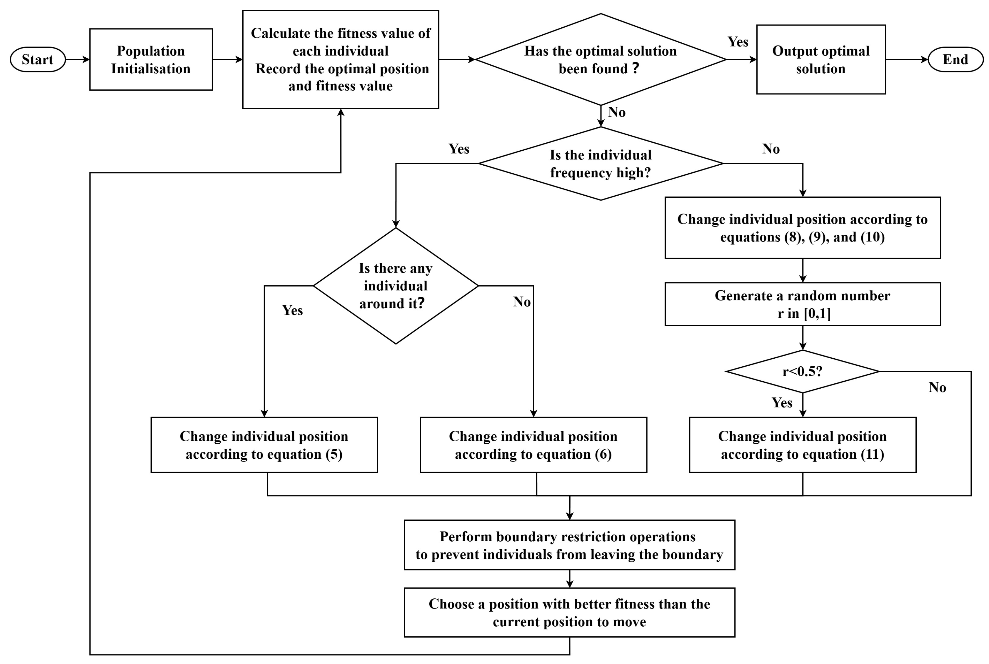
Figure 1. Basic process of electric fish optimization algorithm.
Preprints 118216 g001
Figure 2. Optimization plan for electric fish optimization algorithm.
Preprints 118216 g002
Figure 3. Population distribution of the good point set method and random method.
Preprints 118216 g003
Figure 4. Random walk trajectories of Levy flight and Brownian motion.
Preprints 118216 g004
Figure 5. Convergence curves of 5 algorithms under 12 benchmark test functions.
Preprints 118216 g005
Figure 6. Error bands of search results for each algorithm under 12 standard test functions.
Preprints 118216 g006
Figure 7. 30 repeated experimental test results.
Preprints 118216 g007
Table 1. Benchmark test functions.
Serial Number Functin Search Scope Dimension Optimum Value
F1 Sphere [-5.12,5.12] 30 0
F2 Step [-100,100] 30 0
F3 Quartic [-1.28,1.28] 30 0
F4 Rosenbrock [-5,10] 30 0
F5 Schwefel [-500,500] 30 0
F6 Ackley [-32,32] 30 0
F7 Griewank [-600,600] 30 0
F8 Bohachevsky [-100,100] 2 0
F9 Easom [-100,100] 2 -1
F10 Rastrigin [-5.12,5.12] 2 0
F11 Drop-Wave [-5.12,5.12] 2 -1
F12 Schaffer N6 [-10,10] 2 0
Table 2. Comparison of speed of various algorithms under 12 functions.
Function Index SLLF-EFO EFO PSO DE GA SIF
F1 Exceed Exceed Exceed Exceed Exceed
F2 Min-Iter 62 1005 2000 481 361 13.64
Max-Iter 441 2000 2000 572 827
Mean-Iter 112.17 1530.15 2000 540.34 502.61
Over-Num 0 4 100 0 0
F3 Exceed Exceed Exceed Exceed Exceed
F4 Min-Iter 2000 2000 831 2000 2000
Max-Iter 2000 2000 1291 2000 2000
Mean-Iter 2000 2000 1009.67 2000 2000
Over-Num 100 100 0 100 100
F5 Exceed Exceed Exceed Exceed Exceed
F6 Min-Iter 730 938 797 379 2000 1.57
Max-Iter 2000 2000 1158 464 2000
Mean-Iter 994.52 1563.65 1005.98 422.67 2000
Over-Num 6 31 0 0 100
F7 Min-Iter 327 781 804 410 2000 1.32
Max-Iter 2000 2000 2000 2000 2000
Mean-Iter 1350.48 1789.35 1875.16 1093.83 2000
Over-Num 13 68 88 40 100
F8 Min-Iter 109 157 514 207 2000 1.90
Max-Iter 139 801 1074 283 2000
Mean-Iter 122.51 223.23 798.59 250.04 2000
Over-Num 0 0 0 0 100
F9 Min-Iter 375 803 529 259 2000 2.33
Max-Iter 1483 1970 1007 2000 2000
Mean-Iter 596.18 1388.08 773.71 431.93 2000
Over-Num 0 0 0 5 100
F10 Min-Iter 105 187 517 181 2000 2.00
Max-Iter 229 756 1054 260 2000
Mean-Iter 140.89 281.13 761.67 226.42 2000
Over-Num 0 0 0 0 100
F11 Min-Iter 162 403 506 371 2000 3.30
Max-Iter 582 2000 2000 2000 2000
Mean-Iter 263.02 868.33 771.86 550.53 2000
Over-Num 0 10 1 4 100
F12 Min-Iter 302 931 585 510 2000 2.38
Max-Iter 2000 2000 2000 2000 2000
Mean-Iter 796.27 1894.89 1218.83 1263.89 2000
Over-Num 4 72 31 33 100
Table 3. Search results for 12 types of functions.
Functions Index SLLF-EFO EFO PSO DE GA Ratio
F1 Mean 4.60575 × 10 7 4.85313 × 10 5 8.078069590 2.45612 × 10 16 0.801900988 105.37
Std 9.74995 × 10 7 3.05088 × 10 5 14.08101851 1.893150 × 10 16 0.116547399 31.29
F2 Mean 0 0.04 3306.32 0 0 Extremely High
Std 0 0.196946386 5036.425121 0 0 Extremely High
F3 Mean 0.003147740 0.038953813 1.582964707 0.026996480 0.326350667 12.38
Std 0.001781311 0.012436167 5.361322043 0.006638658 0.067290692 6.98
F4 Mean 0.000854922 0.007367849 0 7.45493 × 10 21 0.319380700 8.62
Std 0.000884378 0.012963790 0 5.48703 × 10 20 0.073208760 14.66
F5 Mean 2.54551 × 10 5 831.8099376 831.8099376 831.8099376 831.8099376 3.27 × 10 7
Std 2.26102 × 10 14 0 0 0 0
F6 Mean 2.84217 × 10 16 0.001767313 0 0 3.99185 × 10 5 6.22 × 10 10
Std 1.20346 × 10 15 0.005219645 0 0 2.27945 × 10 5 4.33 × 10 12
F7 Mean 8.43037 × 10 13 0.000504985 0.017456368 0.003697774 0.019963270 5.99 × 10 8
Std 8.35483 × 10 12 0.001886713 0.016805818 0.005273292 0.019810354 2.26 × 10 8
F8 Mean 0 0 0 0 5.41664 × 10 8
Std 0 0 0 0 5.76108 × 10 8
F9 Mean -1 -1 -1 -0.95 -0.999999957
Std 0 0 0 0.219042914 4.36475 × 10 8
F10 Mean 0 0 0 0 8.15796 × 10 9
Std 0 0 0 0 9.64681 × 10 9
F11 Mean -1 -0.999999843 -0.999362453 -0.997449813 -0.999999729 Extremely High
Std 0 1.46723 × 10 6 0.006375467 0.012556252 3.38904 × 10 7 Extremely High
F12 Mean 4.71959 × 10 12 0.000614620 0.003011932 0.003206250 0.003819688 1.30 × 10 8
Std 4.70359 × 10 11 0.002198893 0.004516180 0.004591560 0.004323915 4.67 × 10 7
Disclaimer/Publisher’s Note: The statements, opinions and data contained in all publications are solely those of the individual author(s) and contributor(s) and not of MDPI and/or the editor(s). MDPI and/or the editor(s) disclaim responsibility for any injury to people or property resulting from any ideas, methods, instructions or products referred to in the content.
Copyright: This open access article is published under a Creative Commons CC BY 4.0 license, which permit the free download, distribution, and reuse, provided that the author and preprint are cited in any reuse.
Prerpints.org logo

Preprints.org is a free preprint server supported by MDPI in Basel, Switzerland.

Subscribe

© 2024 MDPI (Basel, Switzerland) unless otherwise stated