1. Introduction
Convection plays a crucial role in atmospheric circulation, transferring heat from the earth surface to the upper atmosphere, creating vertical air movement to mix air at different altitudes, driving cloud formation and extreme precipitation, shaping the global mass, momentum, and energy budget. Meanwhile, current numerical models fail to explicitly resolve convection processes, due to resolution limits posed by computational constraints. This makes it instrumental to include parameterization schemes that empirically account for the effects of convection, based on the resolved variables of numerical model.
Traditional convection parameterization schemes, coming with error-prone empirical function forms and free parameters, may introduce significant errors in estimating heating, moistening, and precipitation rate at grid scale [
1,
2], which translates to errors in simulated large-scale circulation patterns, such as intertropical convergence zone, Madden-Julian oscillation, and mesoscale convective systems [
3,
4,
5,
6,
7].
A growing interest is to apply high-fidelity data, including high-resolution simulations and observations, to calibrate existing convection schemes, or to develop data-driven simulators using deep neural network. The latter provides more flexibility and higher accuracy, promising a breaker to the deadlock of convection parameterization problem [
8,
9]. Up till now, deep neural networks have been tested thoroughly in numerical models under aquaplanet or realistic geography setup, showing its potential to be the next-generation convection scheme [
10,
11,
12,
13,
14,
15,
16,
17,
18,
19,
20].
Yet, the lack of stochasticity by neural-network-based convection schemes will harm the performance of numerical model. Gentine et al. [
9] found heating and moistening tendencies predicted by deep neural network lack variability below 700 hPa. Rasp et al. [
16] showed that the standard deviation of convective heating tendency below 700 hPa in multi-year simulations is significantly lower after the same neural network is integrated in numerical model. Moreover, traditional stochastic parameterization schemes can improve the ensemble prediction skill and numerical simulation of Madden-Julian oscillation, climate mean, and variability [
21,
22,
23]. It is expected that stochastic parameterization of moist physics by neural network may further improve its performance in numerical models.
Generative model is a kind of deep learning model based on probability theory. It establishes a mapping between a known prior distribution and the target distribution. It is naturally suited for stochastic parameterization. Classic generative models include variational auto encoder (VAE) [
24] and generative adversarial network (GAN) [
25]. GAN was explored in stochastic parameterization of convection, subgrid stress of ocean model, and stochastic tendencies in Lorenz-96 model [
26,
27,
28,
29,
30,
31,
32]. Yet, VAE is hindered by its blurring generated samples and posterior collapse [
33,
34]. GAN suffers from difficulties in training and mode collapse [
35,
36]. Efforts have been made to stabilize the training and secure the diversity and quality of generated samples [
33,
35,
36,
37,
38]. But it still requires strong case-specific experiences to train a good generative model based on GAN and VAE.
Recent years a new family of generative model, probabilistic diffusion model (PDM) [
39], has received special attentions. PDM is the foundation model of the well-known text-to-image models like Stable Diffusion [
40] and Dall-E [
41]. PDM splits the generative task into a series of relatively simple denoising tasks. This paradigm shift makes PDM much easier to train and suffer from much less mode collapse [
39,
42,
43]. PDM shows its strong dominance due to its high quality of generative samples [
44].
In this study, a stochastic parameterization scheme for moist physics based on PDM (DIFF-MP) is developed. A cloud-resolving global simulation is coarse grained into resolved variables and subgrid contributions to form the training data of DIFF-MP. The fatal flaw of PDM is its slow inference speed. Adapted from Chen et al. [
45], we let DIFF-MP train on a series of noised levels in a stochastic way to generalize to large denoising steps for acceleration. Cassifier-free guidance [
46] is used for tuning the influence of conditional information by fusing the denoised latents of conditioned and unconditioned models at inference stage for further improvements of DIFF-MP. DIFF-MP is further compared with GAN and VAE on testing data for stochastic parameterization of moist physics. Finally, the physical interpretability of DIFF-MP is explored.
The remainder of this study is organized as follows.
Section 2 presents the details of cloud-resolving data and scale-separation techniques for training data generation.
Section 3 presents the training details of the DIFF-MP, and how to accelerate DIFF-MP and use classifier-free guidance to improve its performance.
Section 4 presents the testing data performance of DIFF-MP and its comparisons with baselines, GAN and VAE.
Section 4 also discusses the interpretability of DIFF-MP. Finally, section 5 concludes this work and presents future perspectives.
2. Training Data Preprocessing
The training data is diagnosed from high-fidelity data from cloud-resolving simulation based on Global-Regional Integrated forecast SysTem (GRIST) [
47,
48]. GRIST is formulated on primitive equations. The horizontal mesh adopts structured Delaunay-Voronoi grid [
49]. This kind of grid mesh is appropriate for the global simulation due to its isotropic properties. High-fidelity data from high-resolution simulations are widely used for training data of machine-learning based parameterization schemes because most of atmospheric motions including convections are explicitly resolved.
The simulations consist of four periods: 1988.10.1-1988.10.20, 1998.1.1-1998.1.20, 2005.4.1-2005.4.20, and 2013.7.10-2013.7.29, including four seasons with ENSO and MJO events of various intensities. La Nina and El Nino are strong in 1988 and 1998 respectively. MJO are strong in 1988, 1998, and 2005. Those four periods are chosen for diversity of training data. The horizontal resolution of the simulation is 5 km, which is high enough to resolve deep convections. There are 30 levels under 20 km, with extra levels in boundary layer. The initial condition is interpolated from ECMWF Reanalysis v5 (ERA5) [
50]. The boundary condition (sea surface temperature) is updated every 24 hours. GRIST adopts Yonsei University scheme (YSU) [
51] for boundary layer parameterization, Noah-MP land surface model for surface-atmosphere flux parameterization, WRF single-moment 6-class scheme (WSM6) [
52] for microphysics parameterization, and RRTMG shortwave and longwave schemes [
53] for radiation parameterization. Model outputs are saved every modeling hour.
The high-resolution data need to be preprocessed into subgrid contributions and large-scale resolved variables to form the training data. Microphysics and subgrid vertical transports are regarded as the subgrid processes, which are the output of DIFF-MP. They include subgrid vertical transports of heat and water vapor, and four outputs from WSM6 scheme: temperature tendency (), water vapor tendency (), cloud water () and cloud ice mixing ratios (). Rain, snow, graupel mixing ratios, and subgrid vertical transports of and are not considered because they are negligible. Six variables are selected as the conditional input of DIFF-MP: temperature (T), water vapor mixing ratio (), surface pressure (), sensible heat flux (), latent heat flux (), and short-wave radiation at surface (SOLIN). The procedure to process high-resolution data is shown as follows.
A random group of points on high-resolution Delaunay-Voronoi grid that are seamlessly connected are chosen for coarse graining and subgrid diagnosing. Those points are labeled as
,
,
, …,
. Those
points must try their best to form a regular hexagon or pentagon. The coarse-grained variable is labeled as
for variable
in high-resolution data, then,
Through coarse graining (equation 1), we can get averaged variables for DIFF-MP’s conditional input and output except for subgrid contributions of
and
. If the difference between
and
is
, then the subgrid vertical flux of
is,
The tendency due to subgrid vertical flux of
is,
According to the definition, the subgrid contributions for
and
are,
The reason why the subgrid contributions are formulated as presented above is explained in supplementary material. The conditional input and output variables for DIFF-MP are shown in
Table 1.
Four resolutions are considered in this study: 120 km, 60 km, 30 km, and 15 km, corresponding to 576, 144, 36, and 9 points in equations 1 and 2. The number of training data for all the four resolutions are the same. The conditional input of DIFF-MP has four variables at surface layer. Those variables are each duplicated vertically for 30 times to align with vertical profiles of
and
to form the input matrix.
and
are normalized by subtracting 0.05-quantile and dividing by the difference between 0.95-quantile (
) and 0.05-quantile (
),
The other conditional input and output variables are normalized by dividing by
,
After normalization, the samples that contain output variable larger than 3.0 are all replaced by the neighboring samples within 3.0 to exclude the abnormal high values. The four simulations have 20 days each. The first day is discarded due to the model spin up. The following 13 days are chosen as training data, 4 days as validation data and final 2 days as testing data. Data from the four periods are randomly mixed, and there are 51,118,080, 15,728,640 and 7,864,320 samples for training, validation and testing data. To accelerate the validation and testing of DIFF-MP, only random 10,000 and 1,600,000 samples of validation and testing data are used.
3. DIFF-MP, Inference Acceleration and Classifier-Free Guidance
3.1. DIFF-MP and Its Training
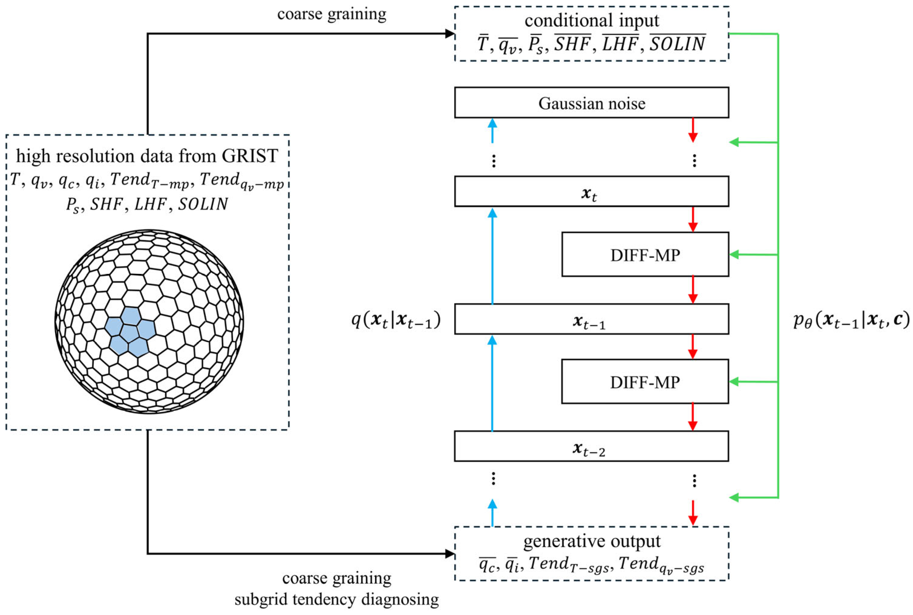
Figure 1 shows how high-resolution data is preprocessed and how DIFF-MP stochastically parameterize moist physics. DIFF-MP can be divided into forward and reverse diffusion processes. In forward diffusion process, target data was fused by gaussian noise step by step until complete noise (blue arrows in
Figure 1). DIFF-MP is trained to reverse forward process stepwise and generate samples in reverse process (red arrows in
Figure 1). A brief introduction to PDM’s mathematic derivations, training and sampling algorithms are presented in supplementary material.
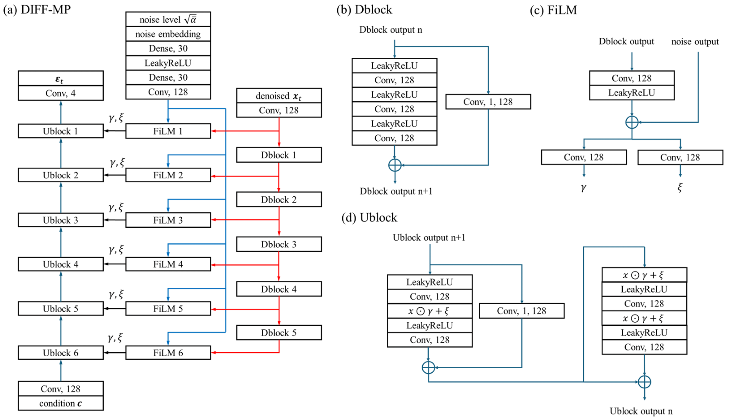
DIFF-MP is a hierarchical one-dimensional PDM, whose structure is depicted in
Figure A1. The number of filters and layers of DIFF-MP are 128 and 6 based on the hyper-parameter experiments. DIFF-MP is inspired by Wavegrad [
45] for network structure, GAN-TTS [
54] for Ublock structure. The feature-wise linear modulation module (FiLM) [
55] is used to combine information from noise level
, denoised
, and conditional input
.
Adam algorithm and cyclical learning rates ranging from 1e-4 to 1e-3 are used for DIFF-MP training [
56,
57]. Loss function is mean squared error. Batch size is 8,000. DIFF-MP is trained for five epochs. Model weights are saved at the end of last epoch. DIFF-MP is trained in Python package Keras 3.0 [
58] on Nvidia 4090 GPU. Different DIFF-MPs are trained on different resolutions for thorough validation of its performance.
3.2. Inference Acceleration of DIFF-MP
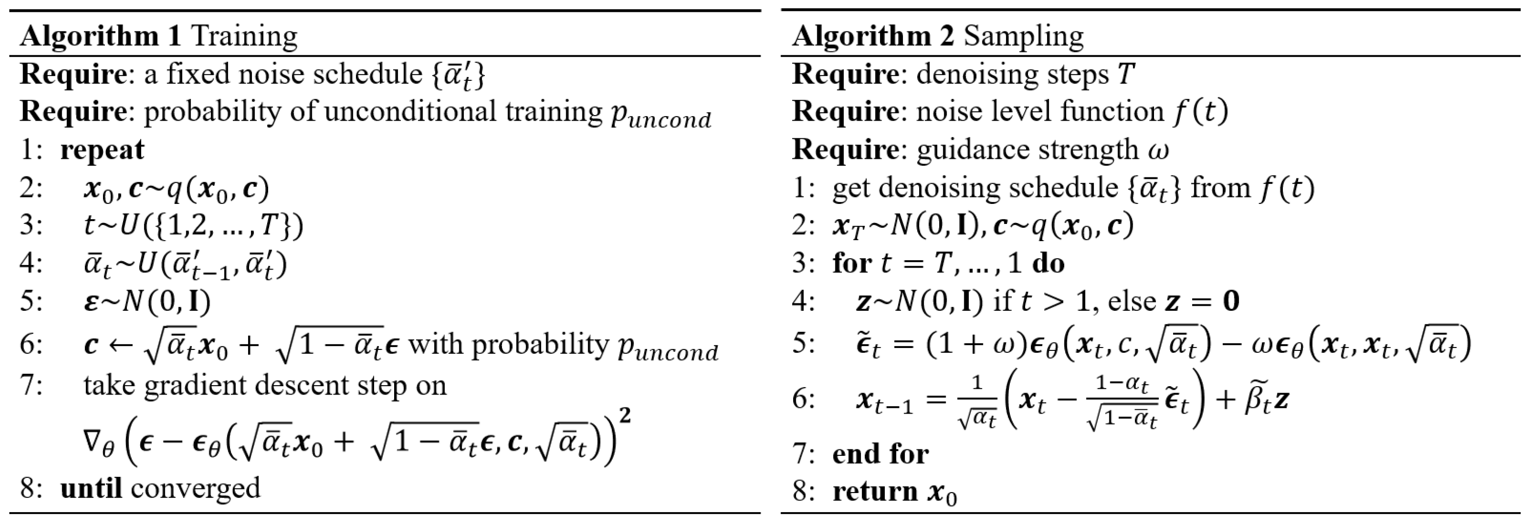
The training and sampling algorithms of DIFF-MP with inference acceleration in detail is presented in
Figure 2. Typically, PDM is only trained on a fixed time-step schedule. When fewer time steps are applied, PDM must follow a quite different denoising route that it is not trained on, leading to degraded performances. To improve the DIFF-MP’s adaptability to fewer denoising steps, it is conditioned on the noise level
directly. This is also adopted by Song and Ermon [
59,
60] in their score matching framework. Moreover,
at time step
is sampled from a uniform distribution
during training. This distribution is defined from a predefined fixed noise schedule
, in which
linearly decreases from 9.9999 to 9.94 with 100 steps. During testing, denoising schedule
is interpolated from noise level function
(
Figure S1), which is constructed from the predefined fixed noise schedule
. Then sampling of DIFF-MP is the same as ordinary PDM. This algorithm is adapted from Chen et al. [
45] with modifications in inference stage.
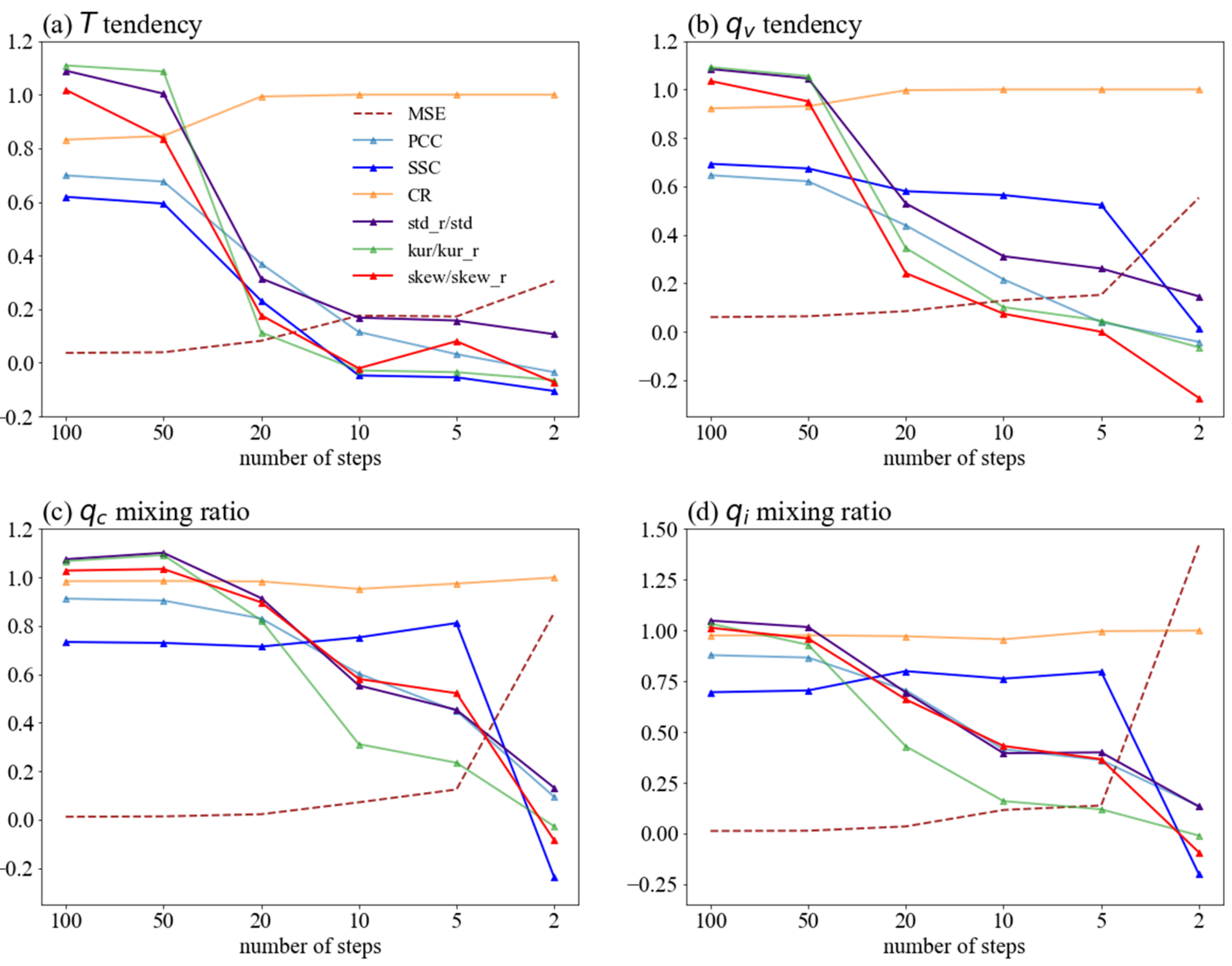
To show the adaptability of DIFF-MP with inference acceleration to different denoising steps, it is compared with DIFF-MPs trained with other fixed steps only. The other DIFF-MPs are trained on fixed noise schedules: linearly decreases from 9.9999 to 9.94, with total time steps of . is set to be 100, 50, 20, 10, 5 and 2. All the models are trained for five epochs until converged. Model weights are saved at the end of last epoch.
Validation criteria are the mean squared error, Pearson correlation coefficient, coverage ratio, spread-skill correlation, standard deviation, kurtosis, and skewness. Because DIFF-MP is a stochastic parameterization scheme, the validation must be conducted on an ensemble of output. For a single conditional input, 32 different outputs are generated. Mean squared error and correlation coefficient measure the error of stochastic parameterization. Coverage ratio is the ratio of validation data that are in the value range of DIFF-MP output ensemble. A good output ensemble should cover the validation data, so DIFF-MP should have high coverage ratio. Spread-skill correlation is the correlation coefficient between the error of DIFF-MP and the spread of DIFF-MP. DIFF-MP should have large spread when it has large prediction error, so DIFF-MP should have high spread-skill correlation. Standard deviation, kurtosis, and skewness measure the high-order statistics of samples generated by DIFF-MP. Those statistics should be close to the corresponding statistics of validation data. How those criteria are calculated are presented in supplementary material.
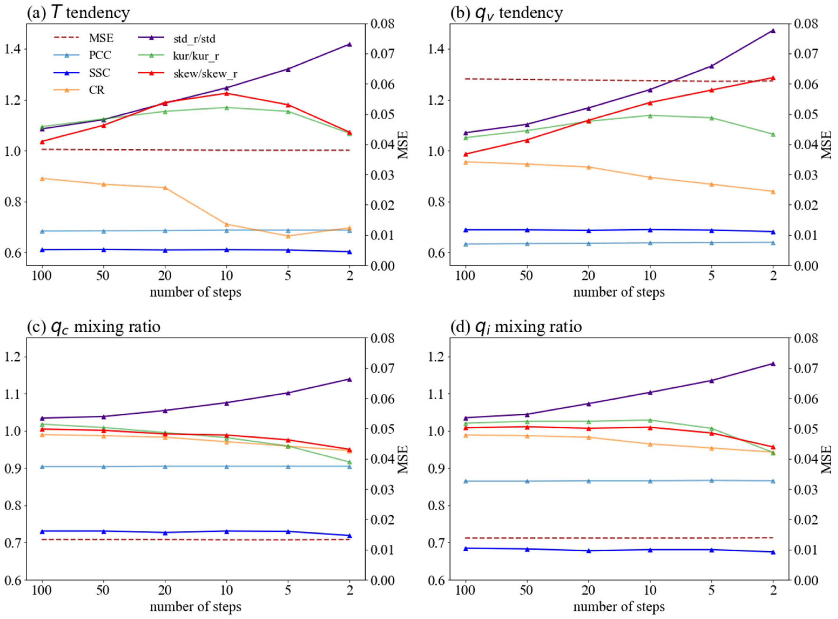
Figure 3 and
Figure 4 show the validation data performance of different DIFF-MPs. Those models are trained on data of resolution 120 km. Results on the other resolutions are similar. For DIFF-MPs trained on fixed steps, their performances degrade quickly as number of steps decreases, except for coverage ratio (
Figure 3). Coverage ratio increases because the sample spread is unreasonably large when denoising steps are too few (
Figure 3). But for DIFF-MP trained with inference acceleration, correlation coefficient, mean squared error, and spread-skill correlation merely change with different steps (
Figure 4). Standard deviation, skewness and kurtosis only deviate from validation data limitedly (
Figure 4). DIFF-MP trained with inference acceleration is significantly better than DIFF-MPs trained on fixed steps. Training on a series of noise levels will effectively alleviate the overfitting of DIFF-MP to limited fixed steps and help its performance generalize to different steps. Consider the balance between the acceleration and sample quality, DIFF-MP in the rest of the study uses five steps to denoise.
3.3. Classifier-Free Guidance of DIFF-MP
Standard deviation, skewness, and kurtosis of samples generated by DIFF-MP deviate from validation data on
and
when DIFF-MP uses five steps to denoise (Figures 4a, b). Standard deviation is also smaller for
and
(
Figure 4c, d). Cassifier-free guidance [
46] can alleviate the deviation of the statistics (standard deviation, skewness, and kurtosis). This method is originally proposed to improve the diversity of generated samples from conditional PDM. When conditional information of PDM is too strong (weak), the samples generated tend to be deterministic (diverse) and the statistics of samples will deviate from original data. Classifier-free guidance fuses the denoised latent from the conditional PDM with the denoised latent from another unconditional PDM. In this way, the statistics of the samples generated by conditional PDM will be drawn closer to the original data.
During training stage, DIFF-MP’s condition input
will be replaced by denoised latent
with a probability of 0.1, through which an unconditional DIFF-MP is trained in the meantime. The final output will be the combination of the denoised latents from the conditional and unconditional DIFF-MPs by mixing ratio
. For each denoising steps,
where
is original DIFF-MP,
is the combined DIFF-MP. The training and sampling algorithms of DIFF-MP using classifier-free guidance and inference acceleration are presented in
Figure 5.
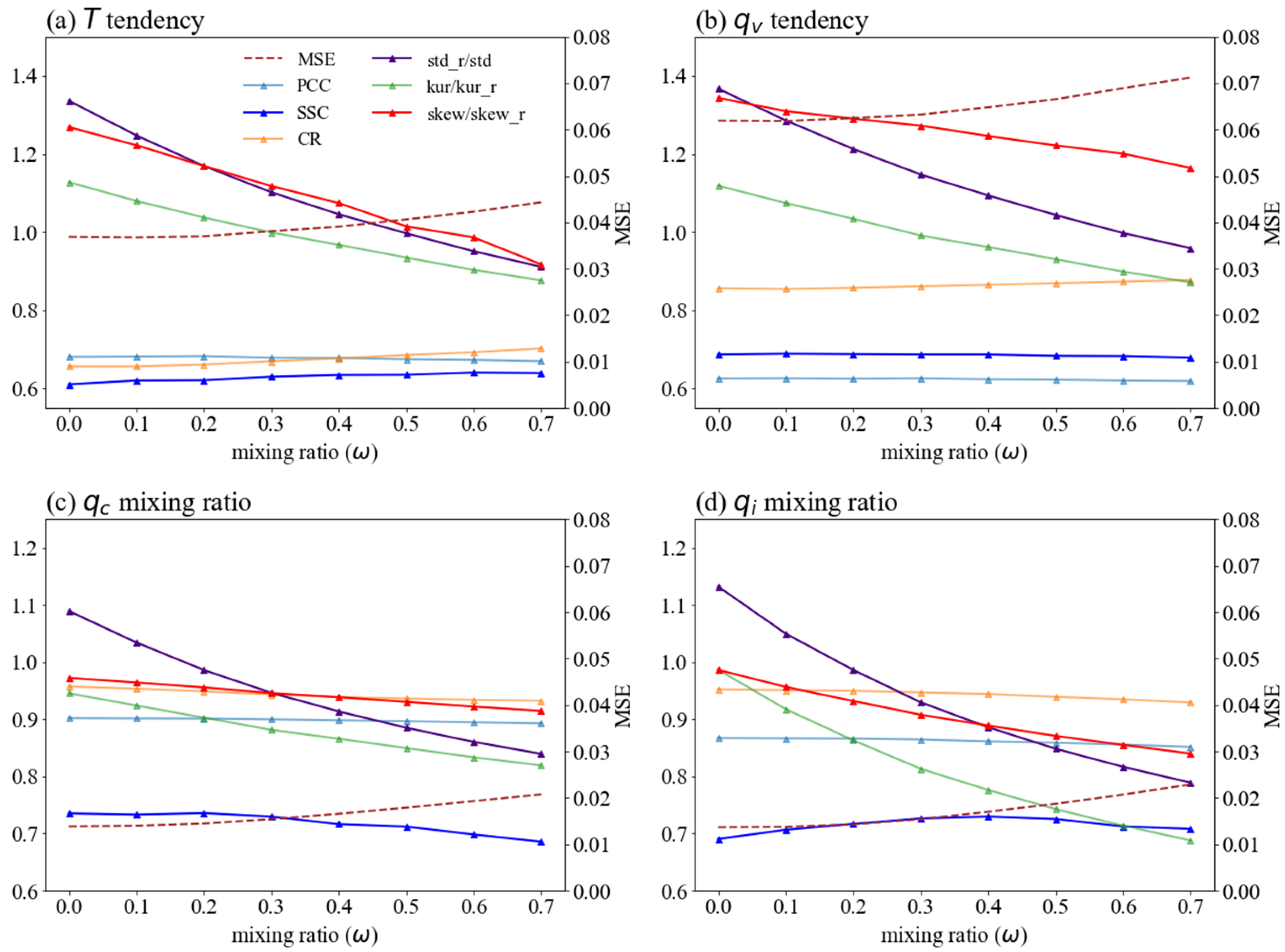
Figure 6 shows the influence of
on DIFF-MP performance on validation data at the resolution of 120 km. As
increases, kurtosis and skewness decrease evidently, but standard deviation increases. Classifier free guidance successfully pushes the statistics of samples generated by DIFF-MP to the validation data. In the meantime, the other four criteria do not change much. The best
for
and
is 0.5. But for
and
, no mixing is better. It is also found that different
for different output variables will not interfere with each other during the inference stage. The same validation of
is also conducted on the other resolutions. The best
for all the four resolutions are in
Table 2, which will be followed by DIFF-MP in this study.
4. Results
4.1. Baseline Models and Their Trainings
Conditional VAE (CVAE-MP) and conditional GAN (CGAN-MP) are selected as baselines. VAE maps each sample from training data into a known distribution within the latent space to form a random coding [
24], which enables the random generation of the training data. GAN is composed of two competing networks, in which generator can produce data that cannot be distinguished from discriminator [
25]. Both models are widely used in generative learning and appropriate for stochastic parameterization of moist physics. Variables in
Table 1 are also used for conditional inputs of CVAE-MP and CGAN-MP. To make a fair comparison between different generative models, DIFF-MP, CVAE-MP, and CGAN-MP have the same model size. Model structures of CGAN-MP and CVAE-MP are presented in
Figures S2 and S3.
Training settings of CVAE-MP and CGAN-MP are the same as DIFF-MP. CGAN-MP output is the sum of a pretrained neural network and the generator. The pretrained neural network predicts the output profiles deterministically, and its weight is frozen during training of CGAN-MP. Wasserstein GAN technique is also applied to stabilize CGAN-MP training [
35]. CVAE-MP and CGAN-MP are trained for 2 and 22 epochs until performance converged. The best models on validation data are saved for further comparison with DIFF-MP on testing data. Validation criterion is the average of correlation coefficient, spread-skill correlation, and coverage ratio. Different models for CVAE-MP and CGAN-MP are also trained for different resolutions.
4.2. Performance Comparison between Models
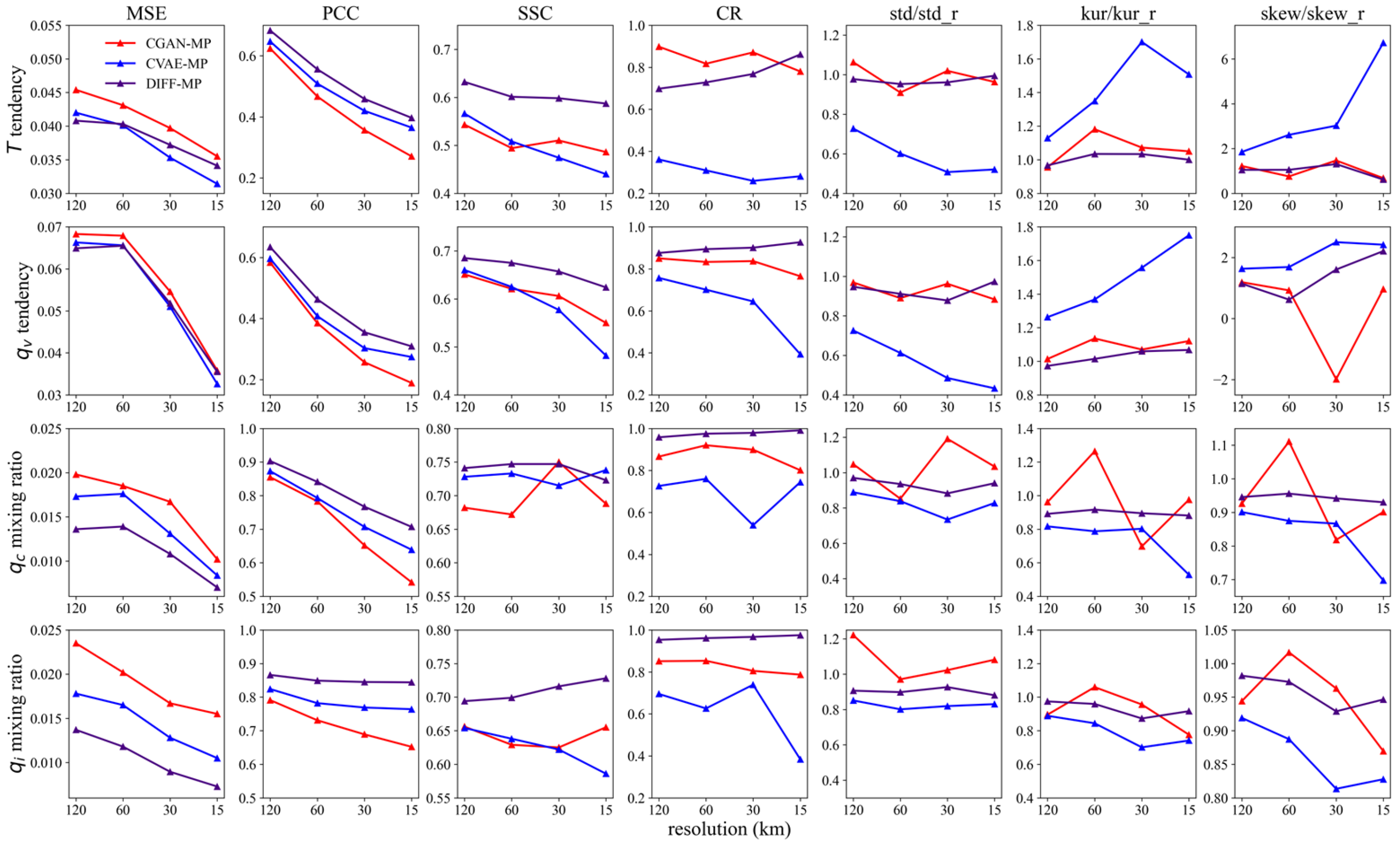
The testing data performance of CGAN-MP, CVAE-MP, and DIFF-MP at different resolutions are presented in
Figure 7. For mean squared error, DIFF-MP is significantly better than the others on
and
, and nearly the best on
and
. DIFF-MP is consistently the best on correlation coefficient and spread-skill correlation. It also beats the other two models on coverage ratio except for
. In terms of the statistics of the samples generated, DIFF-MP is closer to testing data in general than the other two models. It also achieves a much more consistent performance among different resolutions. It is concluded that DIFF-MP performs robustly better than CGAN-MP and CVAE-MP on testing data.
It is noticed that performances of mean squared error and correlation coefficient degrade as resolution increases. This is because as grid spacing increases, coarse graining involves more averaging over turbulences and cloud processes, which makes the subgrid processes more predictable. The same degradation is also reported in other studies [
19,
61].
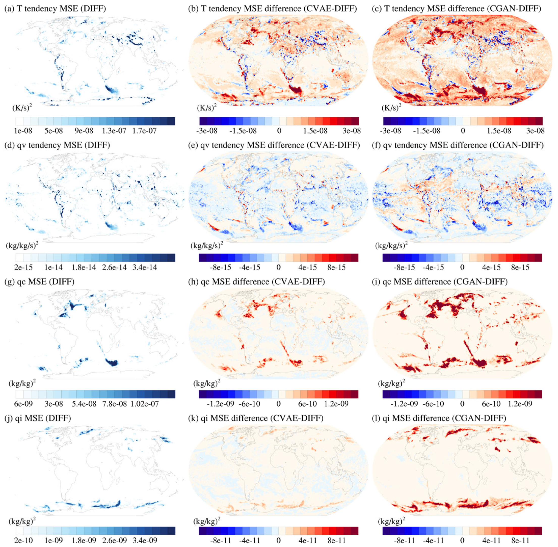
The global distribution of mean squared error by DIFF-MP, and the mean-squared-error differences between models at 120 km resolution are depicted in
Figure 8. DIFF-MP’s mean squared error is mostly distributed in midlatitude where extratropical cyclones are active. Besides, mean squared error of
and
is also distributed along the large-scale terrain and tropical zone where shallow convections are active (Figures 8a, d). Except for
, DIFF-MP has smaller mean squared error than the other two models globally. The red color at background indicates the lower systematic error by DIFF-MP.
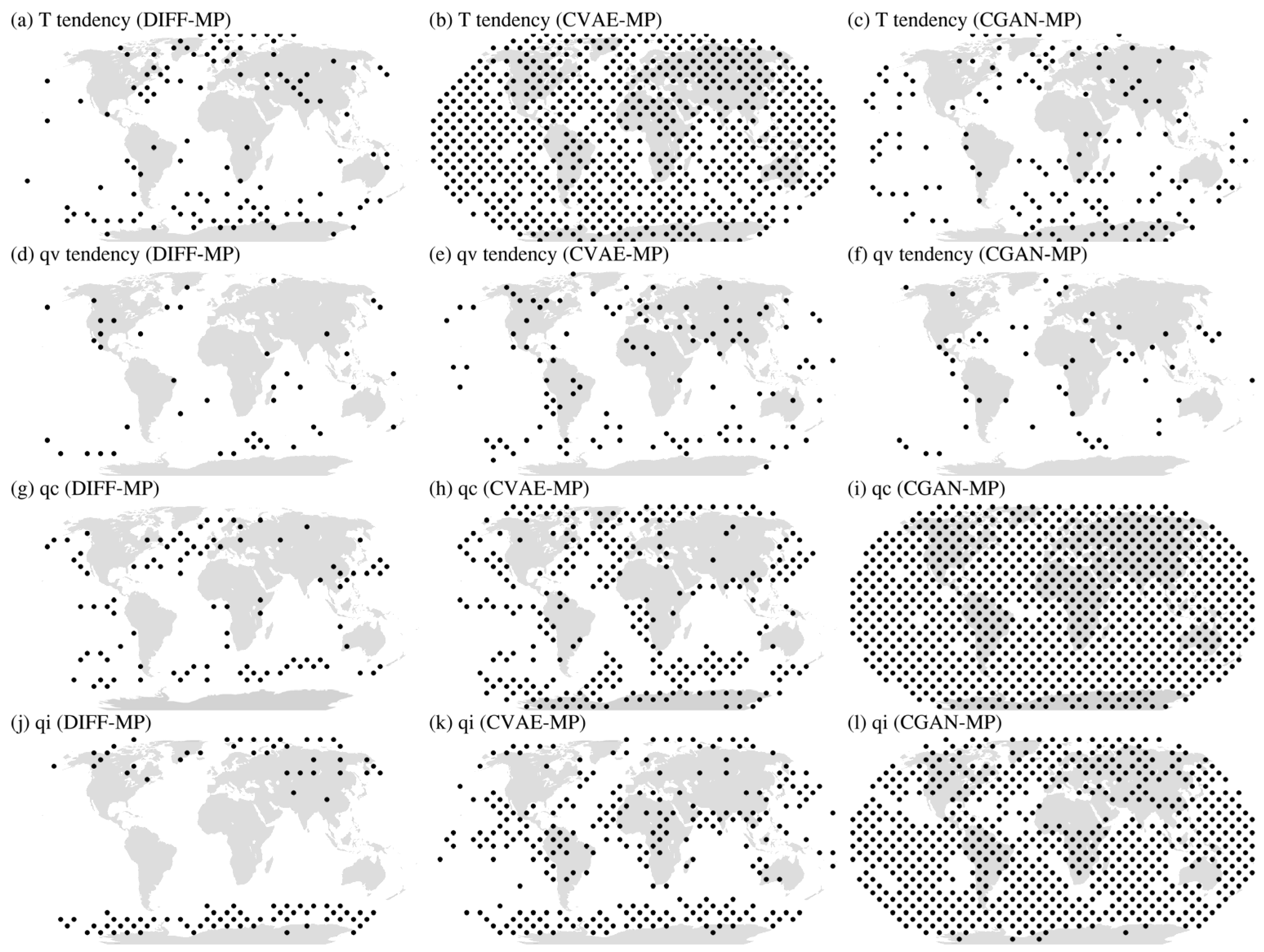
Figure 9 shows the global distribution of whether testing data is in the range of model ensemble at 120 km resolution. DIFF-MP covers almost 90% of testing data for all the variables. The uncovered locations spread along the regions with large mean squared error in
Figure 8. Almost all the testing data of
are not covered by CVAE-MP (
Figure 9b). So are
and
from CGAN-MP (Figures 9i, l).
Figure 8 and
Figure 9 furtherly confirm the robustness of DIFF-MP’s better performance over the other models.
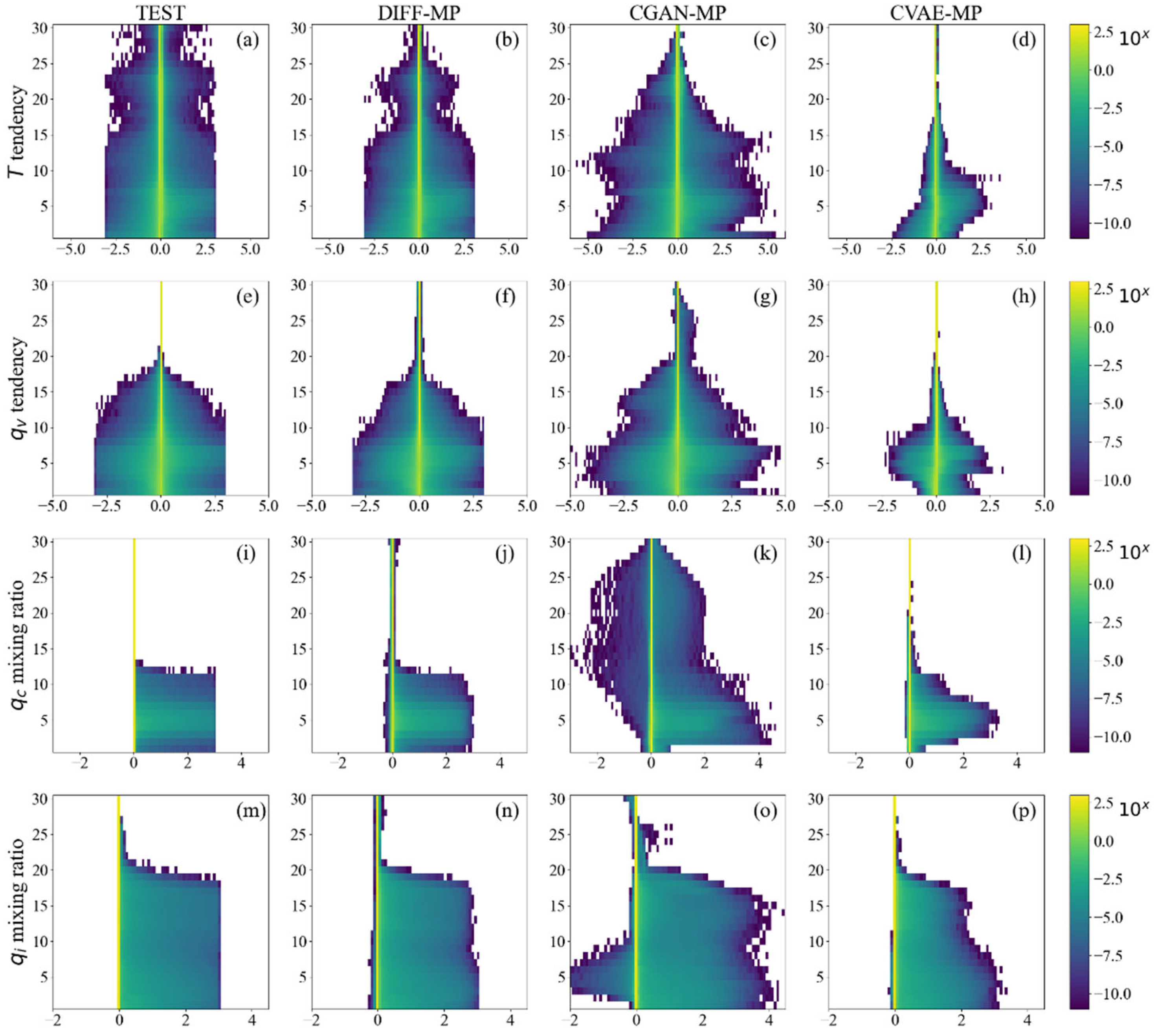
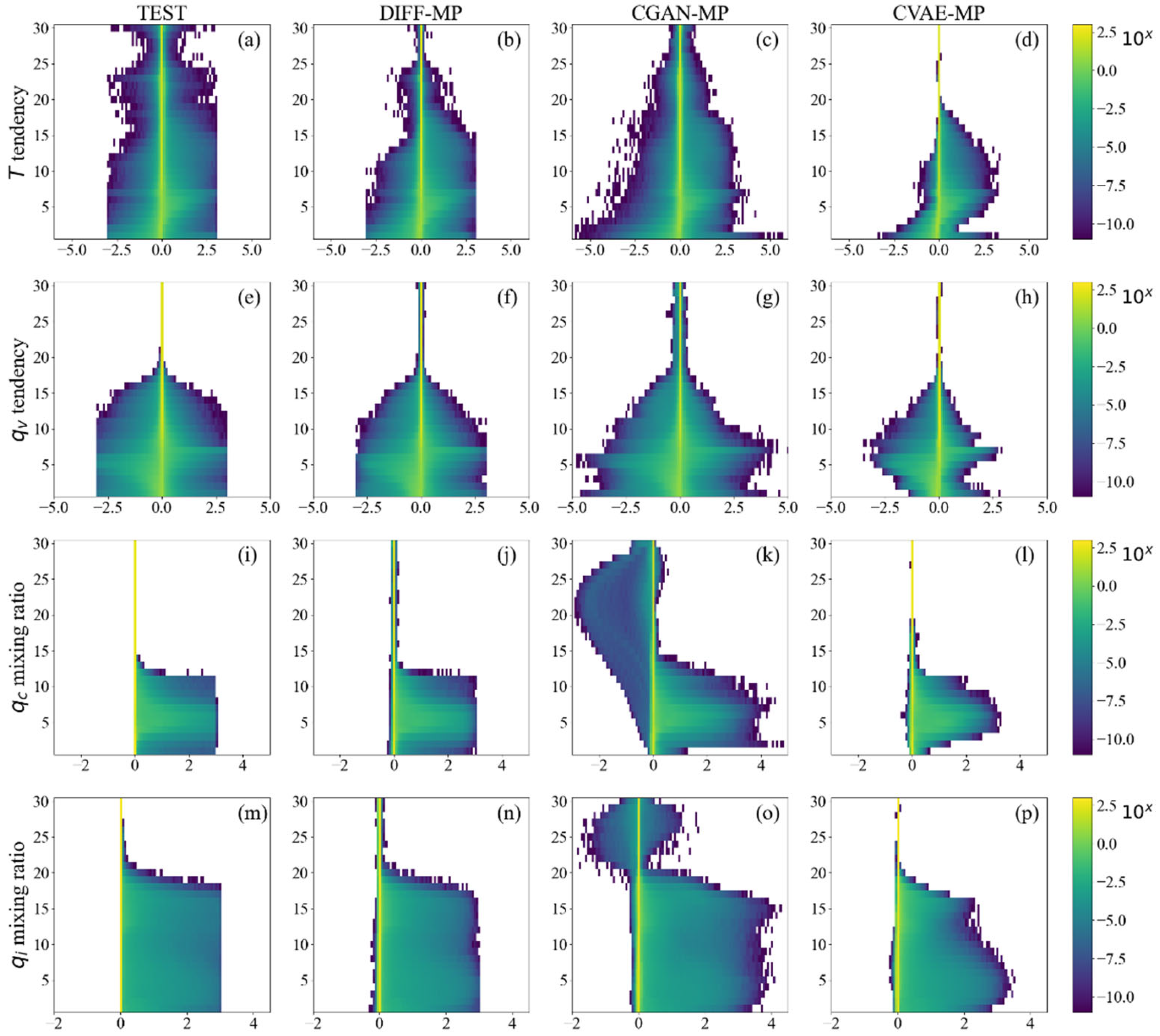
Figure 10 shows the per-level distribution of model generated samples at 120 km resolution. Testing data distributions in
Figure 10 all stop abruptly at -3.0 and 3.0 because abnormal extreme data are excluded. We can see two distinct signals of shallow and deep convections in
Figure 10a.
is mostly positive on upper levels of boundary layer (about level 7), but negative on lower levels. This is due to the condensation of water vapor in shallow convections, where the latent heat is released near the boundary layer top but collected on the lower levels. In
Figure 10e,
is positive near the boundary layer top but negative below, indicating the transport of water vapor by shallow convections. Shallow convections are also shown in lower-level extremes of
and
(Figures 10i, m). Above boundary layer, there is another peak of heating for
on levels 10-15 (
Figure 10a). This is where the deep convections form. Deep convections are also seen in upper levels of
(
Figure 10m).
Signals of shallow and deep convections are generally captured by all three generative models. But the predicted distributions of extreme data are different. DIFF-MP almost perfectly reproduces the data distribution of testing data, even the artificial abrupt at ±3.0. Only the distributions of
above level 15 are underestimated (
Figure 10b). CVAE-MP is overly conservative on extreme values. Only the probability density of large value is captured (Figures 10d, h, l, p). While CGAN-MP is excessively radical, leading to overly large area of probability distributions (Figures 10c, g, k, o). CGAN-MP also predicts unreasonable negative values for
and
.
Figure A2 shows the results from 30 km resolution, which are consistent with
Figure 10.
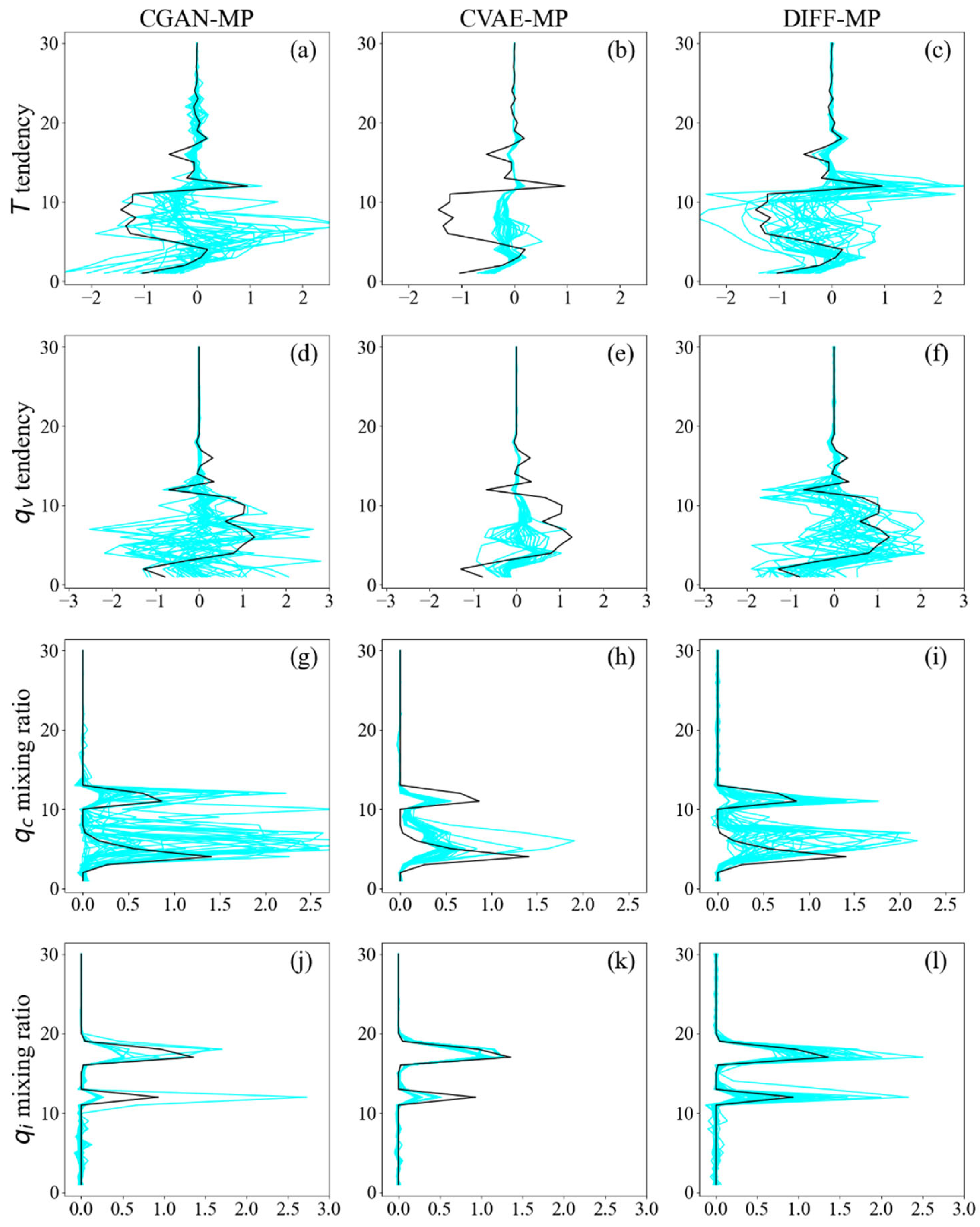
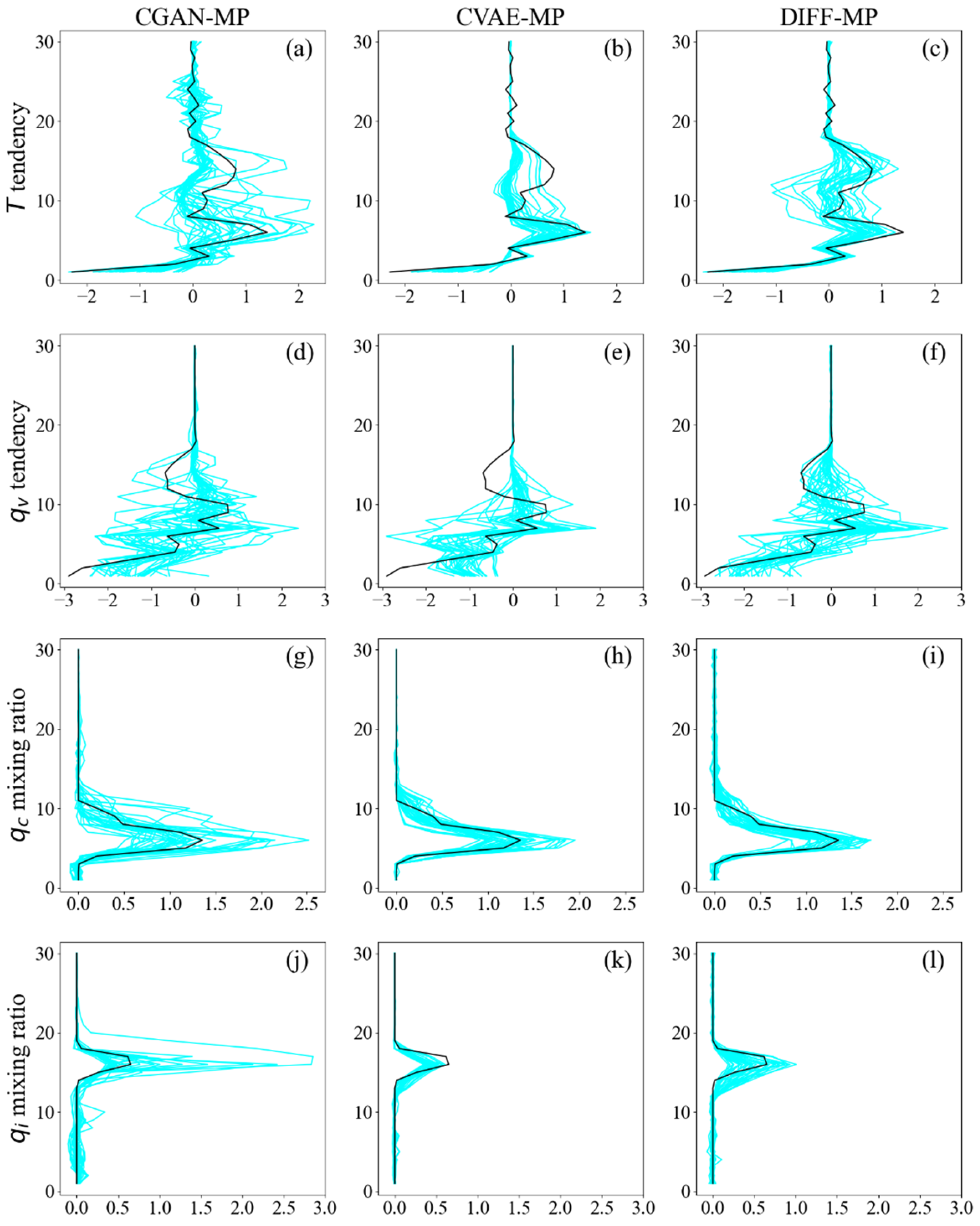
Figure 11 shows the ensemble output profiles from different models and corresponding output profiles from testing data at 120 km resolution. All the models’ ensemble can capture the overall vertical variability of profiles from testing data. But for
and
, CGAN-MP’s and CVAE-MP’s ensembles concentrate about zero value and deviate from testing data on levels 10-15 (Figures 11a, b, d, e). On the contrary, DIFF-MP’s ensemble shares the similar vertical variability as testing data (Figures 11c, f). As for
and
, CGAN-MP’s ensemble extends to 2.0-2.5 (Figures 11g, h). This is also confirmed by
Figure 10 where CGAN-MP predicts excessive extreme values. Value ranges of CVAE-MP’s and DIFF-MP’s ensembles match testing data better than CGAN-MP. Results on 30 km resolution are similar with
Figure 11, which are presented in
Figure A3.
DIFF-MP can recover the data distribution of subgrid moistening, heating, and cloud processes better than CGAN-MP and CVAE-MP. It is also obvious that compared to the other two models, DIFF-MP can produce reasonable ensemble that can cover the output profiles from testing data. DIFF-MP is better than the other two models on the stochastic parameterization of the moist physics.
4.3. Interpretability of DIFF-MP
It is of vital importance to test the interpretability of DIFF-MP to secure the physical robustness.
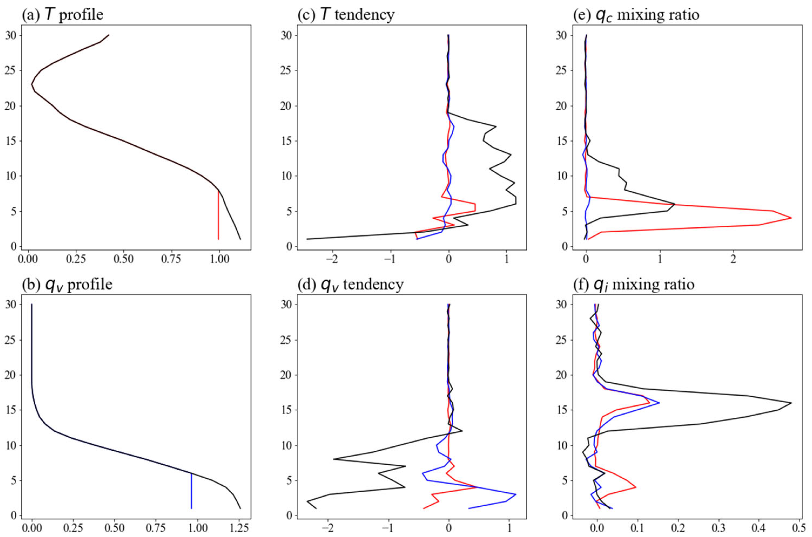
Figure 12 shows the influence on DIFF-MP’s outputs due to the change of stratification in boundary layer. The original boundary layer has unstable stratification. After
profile is neutralized,
and
are almost zero (Figures 12c, d).
on higher levels also decreases, indicating the termination of shallow and deep convections (
Figure 12f).
and
increase in boundary layer (Figures 12e, f). This is because
accumulates in boundary layer due to suppressed convections, which cause excessive condensation. While after
is neutralized,
becomes positive and
disappear in boundary layer (Figures 12d, e). This is because
is not saturated after the neutralization. Therefore, shallow clouds evaporate and
in boundary layer is restored by DIFF-MP.
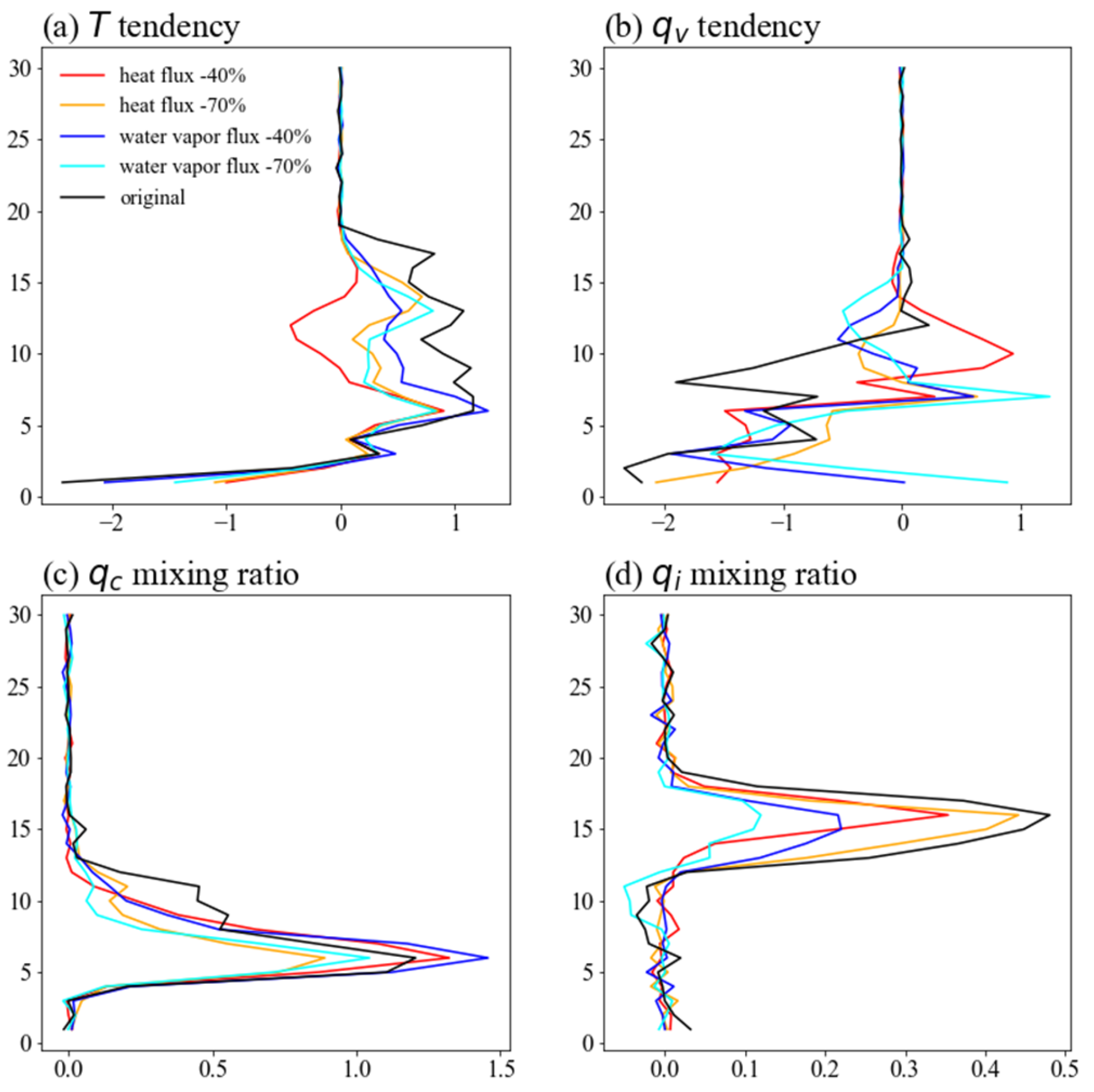
Figure 13 shows the influence of surface flux. As surface flux decreases,
,
, and
on higher levels decrease significantly (Figures 13a, b, d). This is caused by the suppressed deep convections due to surface flux reduction.
in boundary layer increases first and then decreases as surface flux is further reduced. Similar to
Figure 12e,
is first accumulated in boundary layer when convections are constrained. But
is then reduced when convections are severely constrained.
Figure 12 and
Figure 13 confirm that DIFF-MP’s response to the input variation is physically reasonable, which secure the future implementation of DIFF-MP into GRIST model.
5. Conclusions and Discussions
This study develops a stochastic moist physics parameterization scheme named DIFF-MP based on one-dimensional PDM. DIFF-MP is trained on a series of noise levels which boosts its generalizability to large denoising step to accelerate. DIFF-MP achieves 20 times acceleration without significant degradation of performance. Classifier-free guidance is furtherly adopted to eliminate the deviations of the statistic of DIFF-MP-generated samples from the validation data.
DIFF-MP’s ability to stochastically parameterize the subgrid contributions of moist physics is compared against CVAE-MP and CGAN-MP on testing data. DIFF-MP demonstrates a consistent improvement compared to the other two models in terms of prediction error, spread-skill correlation, coverage ratio, and the statistics of the reproduced subgrid contributions, including standard deviation, kurtosis, and skewness. DIFF-MP’s performance is also consistent among the four different resolutions. The improvement of DIFF-MP on prediction error can be up to 40% at most compared to the other models.
DIFF-MP’s prediction error and testing data that are not included in the predicted ensemble mainly distribute along the large-scale terrain and midlatitudes where extratropical cyclones are active. DIFF-MP’s prediction error is consistently smaller than the other two models globally. In terms of coverage ratio, nearly 90% of testing data are included in the predicted ensemble of DIFF-MP. DIFF-MP’s predicted ensemble profiles are also more reasonable in vertical variability and value range than the other two models.
DIFF-MP can reproduce the per-level distributions of different variables almost perfectly. CGAN-MP tend to predict too much extreme data while CVAE-MP too little. When unstable stratification in boundary layer is neutralized or surface flux is reduced, deep convections will be significantly suppressed while low clouds accumulate in boundary layer due to constrained shallow convections. The interpretability experiment shows that DIFF-MP’s prediction is physically reasonable.
Only the moist physics are parameterized in this study for proof of concept of PDM in stochastic parameterization. DIFF-MP can include more physical processes like boundary layer turbulences, longwave radiation, and shortwave radiation to achieve a unified parameterization of all the physical processes. Future work considers the implementation of DIFF-MP into GRIST, and studies the influence of DIFF-MP on numerical simulation of Madden-Julian oscillation, intertropical convergence zone, climate mean, and variability.
The implementation of Python-based machine learning models into Fortran-based earth system model is still difficult. Early works tend to hard code the Python-based models into Fortran through self-developed tools, which are troublesome and time consuming [
11,
16,
17]. It is strongly appealed that the development team of earth system models should develop official tools to simplify the implementation procedure. One possible solution is splitting the earth system model into different modules and wrap them with Python interfaces that allow easy implementation and the heterogeneous computing based on GPU and CPU [
62]. The machine learning models will be run on GPU while the numerical integration on CPU to enable the utmost efficiency. It is also possible that with the help of large language model, the Fortran-based earth system model will be translated into Python and enable the running of the whole system on GPUs only [
63,
64]. This will terminate the implementation problem and benefit the community for further development of machine learning parameterization schemes.
Supplementary Materials
The following supporting information can be downloaded at the website of this paper posted on Preprints.org, Figure S1: The noise level function ; Figure S2: The structure of CGAN-MP; Figure S3: The structure of CVAE-MP.
Author Contributions
Conceptualization, L.-Y.W.; methodology, L.-Y.W.; software, Y.W.; validation, L.-Y.W.; formal analysis, L.-Y.W.; writing—original draft preparation, L.-Y.W.; writing—review and editing, L.-Y.W., X.H., H.W., and R.Z.; visualization, L.-Y.W.; project administration, L.-Y.W.; funding acquisition, L.-Y.W. All authors have read and agreed to the published version of the manuscript.
Funding
This research was funded by China Meteorological Service Association (Grant No. CMSA2023MC010).
Institutional Review Board Statement
Not applicable.
Informed Consent Statement
Not applicable.
Data Availability Statement
Restrictions apply to the availability of these data. Data were obtained from PIESAT Information Technology Co. Ltd. and are available from Y.W. with the permission of the company.
Acknowledgments
L.-Y.W. appreciates the manuscript revision by Dr. Baoxiang Pan from Institute of Atmospheric Physics, Chinese Academy of Sciences, and Prof. Dazhi Xi from Department of Earth Sciences, the University of Hong Kong.
Conflicts of Interest
The authors declare no conflicts of interest.
Figure A1.
The structure of DIFF-MP (
a). Detail structures of Dblock (
b), FiLM (
c), and UBlock (
d) modules are also depicted. “Conv, 128” is one-dimensional convolution module with kernel size 3 and 128 filters. “Conv, 1, 128” is kernel size 1 and 128 filters. “Dense, 30” is fully-connected layer of 30 neurons. “noise embedding” adopts the sinusoidal positional embedding of Vaswani et al. [
65] with minor modifications. “
” is element-wise multiplication.
Figure A2.
Figure layout is the same as
Figure 10, but for resolution of 30 km. Results of
Figure A2.
Figure layout is the same as
Figure 10, but for resolution of 30 km. Results of
(a-d), (e-h), (i-l), and (m-p) are presented.
Figure A3.
Figure layout is the same as
Figure 11, but for resolution of 30 km. Profiles of
Figure A3.
Figure layout is the same as
Figure 11, but for resolution of 30 km. Profiles of
(a-c), (d-f), (g-i), and (j-l) are presented.
References
- Daleu, C.L.; Plant, R. S.; Woolnough, S. J.; Sessions, S.; Herman, M. J.; Sobel, A.; Wang, S.; Kim, D.; Cheng, A.; Bellon, G.; et al. Intercomparison of methods of coupling between convection and large-scale circulation: 1. Comparison over uniform surface conditions. J. Adv. Model. Earth. Sy. 2015, 7, 1576–1601. [Google Scholar] [CrossRef] [PubMed]
- Daleu, C.L.; Plant, R. S.; Woolnough, S. J.; Sessions, S.; Herman, M. J.; Sobel, A.; Wang, S.; Kim, D.; Cheng, A.; Bellon, G.; et al. Intercomparison of methods of coupling between convection and large-scale circulation: 2. Comparison over nonuniform surface conditions. J. Adv. Model. Earth. Sy. 2016, 8, 387–405. [Google Scholar] [CrossRef] [PubMed]
- Arnold, N.P.; Branson, M.; Burt, M. A.; Abbot, D. S.; Kuang, Z.; Randall, D. A.; Tziperman, E. Effects of explicit atmospheric convection at high CO2. P. Natl. Acad. Sci. USA. 2014, 111, 10,943–10,948. [Google Scholar] [CrossRef]
- Cao, G.; Zhang, G. J. Role of vertical structure of convective heating in MJO simulation in NCAR CAM5.3. J. Clim. 2017, 30, 7423–7439. [Google Scholar] [CrossRef]
- Cui, Z.; Zhang, G.J.; Wang, Y.; Xie, S. Understanding the roles of convective trigger functions in the diurnal cycle of precipitation in the NCAR CAM5. J. Clim. 2021, 34, 6473–6489. [Google Scholar] [CrossRef]
- Hohenegger, C.; Stevens, B. Coupled radiative convective equilibrium simulations with explicit and parameterized convection. J. Adv. Model. Earth. Sy. 2016, 8, 1468–1482. [Google Scholar] [CrossRef]
- Zhang, G.J.; Song, X.; Wang, Y. The double ITCZ syndrome in GCMs: A coupled feedback problem among convection, clouds, atmospheric and ocean circulations. Atmos. Res. 2019, 229, 255–268. [Google Scholar] [CrossRef]
- Brenowitz, N.D.; Bretherton, C. S. Prognostic validation of a neural network unified physics parameterization. Geophys. Res. Lett. 2018, 45, 6289–6298. [Google Scholar] [CrossRef]
- Gentine, P.; Pritchard, M.; Rasp, S.; Reinaudi, G.; Yacalis, G. Could machine learning break the convection parameterization deadlock? Geophys. Res. Lett. 2018, 45, 5742–5751. [Google Scholar] [CrossRef]
- Beucler, T.; Gentine, P.; Yuval, J.; Gupta, A.; Peng, L.; Lin, J.; Yu, S.; Rasp, S.; Ahmed, F.; O’Gorman, P. A.; et al. Climate-invariant machine learning. Sci. Adv. 2024, 10, eadj7250. [Google Scholar] [CrossRef]
- Brenowitz, N.D.; Bretherton, C. S. Spatially extended tests of a neural network parametrization trained by coarse-graining. J. Adv. Model. Earth. Sy. 2019, 11, 2728–2744. [Google Scholar] [CrossRef]
- Han, Y.; Zhang, G. J.; Huang, X.; Wang, Y. A moist physics parameterization based on deep learning. J. Adv. Model. Earth. Sy. 2020, 12, 1–20. [Google Scholar] [CrossRef]
- Han, Y.; Zhang, G.J.; Wang, Y. An ensemble of neural networks for moist physics processes, its generalizability and stable integration. J. Adv. Model. Earth. Sy. 2023, 15, e2022MS003508. [Google Scholar] [CrossRef]
- Lin, J.; Yu, S.; Peng, L.; Beucler, T.; Wong-Toi, E.; Hu, Z.; Gentine, P.; Geleta, M.; Pritchard, M. Sampling Hybrid Climate Simulation at Scale to Reliably Improve Machine Learning Parameterization. arXiv 2024, arXiv:2309.16177. [Google Scholar]
- Mooers, G.; Pritchard, M.; Beucler, T.; Ott, J.; Yacalis, G.; Baldi, P.; Gentine, P. Assessing the potential of deep learning for emulating cloud superparameterization in climate models with real-geography boundary conditions. J. Adv. Model. Earth. Sy. 2021, 13, e2020MS002385. [Google Scholar] [CrossRef]
- Rasp, S.; Pritchard, M.S.; Gentine, P. Deep learning to represent subgrid processes in climate models. Proc. Natl. Acad. Sci. USA 2018, 115, 9684–9689. [Google Scholar] [CrossRef]
- Wang, X.; Han, Y.; Xue, W.; Yang, G.; Zhang, G. J. Stable climate simulations using a realistic general circulation model with neural network parameterizations for atmospheric moist physics and radiation processes. Geosci. Model. Dev. 2022, 15, 3923–3940. [Google Scholar] [CrossRef]
- Watt-Meyer, O.; Brenowitz, N.D.; Clark, S. K.; Henn, B.; Kwa, A.; McGibbon, J.; Perkins, W. A.; Harris, L.; Bretherton, C. S. Neural network parameterization of subgrid-scale physics from a realistic geography global storm-resolving simulation. J. Adv. Model. Earth. Sy. 2024, 16, e2023MS003668. [Google Scholar] [CrossRef]
- Yuval, J.; O’Gorman, P. A. Stable machine-learning parameterization of subgrid processes for climate modeling at a range of resolutions. Nat. Commun. 2020, 11, 3295. [Google Scholar] [CrossRef]
- Yuval, J.; O’Gorman, P.A.; Hill, C. N. Use of neural networks for stable, accurate and physically consistent parameterization of subgrid atmospheric processes with good performance at reduced precision. Geophys. Res. Lett. 2021, 48, 1–11. [Google Scholar] [CrossRef]
- Buizza, R.; Miller, M.; Palmer, T. N. Stochastic representation of model uncertainties in the ECMWF ensemble prediction system. Q. J. R. Meteorol. Soc. 1999, 125, 2887–2908. [Google Scholar] [CrossRef]
- Christensen, H.M.; Berner, J.; Coleman, D.; Palmer, T. N. Stochastic parametrisation and the El Niño-Southern oscillation. J. Clim. 2017, 30, 17–38. [Google Scholar] [CrossRef]
- Weisheimer, A.; Corti, S.; Palmer, T. Addressing model error through atmospheric stochastic physical parametrizations: Impact on the coupled ECMWF seasonal forecasting system. Philos. T. R. Soc. A. 2014, 372, 20130290. [Google Scholar] [CrossRef] [PubMed]
- Kingma, D.; & Welling, M. ; & Welling, M. Auto-encoding variational Bayes. In Proceedings of the International Conference on Learning Representations, Banff, Canada, 2014., April 16.
- Goodfellow, I.; Pouget-Abadie, J.; Mirza, M.; Xu, B.; Warde-Farley, D.; Ozair, S.; Courville, A.; Bengio, Y. Generative adversarial nets. In Proceedings of the 27th International Conference on Neural Information Processing Systems, Montréal, Canada, 2014., December 8.
- Alcala, J.; Timofeyev, I. Subgrid-scale parametrization of unresolved scales in forced Burgers equation using generative adversarial networks (GAN). Theor. Comp. Fluid. Dyn. 2021, 35, 875–894. [Google Scholar] [CrossRef]
- Bhouri, M.A.; Gentine, P. History-Based, Bayesian, Closure for Stochastic Parameterization: Application to Lorenz' 96. arXiv 2022, arXiv:2210.14488. [Google Scholar]
- Crommelin, D.; Edeling, W. Resampling with neural networks for stochastic parameterization in multiscale systems. Phys. D Nonlinear Phenom. 2021, 422, 132894. [Google Scholar] [CrossRef]
- Gagne, D.J.; Christensen, H.; Subramanian, A.; Monahan, A. H. Machine learning for stochastic parameterization: Generative adversarial networks in the lorenz' 96 model. J. Adv. Model. Earth. Sy. 2020, 12, e2019MS001896. [Google Scholar] [CrossRef]
- Nadiga, B.T.; Sun, X.; Nash, C. Stochastic parameterization of column physics using generative adversarial networks. Environ. Data. Sci. 2022, 1, e22. [Google Scholar] [CrossRef]
- Parthipan, R.; Christensen, H.M.; Hosking, J. S.; Wischik, D. J. Using probabilistic machine learning to better model temporal patterns in parameterizations: a case study with the Lorenz 96 model. Geosci. Model. Dev. 2023, 16, 4501–4519. [Google Scholar] [CrossRef]
- Perezhogin, P.; Zanna, L.; Fernandez-Granda, C. Generative data-driven approaches for stochastic subgrid parameterizations in an idealized ocean model. J. Adv. Model. Earth. Sy. 2023, 15, e2023MS003681. [Google Scholar] [CrossRef]
- Bao, J.; Chen, D.; Wen, F.; Li, H.; Hua, G. CVAE-GAN: fine-grained image generation through asymmetric training. In Proceedings of the 2017 IEEE International Conference on Computer Vision, Venice, Italy, 2017., October 22.
- Ichikawa, Y.; Hukushima, K. Learning Dynamics in Linear VAE: Posterior Collapse Threshold, Superfluous Latent Space Pitfalls, and Speedup with KL Annealing. Proceedings of The 27th International Conference on Artificial Intelligence and Statistics, PMLR, València, Spain, 2024., May 2.
- Arjovsky, M.; Chintala, S.; Bottou, L. Wasserstein generative adversarial networks. In Proceedings of the 34th International Conference on Machine Learning, PMLR, Sydney, Australia, 2017., August 6.
- Zhu, J.Y.; Park, T.; Isola, P.; Efros, A. A. Unpaired image-to-image translation using cycle-consistent adversarial networks. In Proceedings of the 2017 IEEE International Conference on Computer Vision, Venice, Italy, 2017., October 22.
- Huang, H.; Li, Z.; He, R.; Sun, Z.; Tan, T. IntroVAE: introspective variational autoencoders for photographic image synthesis. In Proceedings of the 32nd International Conference on Neural Information Processing Systems, Montréal, Canada, 2018., December 2.
- Kim, T.; Cha, M.; Kim, H.; Lee, J.K.; Kim, J. Learning to discover cross-domain relations with generative adversarial networks. In Proceedings of the 34th International Conference on Machine Learning, PMLR, Sydney, Australia, 2017., August 6.
- Ho, J.; Jain, A.; Abbeel, P. Denoising diffusion probabilistic models. In Proceedings of the 34th Annual Conference on Neural Information Processing Systems, Online, 2020., December 6.
- Esser, P.; Kulal, S.; Blattmann, A.; Entezari, R.; Müller, J.; Saini, H.; Levi, Y.; Lorenz, D.; Sauer, A.; Boesel, F.; et al. Scaling rectified flow transformers for high-resolution image synthesis. In Proceedings of the 41st International Conference on Machine Learning, Vienna, Austria, 2024., July 21.
- Ramesh, A.; Dhariwal, P.; Nichol, A.; Chu, C.; Chen, M. Hierarchical text-conditional image generation with clip latents. arXiv, 2204; arXiv:2204.06125. [Google Scholar]
- Luo, C. Understanding diffusion models: A unified perspective. arXiv 2022, arXiv:2208.11970. [Google Scholar]
- Nichol, A.Q.; Dhariwal, P. Improved denoising diffusion probabilistic models. In Proceedings of the 38th International Conference on Machine Learning, PMLR, Online, 2021., July 18.
- Dhariwal, P.; Nichol, A. Diffusion models beat gans on image synthesis. In Proceedings of the 35th Annual Conference on Neural Information Processing Systems, Online, 2021., December 6.
- Chen, N.; Zhang, Y.; Zen, H.; Weiss, R.J.; Norouzi, M.; Chan, W. Wavegrad: Estimating gradients for waveform generation. arXiv 2020, arXiv:2009.00713. [Google Scholar]
- Ho, J.; Salimans, T. Classifier-free diffusion guidance. arXiv 2022, arXiv:2207.12598. [Google Scholar]
- Zhang, Y.; Li, J.; Yu, R.; Zhang, S.; Liu, Z.; Huang, J.; Zhou, Y. A layer-averaged nonhydrostatic dynamical framework on an unstructured mesh for global and regional atmospheric modeling: Model description, baseline evaluation, and sensitivity exploration. J. Adv. Model. Earth. Sy. 2019, 11, 1685–1714. [Google Scholar] [CrossRef]
- Zhang, Y.; Li, J.; Yu, R.; Liu, Z.; Zhou, Y.; Li, X.; Huang, X. A multiscale dynamical model in a dry-mass coordinate for weather and climate modeling: Moist dynamics and its coupling to physics. Mon. Weather. Rev. 2020, 148, 2671–2699. [Google Scholar] [CrossRef]
- Heikes, R.; Randall, D. A. Numerical integration of the shallow-water equations on a twisted icosahedral grid. Part II. A detailed description of the grid and an analysis of numerical accuracy. Mon. Weather. Rev. 1995, 123, 1881–1887. [Google Scholar] [CrossRef]
- Hersbach, H.; Bell, B.; Berrisford, P.; Hirahara, S.; Horányi, A.; Muñoz-Sabater, J.; Nicolas, J.; Peubey, C.; Radu, R.; Schepers, D.; et al. The ERA5 global reanalysis. Q. J. R. Meteorol. Soc. 2020, 146, 1999–2049. [Google Scholar] [CrossRef]
- Hong, S.Y.; Noh, Y.; Dudhia, J. A new vertical diffusion package with an explicit treatment of entrainment processes. Mon. Weather. Rev. 2006, 134, 2318–2341. [Google Scholar] [CrossRef]
- Hong, S.Y.; Lim, J. O. J. The WRF single-moment 6-class microphysics scheme (WSM6). Asia-Pac. J. Atmos. Sci. 2006, 42, 129–151. [Google Scholar]
- Iacono, M.J.; Delamere, J. S.; Mlawer, E. J.; Shephard, M. W.; Clough, S. A.; Collins, W. D. Radiative forcing by long-lived greenhouse gases: Calculations with the AER radiative transfer models. J. Geophys. Res. Atmos. 2008, 113, D13103. [Google Scholar] [CrossRef]
- Bińkowski, M.; Donahue, J.; Dieleman, S.; Clark, A.; Elsen, E.; Casagrande, N.; Cubo, L.C.; Simonyan, K. High fidelity speech synthesis with adversarial networks. arXiv 2019, arXiv:1909.11646. [Google Scholar]
- Park, T.; Liu, M.Y.; Wang, T. C.; Zhu, J. Y. Semantic image synthesis with spatially-adaptive normalization. In Proceedings of the 2019 IEEE/CVF Conference on Computer Vision and Pattern Recognition, Long Beach, USA, 2019., June 16.
- Kingma, D.P.; Ba, J. Adam: A method for stochastic optimization. arXiv 2014, arXiv:1412.6980. [Google Scholar]
- Smith, L. N. Cyclical learning rates for training neural networks. In Proceedings of the 2017 IEEE Winter Conference on Applications of Computer Vision (WACV), Santa Rosa, USA, 2017., March 24.
- Keras. Available online: https://keras.io (accessed on September 10, 2024).
- Song, Y.; Ermon, S. Generative modeling by estimating gradients of the data distribution. In Proceedings of the 33rd Annual Conference on Neural Information Processing Systems, Vancouver, Canada, 2019., December 8.
- Song, Y.; Ermon, S. Improved techniques for training score-based generative models. In Proceedings of the 34th Annual Conference on Neural Information Processing Systems, Online, 2020., December 6.
- Wang, L.-Y.; Tan, Z.-M. Deep learning parameterization of the tropical cyclone boundary layer. J. Adv. Model. Earth. Sy. 2023, 15, e2022MS003034. [Google Scholar] [CrossRef]
- McGibbon, J.; Brenowitz, N.D.; Cheeseman, M.; Clark, S. K.; Dahm, J. P.; Davis, E. C.; Elbert, O. D.; George, R. C.; Harris, L. M.; Henn, B.; et al. fv3gfs-wrapper: a Python wrapper of the FV3GFS atmospheric model. Geosci. Model. Dev. 2021, 14, 4401–4409. [Google Scholar] [CrossRef]
- Pietrini, R.; Paolanti, M.; Frontoni, E. Bridging Eras: Transforming Fortran legacies into Python with the power of large language models. In Proceedings of the 2024 IEEE 3rd International Conference on Computing and Machine Intelligence, Michigan, USA, 2024., March 16.
- Zhou, A.; Hawkins, L.; Gentine, P. Proof-of-concept: Using ChatGPT to Translate and Modernize an Earth System Model from Fortran to Python/JAX. arXiv 2024, arXiv:2405.00018. [Google Scholar]
- Vaswani, A.; Shazeer, N.; Parmar, N.; Uszkoreit, J.; Jones, L.; Gomez, A.N.; Kaiser, L.; Polosukhin, I. Attention is all you need. In Proceedings of the 31st International Conference on Neural Information Processing Systems, Long Beach, USA, 4 Dec 2017. [Google Scholar]
Figure 1.
The schematic diagram of high-resolution data preprocessing (black arrows), and how DIFF-MP stochastically parameterizes moist physics. Blue and red arrows are the forward diffusion process and reverse diffusion process of DIFF-MP. Green arrows are conditional information flows during reverse process.
Figure 2.
The training and sampling algorithms of DIFF-MP with inference acceleration.
Figure 2.
The training and sampling algorithms of DIFF-MP with inference acceleration.
Figure 3.
Validation data performance of different DIFF-MPs trained with fixed steps only. Results of (a), (b), (c), and (d) are shown. Validation criteria include mean squared error (MSE), Pearson correlation coefficient (PCC), spread-skill correlation (SSC), coverage ratio (CR), ratio between the statistics of samples generated by DIFF-MP and validation data (std_r/std, kur/kur_r, skew/skew_r). “std”, “kur”, and “skew” stand for standard deviation, kurtosis, and skewness of samples produced by DIFF-MP. “std_r”, “kur_r”, and “skew_r” are those statistics from validation data. Note that “std_r” is denominator in subplots. Different variables are normalized to the same scale. DIFF-MPs are trained on data of resolution 120 km.
Figure 4.
Same as
Figure 3, but the validation data performance of DIFF-MP trained with inference acceleration when denoised on different time steps. Results of
(
a),
(
b),
(
c), and
(
d) are shown.
Figure 4.
Same as
Figure 3, but the validation data performance of DIFF-MP trained with inference acceleration when denoised on different time steps. Results of
(
a),
(
b),
(
c), and
(
d) are shown.
Figure 5.
The training and sampling algorithms of DIFF-MP with classifier-free guidance and inference acceleration.
Figure 5.
The training and sampling algorithms of DIFF-MP with classifier-free guidance and inference acceleration.
Figure 6.
DIFF-MP performance on validation data for different mixing ratios (
) at resolution of 120 km. Results of
(
a),
(
b),
(
c), and
(
d) are shown. The layout is similar to
Figure 3. Note that y-axis of mean squared error is placed at the right-hand side of the subplots.
Figure 6.
DIFF-MP performance on validation data for different mixing ratios (
) at resolution of 120 km. Results of
(
a),
(
b),
(
c), and
(
d) are shown. The layout is similar to
Figure 3. Note that y-axis of mean squared error is placed at the right-hand side of the subplots.
Figure 7.
The testing data performance of CGAN-MP, CVAE-MP, and DIFF-MP on
,
,
, and
at different resolutions. Testing criteria are the same as in validation data in
Figure 3. Data of different variables are normalized to the same scale.
Figure 7.
The testing data performance of CGAN-MP, CVAE-MP, and DIFF-MP on
,
,
, and
at different resolutions. Testing criteria are the same as in validation data in
Figure 3. Data of different variables are normalized to the same scale.
Figure 8.
The global distribution of mean squared error by DIFF-MP (a, d, g, j), and mean-squared-error difference between DIFF-MP and CVAE-MP (b, e, h, k), DIFF-MP and CGAN-MP (c, f, i, l). The time is April 20, 2005, UTC 00:00. The testing data is about 400 m height under 120 km resolution.
Figure 8.
The global distribution of mean squared error by DIFF-MP (a, d, g, j), and mean-squared-error difference between DIFF-MP and CVAE-MP (b, e, h, k), DIFF-MP and CGAN-MP (c, f, i, l). The time is April 20, 2005, UTC 00:00. The testing data is about 400 m height under 120 km resolution.
Figure 9.
The global distribution of whether the testing data is covered by the model ensemble. Results of DIFF-MP (a, d, g, j), CVAE-MP (b, e, h, k), and CGAN-MP (c, f, i, l) are shown. The locations where the testing data is NOT covered are labeled as dots. The time is April 20, 2005, UTC 00:00. The testing data is about 400 m height under 120 km resolution.
Figure 10.
Per-level data distribution of testing data and model generated samples. Results of (a-d), (e-h), (i-l), and (m-p) are presented. Different variables are all normalized to the same scale for comparison. The resolution is 120 km.
Figure 10.
Per-level data distribution of testing data and model generated samples. Results of (a-d), (e-h), (i-l), and (m-p) are presented. Different variables are all normalized to the same scale for comparison. The resolution is 120 km.
Figure 11.
Vertical profiles of an ensemble of 32 samples from different models (blue) and the corresponding profiles (black) in testing data. Profiles of (a-c), (d-f), (g-i), and (j-l) are presented. They are all normalized to the same scale for comparison. The resolution is 120 km.
Figure 11.
Vertical profiles of an ensemble of 32 samples from different models (blue) and the corresponding profiles (black) in testing data. Profiles of (a-c), (d-f), (g-i), and (j-l) are presented. They are all normalized to the same scale for comparison. The resolution is 120 km.
Figure 12.
Interpretability experiment of DIFF-MP showing how output profiles change with stratification change in boundary layer. Subplots a and b show the way how and profiles change. The corresponding output profiles of (c), (d), (e), and (f) due to the change of and are colored as red and blue. The original input and output profiles are black lines. They are all normalized to the same scale for comparison.
Figure 13.
Interpretability experiment of DIFF-MP showing how output profiles change with surface heat flux and water vapor flux reduction. The vertical profiles produced by DIFF-MP after heat flux and water vapor flux are reduced for 40% (red and blue lines) or 70% (green and pink lines) are presented. Profiles of (a), (b), (c), and (d) are shown. The original input and output profiles are black lines. They are all normalized to the same scale for comparison.
Table 1.
The conditional input and output variables of machine learning schemes in this study. Level numbers for each variable are also presented.
Table 1.
The conditional input and output variables of machine learning schemes in this study. Level numbers for each variable are also presented.
| Conditional input |
Level number |
Output |
Level number |
| Temperature |
30 |
Subgrid tendencies for |
30 |
| Water vapor mixing ratio |
30 |
Subgrid tendencies for |
30 |
| Surface pressure |
1 |
Cloud water mixing ratio |
30 |
| Sensible heat flux |
1 |
Cloud ice mixing ratio |
30 |
| Latent heat flux |
1 |
|
|
| Short-wave radiation at surface |
1 |
|
|
Table 2.
The best mixing ratios () for different output variables and different resolutions.
Table 2.
The best mixing ratios () for different output variables and different resolutions.
| |
120 km |
60 km |
30 km |
15 km |
|
0.5 |
0.6 |
0.6 |
0.8 |
|
0.5 |
0.6 |
0.6 |
1.0 |
| qc |
0.0 |
0.0 |
0.0 |
0.3 |
| qi |
0.0 |
0.0 |
0.0 |
0.0 |
|
Disclaimer/Publisher’s Note: The statements, opinions and data contained in all publications are solely those of the individual author(s) and contributor(s) and not of MDPI and/or the editor(s). MDPI and/or the editor(s) disclaim responsibility for any injury to people or property resulting from any ideas, methods, instructions or products referred to in the content. |
© 2024 by the authors. Licensee MDPI, Basel, Switzerland. This article is an open access article distributed under the terms and conditions of the Creative Commons Attribution (CC BY) license (http://creativecommons.org/licenses/by/4.0/).
