Submitted:
16 September 2024
Posted:
17 September 2024
You are already at the latest version
Abstract
Keywords:
1. Introduction
2. Related Work
3. Methodology
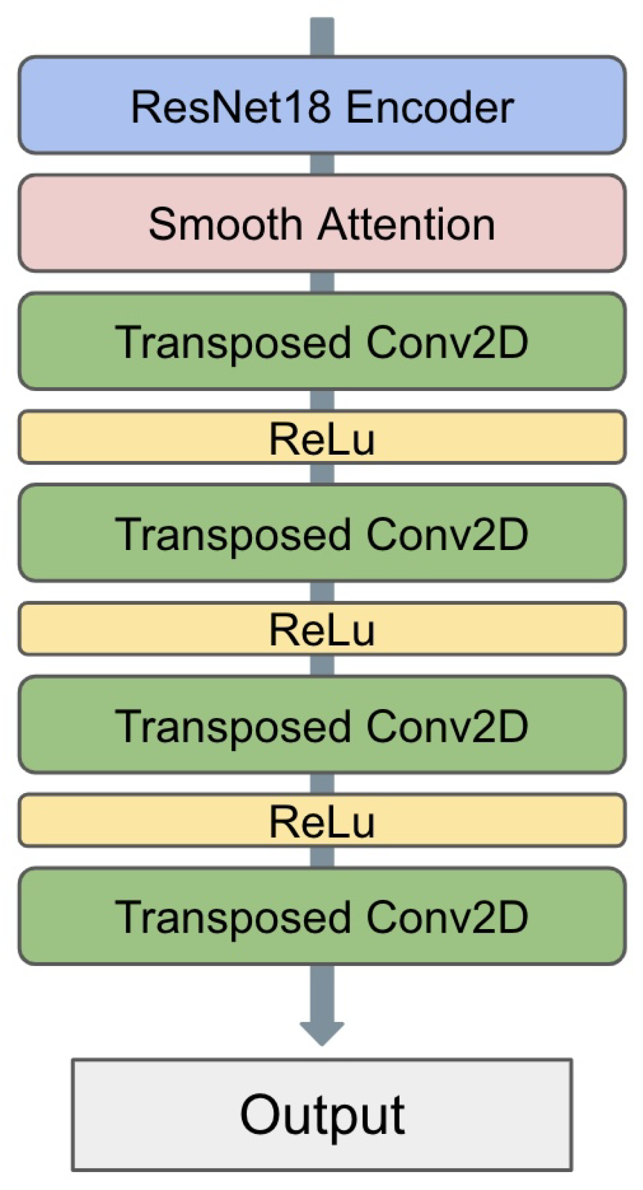
3.1. Architecture Overview
- Query, key, and value projections (3.1.1)
- Attention computation (3.1.2)
- Smoothness enforcement mechanism (3.1.3)
3.1.1. Query, Key, and Value Projections
- Allow the network to learn representations of the input that are suitable for computing attention.
- Enable the module to adjust the channel dimensionality, reducing computational complexity.
- Provide a learned transformation that emphasizes or suppresses aspects of the input for attention computation.
3.1.2. Attention Computation
- represents the matrix multiplication of Q and the transpose of K;
- is the dimensionality of the key vectors;
- is used for scaling to counteract the effect of large dot products in high dimensions;
- Softmax is applied to normalize the attention scores.
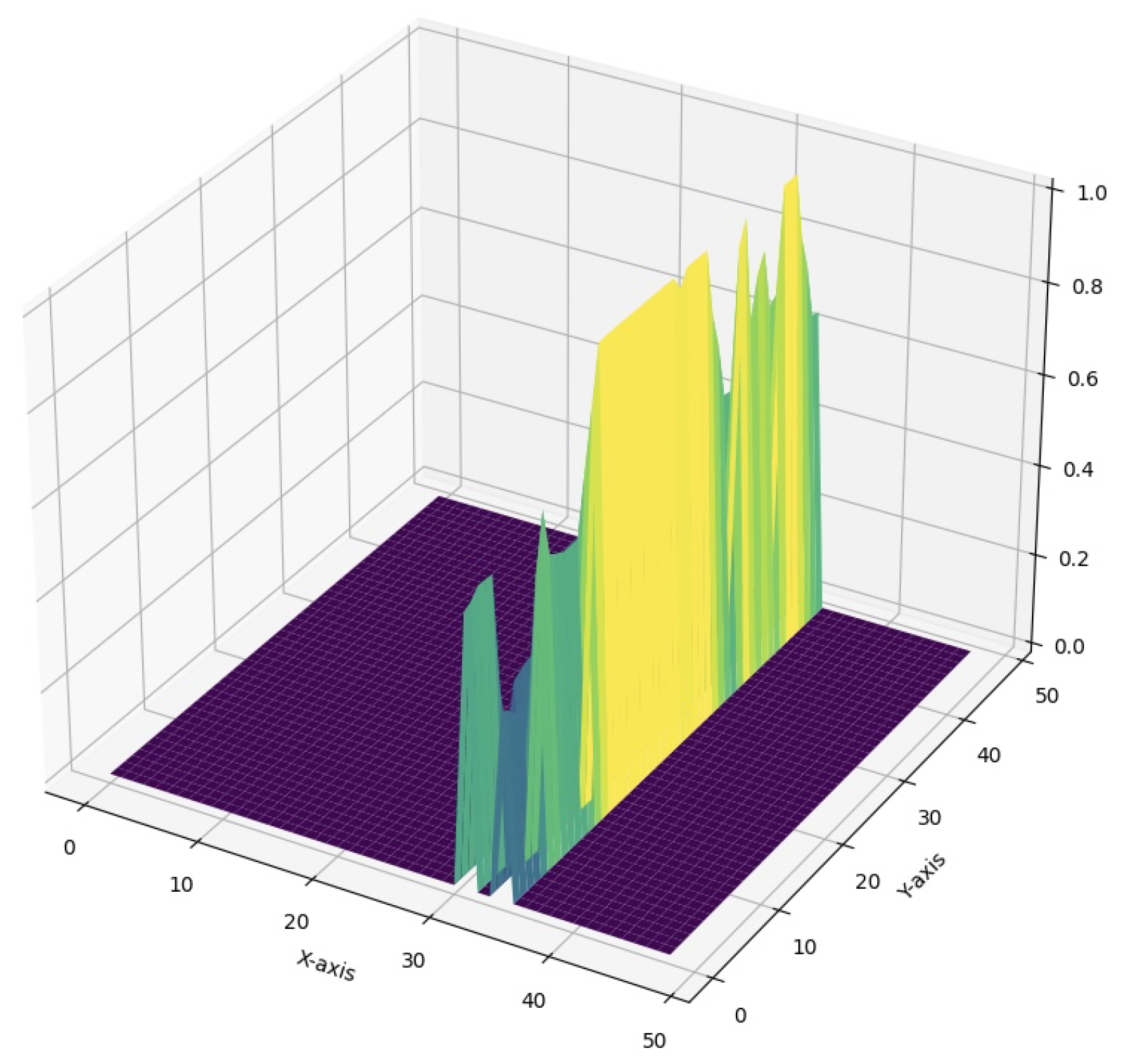
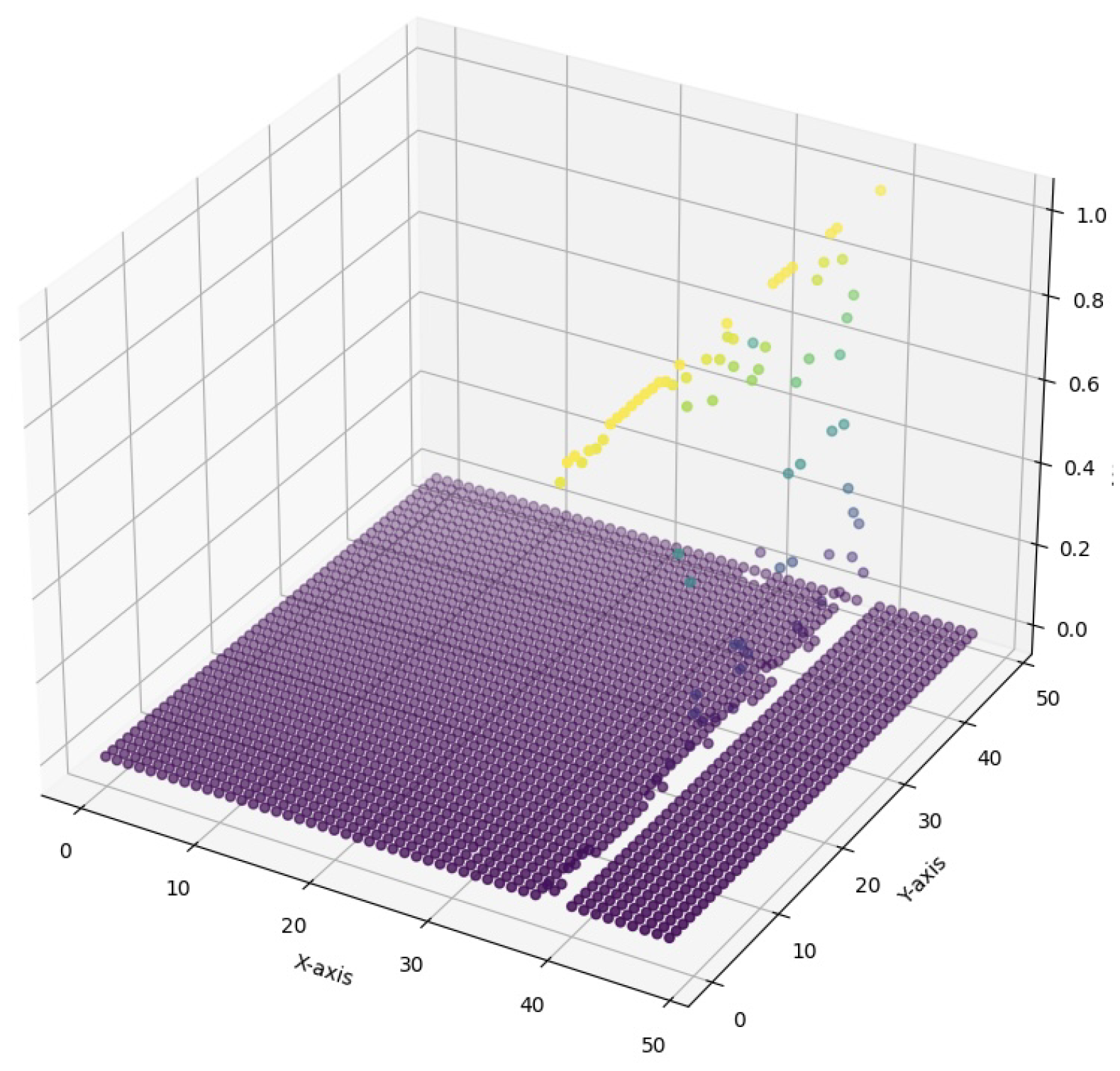
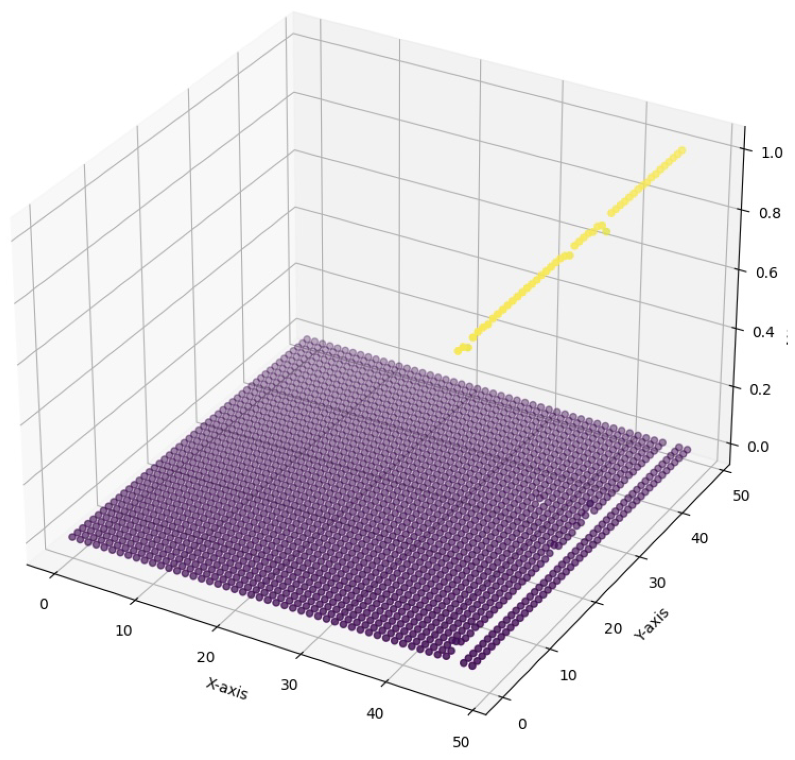
3.1.3. Smoothness Enforcement Mechanism
3.2. Smoothness Thresholding and Mask Creation
3.3. Attention Application with Smoothness Consideration
- is a learnable parameter initialized to zero;
- V is the value projection of the input;
- x is the original input.
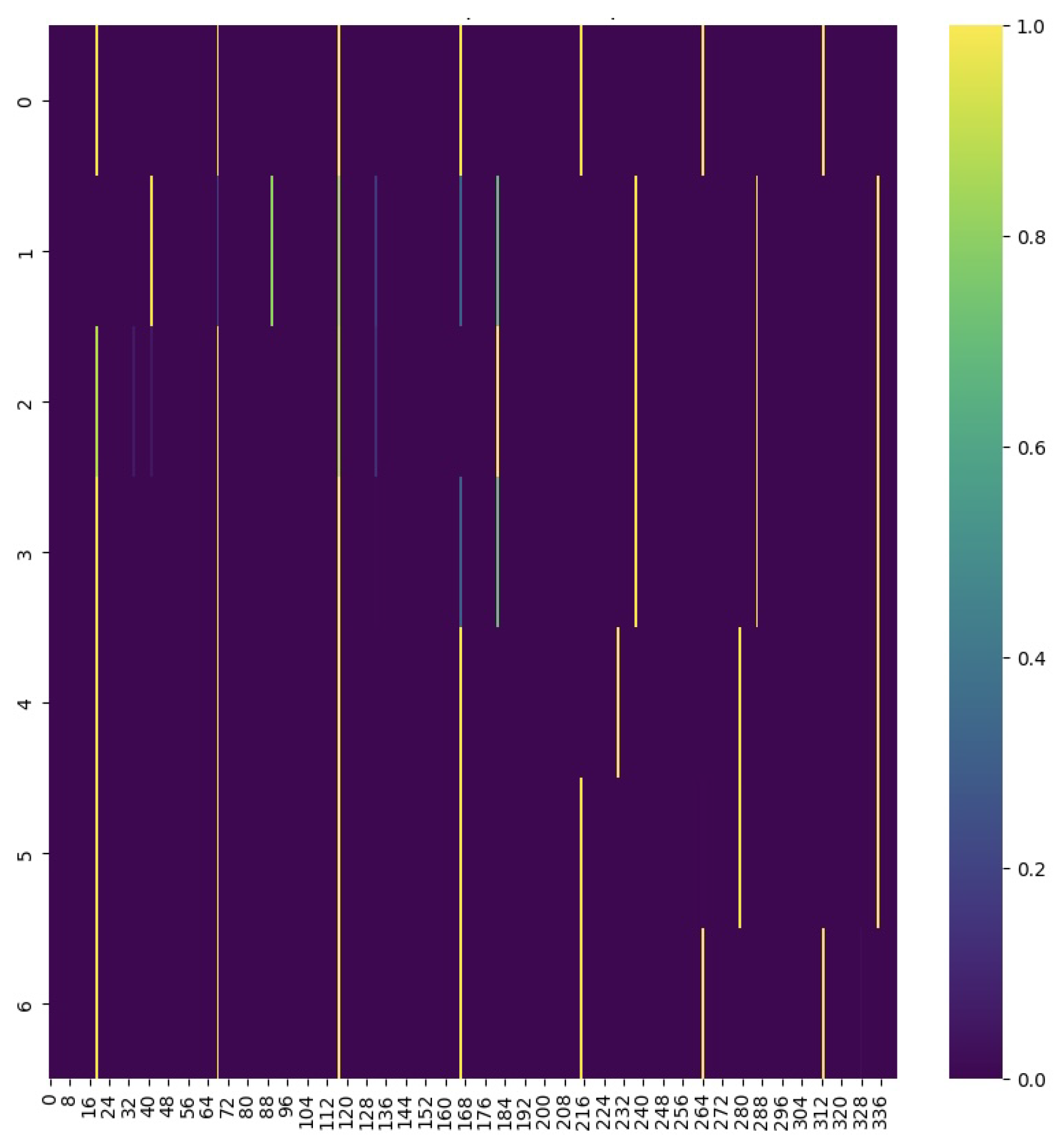
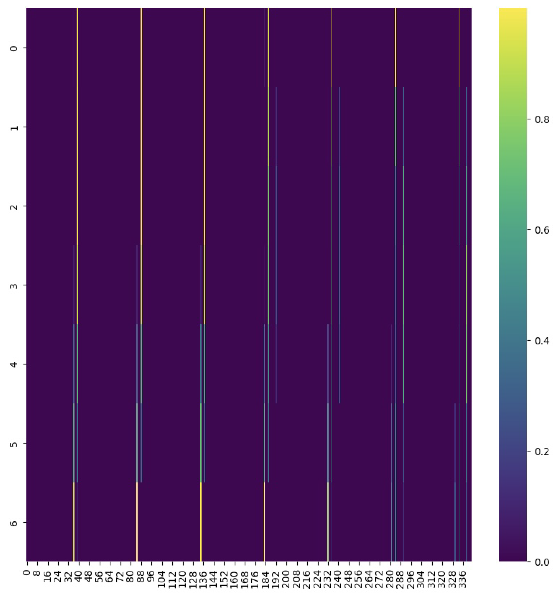
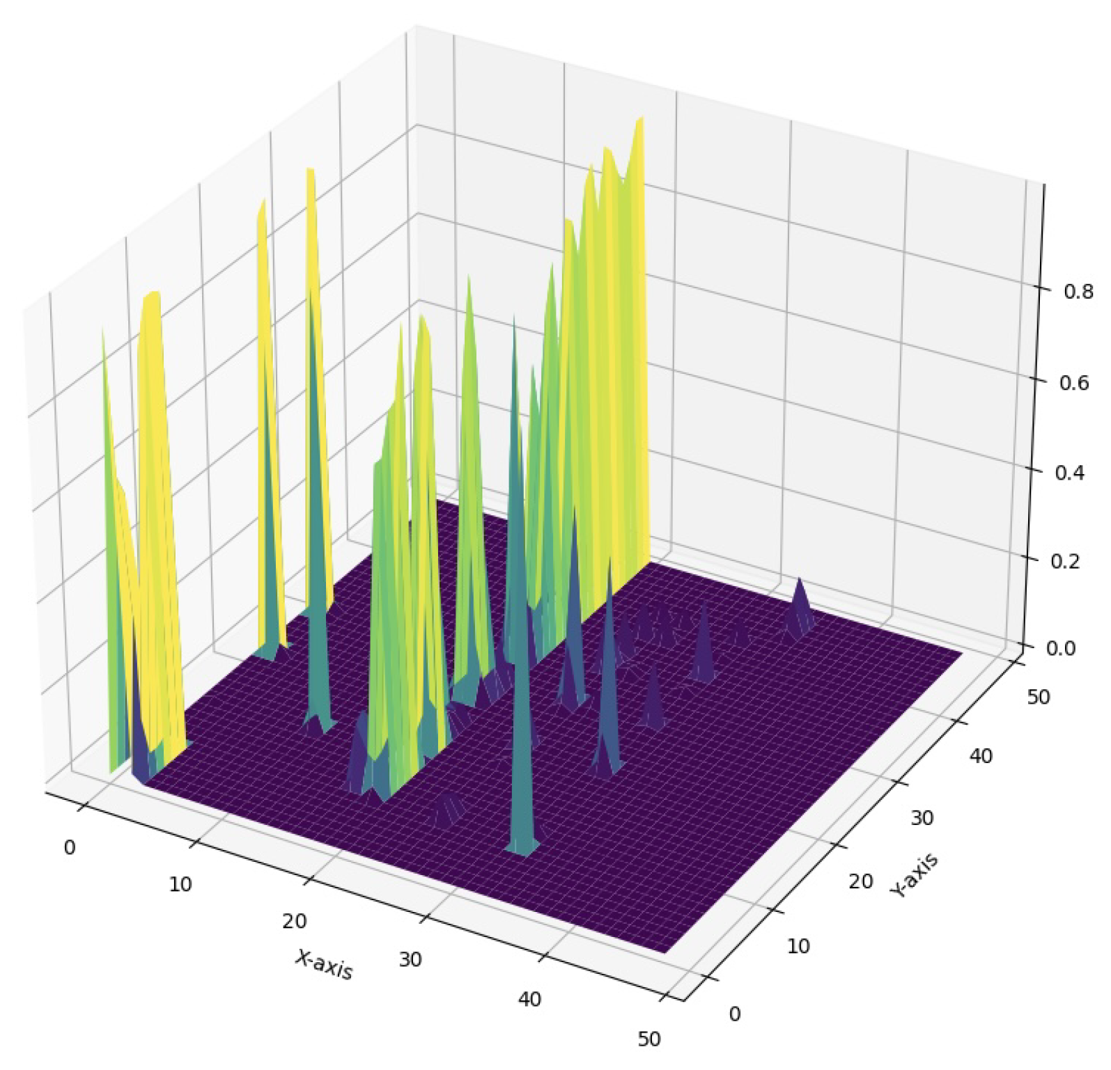
- Spatial Coherence: By enforcing local smoothness, the module encourages the production of more coherent attention maps, improving model’s performance on complex computer vision tasks.
- Noise Reduction: The smoothness constraint acts as a form of regularization, reducing the impact of noise and spurious correlations in the attention computation.
- Interpretability: Smoother attention maps are more interpretable, providing clearer insights into which parts of the input the model is focusing on.
- Adaptive Mechanism: The learnable parameter and the smoothness threshold provide additional level of engineering flexibility, allowing the network to adapt the strength of the smoothness constraint based on the task and data.
4. Experiments
5. Conclusion
Author Contributions
Funding
Data Availability Statement
Acknowledgments
Conflicts of Interest
References
- Vaswani, A. (2017). Attention is all you need. Advances in Neural Information Processing Systems.
- Galassi, A., Lippi, M., & Torroni, P. (2020). Attention in natural language processing. IEEE transactions on neural networks and learning systems, 32(10), 4291-4308. [CrossRef]
- Guo, M. H., Xu, T. X., Liu, J. J., Liu, Z. N., Jiang, P. T., Mu, T. J., ... & Hu, S. M. (2022). Attention mechanisms in computer vision: A survey. Computational visual media, 8(3), 331-368. [CrossRef]
- Yang, X. (2020, December). An overview of the attention mechanisms in computer vision. In Journal of physics: Conference series (Vol. 1693, No. 1, p. 012173). IOP Publishing. [CrossRef]
- Wang, F., & Tax, D. M. (2016). Survey on the attention based RNN model and its applications in computer vision. arXiv preprint arXiv:1601.06823.
- Bello, I., Zoph, B., Vaswani, A., Shlens, J., & Le, Q. V. (2019). Attention augmented convolutional networks. In Proceedings of the IEEE/CVF international conference on computer vision (pp. 3286-3295).
- Ramachandran, P., Parmar, N., Vaswani, A., Bello, I., Levskaya, A., & Shlens, J. (2019). Stand-alone self-attention in vision models. Advances in neural information processing systems, 32.
- Luong, M. T. (2015). Effective approaches to attention-based neural machine translation. arXiv preprint arXiv:1508.04025.
- Zhang, B., Xiong, D., & Su, J. (2018). Neural machine translation with deep attention. IEEE transactions on pattern analysis and machine intelligence, 42(1), 154-163. [CrossRef]
- Maruf, S., Martins, A. F., & Haffari, G. (2019). Selective attention for context-aware neural machine translation. arXiv preprint arXiv:1903.08788.
- You, Q., Jin, H., Wang, Z., Fang, C., & Luo, J. (2016). Image captioning with semantic attention. In Proceedings of the IEEE conference on computer vision and pattern recognition (pp. 4651-4659).
- Sun, J., Jiang, J., & Liu, Y. (2020, December). An introductory survey on attention mechanisms in computer vision problems. In 2020 6th International Conference on Big Data and Information Analytics (BigDIA) (pp. 295-300). IEEE.
- Li, H., Xiong, P., An, J., & Wang, L. (2018). Pyramid attention network for semantic segmentation. arXiv preprint arXiv:1805.10180.
- Guo, M. H., Lu, C. Z., Hou, Q., Liu, Z., Cheng, M. M., & Hu, S. M. (2022). Segnext: Rethinking convolutional attention design for semantic segmentation. Advances in Neural Information Processing Systems, 35, 1140-1156.
- Konate, S., Lebrat, L., Santa Cruz, R., Bourgeat, P., Dorê, V., Fripp, J., ... & Salvado, O. (2021, April). Smocam: Smooth conditional attention mask for 3d-regression models. In 2021 IEEE 18th International Symposium on Biomedical Imaging (ISBI) (pp. 362-366). IEEE.
- Yao, Y., Ren, J., Xie, X., Liu, W., Liu, Y. J., & Wang, J. (2019). Attention-aware multi-stroke style transfer. In Proceedings of the IEEE/CVF conference on computer vision and pattern recognition (pp. 1467-1475).
- Jiang, P. T., Han, L. H., Hou, Q., Cheng, M. M., & Wei, Y. (2021). Online attention accumulation for weakly supervised semantic segmentation. IEEE Transactions on Pattern Analysis and Machine Intelligence, 44(10), 7062-7077. [CrossRef]
- Alexey, D. (2020). An image is worth 16x16 words: Transformers for image recognition at scale. arXiv preprint arXiv: 2010.11929.
- Liu, Z., Lin, Y., Cao, Y., Hu, H., Wei, Y., Zhang, Z., ... & Guo, B. (2021). Swin transformer: Hierarchical vision transformer using shifted windows. In Proceedings of the IEEE/CVF international conference on computer vision (pp. 10012-10022).
- Wang, X., Girshick, R., Gupta, A., & He, K. (2018). Non-local neural networks. In Proceedings of the IEEE conference on computer vision and pattern recognition (pp. 7794-7803).
- Woo, S., Park, J., Lee, J. Y., & Kweon, I. S. (2018). Cbam: Convolutional block attention module. In Proceedings of the European conference on computer vision (ECCV) (pp. 3-19).
- Zheng, S., Jayasumana, S., Romera-Paredes, B., Vineet, V., Su, Z., Du, D., ... & Torr, P. H. (2015). Conditional random fields as recurrent neural networks. In Proceedings of the IEEE international conference on computer vision (pp. 1529-1537).
- Isola, P., Zhu, J. Y., Zhou, T., & Efros, A. A. (2017). Image-to-image translation with conditional adversarial networks. In Proceedings of the IEEE conference on computer vision and pattern recognition (pp. 1125-1134).
- Graves, A. (2016). Adaptive computation time for recurrent neural networks. arXiv preprint arXiv:1603.08983.
- Bello, I., Zoph, B., Vaswani, A., Shlens, J., & Le, Q. V. (2019). Attention augmented convolutional networks. In Proceedings of the IEEE/CVF international conference on computer vision (pp. 3286-3295).
- Yang, J., Li, C., Zhang, P., Dai, X., Xiao, B., Yuan, L., & Gao, J. (2021). Focal self-attention for local-global interactions in vision transformers. arXiv preprint arXiv:2107.00641.
- Wang, J., Chen, Y., Hao, S., Peng, X., & Hu, L. (2019). Deep learning for sensor-based activity recognition: A survey. Pattern recognition letters, 119, 3-11. [CrossRef]
- Liu, R., Lehman, J., Molino, P., Petroski Such, F., Frank, E., Sergeev, A., & Yosinski, J. (2018). An intriguing failing of convolutional neural networks and the coordconv solution. Advances in neural information processing systems, 31.
- Choromanski, K., Likhosherstov, V., Dohan, D., Song, X., Gane, A., Sarlos, T., ... & Weller, A. (2020). Rethinking attention with performers. arXiv preprint arXiv:2009.14794.
- Solomon, J., Crane, K., Butscher, A., & Wojtan, C. (2014). A general framework for bilateral and mean shift filtering. arXiv preprint arXiv:1405.4734, 1(2), 3.
- Wang, J., & Hu, X. (2021). Convolutional neural networks with gated recurrent connections. IEEE Transactions on Pattern Analysis and Machine Intelligence, 44(7), 3421-3435. [CrossRef]
- Volz, S., Bruhn, A., Valgaerts, L., & Zimmer, H. (2011, November). Modeling temporal coherence for optical flow. In 2011 International Conference on Computer Vision (pp. 1116-1123). IEEE.
- Tong, X., Xu, R., Liu, K., Zhao, L., Zhu, W., & Zhao, D. (2023). A Deep-Learning Approach for Low-Spatial-Coherence Imaging in Computer-Generated Holography. Advanced Photonics Research, 4(1), 2200264. [CrossRef]
- Zabih, R., & Kolmogorov, V. (2004, June). Spatially coherent clustering using graph cuts. In Proceedings of the 2004 IEEE Computer Society Conference on Computer Vision and Pattern Recognition, 2004. CVPR 2004. (Vol. 2, pp. II-II). IEEE.
- Li, F., Lebanon, G., & Sminchisescu, C. (2012, June). Chebyshev approximations to the histogram χ2 kernel. In 2012 IEEE Conference on Computer Vision and Pattern Recognition (pp. 2424-2431). IEEE.
- Koenderink, J., & van Doom, A. (1998). Shape from Chebyshev nets. In Computer Vision—ECCV’98: 5th European Conference on Computer Vision Freiburg, Germany, June 2–6, 1998 Proceedings, Volume II 5 (pp. 215-225). Springer Berlin Heidelberg.
- Wah, C., Branson, S., Welinder, P., Perona, P., & Belongie, S. (2011). The caltech-ucsd birds-200-2011 dataset.
- Ulucan, O., Karakaya, D., & Turkan, M. (2020, October). A large-scale dataset for fish segmentation and classification. In 2020 Innovations in Intelligent Systems and Applications Conference (ASYU) (pp. 1-5). IEEE.
- DiversisAI. (n.d.). Fire segmentation image dataset. Kaggle. https://www.kaggle.com/datasets/diversisai/fire-segmentation-image-dataset.
- Jha, D., Ali, S., Emanuelsen, K., Hicks, S. A., Thambawita, V., Garcia-Ceja, E., Riegler, M. A., de Lange, T., Schmidt, P. T., Johansen, H. D., Johansen, D., & Halvorsen, P. (2021). Kvasir-Instrument: Diagnostic and therapeutic tool segmentation dataset in gastrointestinal endoscopy. In MultiMedia Modeling (pp. 218–229). Springer International Publishing.
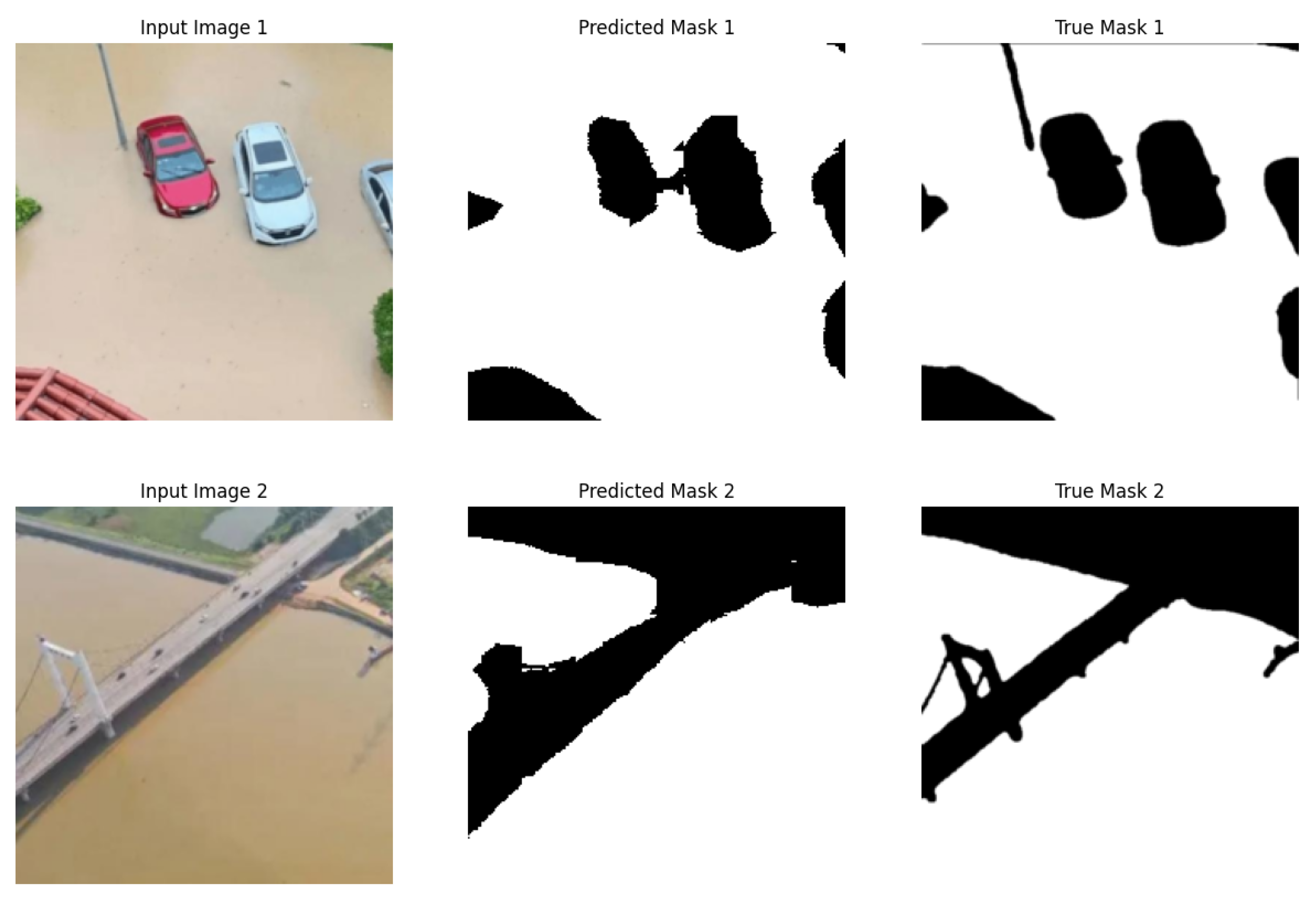
- Li, H. (n.d.). Flood semantic segmentation dataset. Kaggle. https://www.kaggle.com/datasets/lihuayang111265/flood-semantic-segmentation-dataset.
- Siddique, N., Paheding, S., Elkin, C. P., & Devabhaktuni, V. (2021). U-net and its variants for medical image segmentation: A review of theory and applications. IEEE access, 9, 82031-82057. [CrossRef]
- Ronneberger, O., Fischer, P., & Brox, T. (2015). U-net: Convolutional networks for biomedical image segmentation. In Medical image computing and computer-assisted intervention–MICCAI 2015: 18th international conference, Munich, Germany, October 5-9, 2015, proceedings, part III 18 (pp. 234-241). Springer International Publishing.
- Oktay, O., Schlemper, J., Folgoc, L. L., Lee, M., Heinrich, M., Misawa, K., ... & Rueckert, D. (2018). Attention u-net: Learning where to look for the pancreas. arXiv preprint arXiv:1804.03999.
- He, K., Zhang, X., Ren, S., & Sun, J. (2016). Deep residual learning for image recognition. In Proceedings of the IEEE conference on computer vision and pattern recognition (pp. 770-778).
- Gao, H., Yuan, H., Wang, Z., & Ji, S. (2019). Pixel transposed convolutional networks. IEEE transactions on pattern analysis and machine intelligence, 42(5), 1218-1227. [CrossRef]
- Cho, K., Courville, A., & Bengio, Y. (2015). Describing multimedia content using attention-based encoder-decoder networks. IEEE Transactions on Multimedia, 17(11), 1875-1886. [CrossRef]
- Ji, Z., Xiong, K., Pang, Y., & Li, X. (2019). Video summarization with attention-based encoder–decoder networks. IEEE Transactions on Circuits and Systems for Video Technology, 30(6), 1709-1717. [CrossRef]
- Garcia-Garcia, A., Orts-Escolano, S., Oprea, S., Villena-Martinez, V., & Garcia-Rodriguez, J. (2017). A review on deep learning techniques applied to semantic segmentation. arXiv preprint arXiv:1704.06857.
- Du, S., Fan, H., Zhao, M., Zong, H., Hu, J., & Li, P. (2022). A two-stage method for single image de-raining based on attention smoothed dilated network. IET Image Processing, 16(10), 2557-2567. [CrossRef]
- Ouyang, W., Zeng, X., & Wang, X. (2013). Modeling mutual visibility relationship in pedestrian detection. In Proceedings of the IEEE conference on computer vision and pattern recognition (pp. 3222-3229).
| Metric | Test IOU | Test Dice | Test Acc | Test Prec | Test Recall | Test F1 |
|---|---|---|---|---|---|---|
| 0.1 | 0.7933 | 0.9231 | 0.9686 | 0.7674 | 0.9838 | 0.8550 |
| 0.2 | 0.8028 | 0.9294 | 0.9670 | 0.7457 | 0.9829 | 0.8430 |
| 0.3 | 0.7997 | 0.9292 | 0.9672 | 0.7641 | 0.9829 | 0.8521 |
| 0.4 | 0.7894 | 0.9186 | 0.9679 | 0.7654 | 0.9799 | 0.8495 |
| 0.5 | 0.7963 | 0.9258 | 0.9672 | 0.7609 | 0.9827 | 0.8494 |
| 0.6 | 0.7949 | 0.9260 | 0.9693 | 0.7740 | 0.9812 | 0.8562 |
| 0.7 | 0.7952 | 0.9239 | 0.9677 | 0.7685 | 0.9811 | 0.8526 |
| 0.8 | 0.8003 | 0.9272 | 0.9678 | 0.7700 | 0.9808 | 0.8493 |
| 0.9 | 0.7994 | 0.9229 | 0.9699 | 0.7881 | 0.9823 | 0.8610 |
| 2.0 | 0.7909 | 0.9222 | 0.9667 | 0.7497 | 0.9827 | 0.8453 |
| Metric | Test IOU | Test Dice | Test Acc | Test Prec | Test Recall | Test F1 |
|---|---|---|---|---|---|---|
| 0.1 | 0.9344 | 0.9764 | 0.9882 | 0.9426 | 0.9904 | 0.9618 |
| 0.2 | 0.9364 | 0.9784 | 0.9887 | 0.9434 | 0.9916 | 0.9638 |
| 0.3 | 0.9309 | 0.9749 | 0.9879 | 0.9493 | 0.9901 | 0.9600 |
| 0.4 | 0.9320 | 0.9751 | 0.9883 | 0.9399 | 0.9898 | 0.9627 |
| 0.5 | 0.9355 | 0.9787 | 0.9886 | 0.9426 | 0.9910 | 0.9630 |
| 0.6 | 0.9283 | 0.9706 | 0.9874 | 0.9383 | 0.9872 | 0.9602 |
| 0.7 | 0.9247 | 0.9694 | 0.9886 | 0.9519 | 0.9866 | 0.9620 |
| 0.8 | 0.9290 | 0.9731 | 0.9885 | 0.9434 | 0.9882 | 0.9626 |
| 0.9 | 0.9336 | 0.9759 | 0.9879 | 0.9465 | 0.9899 | 0.9612 |
| 2.0 | 0.9363 | 0.9781 | 0.9886 | 0.9436 | 0.9915 | 0.9611 |
| Metric | Test IOU | Test Dice | Test Acc | Test Prec | Test Recall | Test F1 |
|---|---|---|---|---|---|---|
| 0.1 | 0.8484 | 0.9228 | 0.9904 | 0.4903 | 0.9630 | 0.6322 |
| 0.2 | 0.8512 | 0.9246 | 0.9913 | 0.4868 | 0.9633 | 0.6403 |
| 0.3 | 0.8488 | 0.9189 | 0.9925 | 0.5269 | 0.9599 | 0.6377 |
| 0.4 | 0.8518 | 0.9277 | 0.9914 | 0.4907 | 0.9662 | 0.6446 |
| 0.5 | 0.8501 | 0.9248 | 0.9910 | 0.4753 | 0.9648 | 0.6329 |
| 0.6 | 0.8507 | 0.9268 | 0.9919 | 0.5096 | 0.9656 | 0.6489 |
| 0.7 | 0.8498 | 0.9231 | 0.9918 | 0.5027 | 0.9628 | 0.6460 |
| 0.8 | 0.8480 | 0.9208 | 0.9918 | 0.5057 | 0.9594 | 0.6520 |
| 0.9 | 0.8497 | 0.9231 | 0.9915 | 0.4888 | 0.9608 | 0.6314 |
| 2.0 | 0.8504 | 0.9211 | 0.9911 | 0.4837 | 0.9623 | 0.6399 |
| Metric | Test IOU | Test Dice | Test Acc | Test Prec | Test Recall | Test F1 |
|---|---|---|---|---|---|---|
| 0.1 | 0.9105 | 0.9405 | 0.9853 | 0.9427 | 0.9370 | 0.9138 |
| 0.2 | 0.9248 | 0.9536 | 0.9881 | 0.9489 | 0.9674 | 0.9294 |
| 0.3 | 0.9223 | 0.9504 | 0.9876 | 0.9632 | 0.9548 | 0.9263 |
| 0.4 | 0.9071 | 0.9348 | 0.9852 | 0.9231 | 0.9367 | 0.9136 |
| 0.5 | 0.9125 | 0.9420 | 0.9848 | 0.9162 | 0.9364 | 0.9163 |
| 0.6 | 0.9054 | 0.9371 | 0.9847 | 0.9077 | 0.9326 | 0.9167 |
| 0.7 | 0.9052 | 0.9374 | 0.9828 | 0.9121 | 0.9345 | 0.9081 |
| 0.8 | 0.9093 | 0.9394 | 0.9861 | 0.9083 | 0.9587 | 0.9217 |
| 0.9 | 0.9091 | 0.9390 | 0.9857 | 0.9115 | 0.9470 | 0.9197 |
| 2.0 | 0.9108 | 0.9376 | 0.9855 | 0.9152 | 0.9479 | 0.9208 |
| Metric | Test IOU | Test Dice | Test Acc | Test Prec | Test Recall | Test F1 |
|---|---|---|---|---|---|---|
| 0.1 | 0.8746 | 0.9321 | 0.9571 | 0.9450 | 0.9669 | 0.9515 |
| 0.2 | 0.8694 | 0.9274 | 0.9542 | 0.9521 | 0.9790 | 0.9486 |
| 0.3 | 0.8765 | 0.9309 | 0.9543 | 0.9432 | 0.9712 | 0.9480 |
| 0.4 | 0.8772 | 0.9334 | 0.9554 | 0.9595 | 0.9662 | 0.9501 |
| 0.5 | 0.8374 | 0.9309 | 0.9560 | 0.9556 | 0.9691 | 0.9495 |
| 0.6 | 0.8728 | 0.9294 | 0.9531 | 0.9501 | 0.9658 | 0.9470 |
| 0.7 | 0.8744 | 0.9317 | 0.9555 | 0.9452 | 0.9612 | 0.9502 |
| 0.8 | 0.8674 | 0.9263 | 0.9522 | 0.9419 | 0.9622 | 0.9446 |
| 0.9 | 0.8696 | 0.9292 | 0.9518 | 0.9517 | 0.9646 | 0.9469 |
| 2.0 | 0.8720 | 0.9308 | 0.9542 | 0.9514 | 0.9605 | 0.9468 |
Disclaimer/Publisher’s Note: The statements, opinions and data contained in all publications are solely those of the individual author(s) and contributor(s) and not of MDPI and/or the editor(s). MDPI and/or the editor(s) disclaim responsibility for any injury to people or property resulting from any ideas, methods, instructions or products referred to in the content. |
© 2024 by the authors. Licensee MDPI, Basel, Switzerland. This article is an open access article distributed under the terms and conditions of the Creative Commons Attribution (CC BY) license (http://creativecommons.org/licenses/by/4.0/).


