Comparison of Different Quantitative Precipitation Estimation Methods Based on a Severe Rainfall Event in Tuscany, Italy, November 2023

Accurate Quantitative Precipitation Estimation (QPE) is fundamental for a large number of hydrometeorological applications, especially when addressing extreme rainfall phenomena. This paper presents a comprehensive comparison of various rainfall estimation methods, specifically those relying on weather radar data, rain gauge data, and their fusion. The study evaluates the accuracy and reliability of each method in estimating rainfall for a severe event that occurred in Tuscany, Italy. The obtained results indicate that merging radar and rain gauge data outperform both individual approaches by reducing errors and improving the overall reliability of precipitation estimates. The study highlights the importance of data fusion in enhancing the accuracy of QPE and also supports its application in operational contexts, providing evidence for the greater reliability of merging methods

Keywords:

Subject: Environmental and Earth Sciences - Remote Sensing

1. Introduction

Quantitative precipitation estimation (QPE) is a critical element in meteorology and hydrology, making accurate QPE methods essential for numerous applications, including flood forecasting. QPE methods typically employ data from two types of instrument: rain gauges and weather radars. Given the specific advantages and limitations of each of them, the information about rainfall provided by these instruments are somehow complementary. Therefore, their combination represents a solid ground for achieving accurate precipitation estimation.

Rain gauges measure precipitation directly, providing highly accurate data on the amount of rainfall at a specific locations. Given their precision, these instruments are used for calibrating and validating other precipitation estimation methods. However, rain gauge measurements may be affected by errors, both systematic and random, depending on the atmospheric conditions and the type of rain gauge [1,2]. Taking into account the point-wise nature of rain gauges, the rainfall measurements need to be spatially interpolated in order to generate a 2D rainfall map; for this purpose, deterministic (e.g., inverse distance weighting [3]) or geostatistical (e.g., kriging [4]) techniques are typically used (see [5,6] for a comparison). The nature of these instruments represents also their main limitation: in fact, a dense gauges network is required to capture the spatial variability of the rainfall patterns, especially in case of severe small-scale phenomena.

Weather radars, on the contrary, can monitor precipitation over large areas with high temporal and spatial resolution. Radars emit microwave pulses and measure the power backscattered from ensemble of hydrometeors, providing a practically continuous monitoring of the spatial distribution of rainfall an of its intensity [7]. Despite their broad coverage and excellent resolution, both in time and space, radar-based QPE is subject to several sources of error, including signal attenuation due to rainfall itself, ground clutter and beam blockage [8]. Moreover, radars do not provide direct rainfall measures, thus a conversion is required to obtain the QPE. This conversion is typically made resorting to the so-called Z–R relationship [9]:

Z = a R^{b},

(1)

which relates the reflectivity factor Z (expressed in

{mm}^{6} \cdot

m^{- 3}

), a parameter derived from the backscattered power measured by the radar, and the rainfall rate R (expressed in mm·

h^{- 1}

). Unfortunately, the choice of the coefficients a and b is critical. In fact, both Z and R depend on the drop size distribution (DSD), which is influenced by the type of event, the geographical area and the climatic conditions [8,10,11]. As a result, a and b are highly variable [12], and using the Z-R relation with a priori-fixed coefficients can lead to significant rainfall estimation errors [13].

Due to the complementary features and issues of rain gauges and weather radars, integrating their data can be usefully exploited to mitigate their limitations and to enhance the QPE accuracy. For this reason, merging rain gauge and radar data has been investigated for several years and various methods, with different approaches, have been developed (see for instance the review in [14]). One criterion with which the different approaches can be categorized is based on how the two data types are employed during the fusion procedure [14]. Methods belonging to the geostatistical interpolation category use the rainfall point measurements provided by rain gauges as primary quantitative information source, and the radar rainfall field as auxiliary spatial information to improve the accuracy of the estimation. These methods derive mostly from the kriging technique and the most employed is the kriging with external drift (KED), in which the external auxiliary variable (i.e, the radar-based QPE) is incorporated in the interpolation process of the primary variable (i.e., rainfall data provided by rain gauges) [4]. This category includes also the conditional merging (CM), in which the kriging-based QPE is corrected by adding an error obtained from radar rainfall observations [15]. Different merging approaches consist in adjusting the radar-based QPE by exploiting the rain gauge measurements. In this kind of methods – typically called radar bias adjustment methods because they address the issue of systematic bias in radar data – a multiplicative or additive correction factor obtained by comparing radar estimates with rain gauge measures is applied to the radar rainfall field. The simplest method in this category is the mean field bias (MFB) adjustment, in which a spatially constant multiplicative correction factor is used [9]. Other adjustment methods, such as that proposed by Brandes (Brandes spatial adjustment, BSA) [16], consider a correction factor that varies in space, so as to take into account of nonuniform bias across the radar coverage area. Finally, merging methods employing a space-time varying Z–R relationship have been proposed, such as that presented in [17] that is based on the dynamic adaptation of the coefficients a and b. This method, named space-time adaptive coefficient conversion (STACC), has proven its effectiveness for QPE especially when rainfall events with localized intense peaks affect areas characterized by a sparse rain gauge network [18].

In this study, we present an evaluation of different QPE methods based on data collected during a severe rainfall event in Tuscany, Italy. Methods relying solely on rain gauge data, solely on radar data, and on their integration, are considered. The paper is structured as follows: in Section 2, we first describe the event examined in this study and the employed radar and rain gauge datasets; then, we present the different QPE methods considered, as well as the procedure adopted to evaluate and compare them. The experimental results are shown and discussed in Section 3. Finally, in Section 4, we draw some concluding remarks.

2. Materials and Methods

2.1. Meteorological Event Description

The information that follows, concerning the meteorological phenomenon considered in this study, comes from the meteorological report provided by the LaMMA (Environmental Modeling and Monitoring Laboratory for Sustainable Development) Consortium [19], to which the reader is referred for further details.

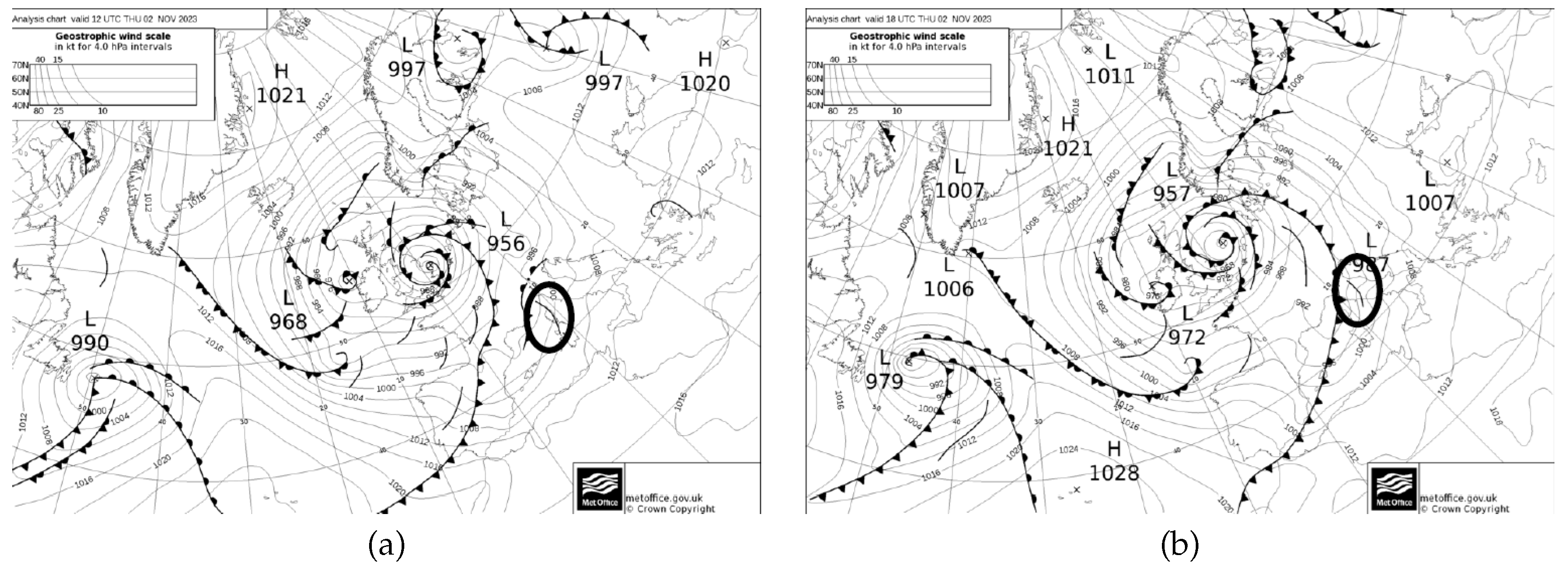
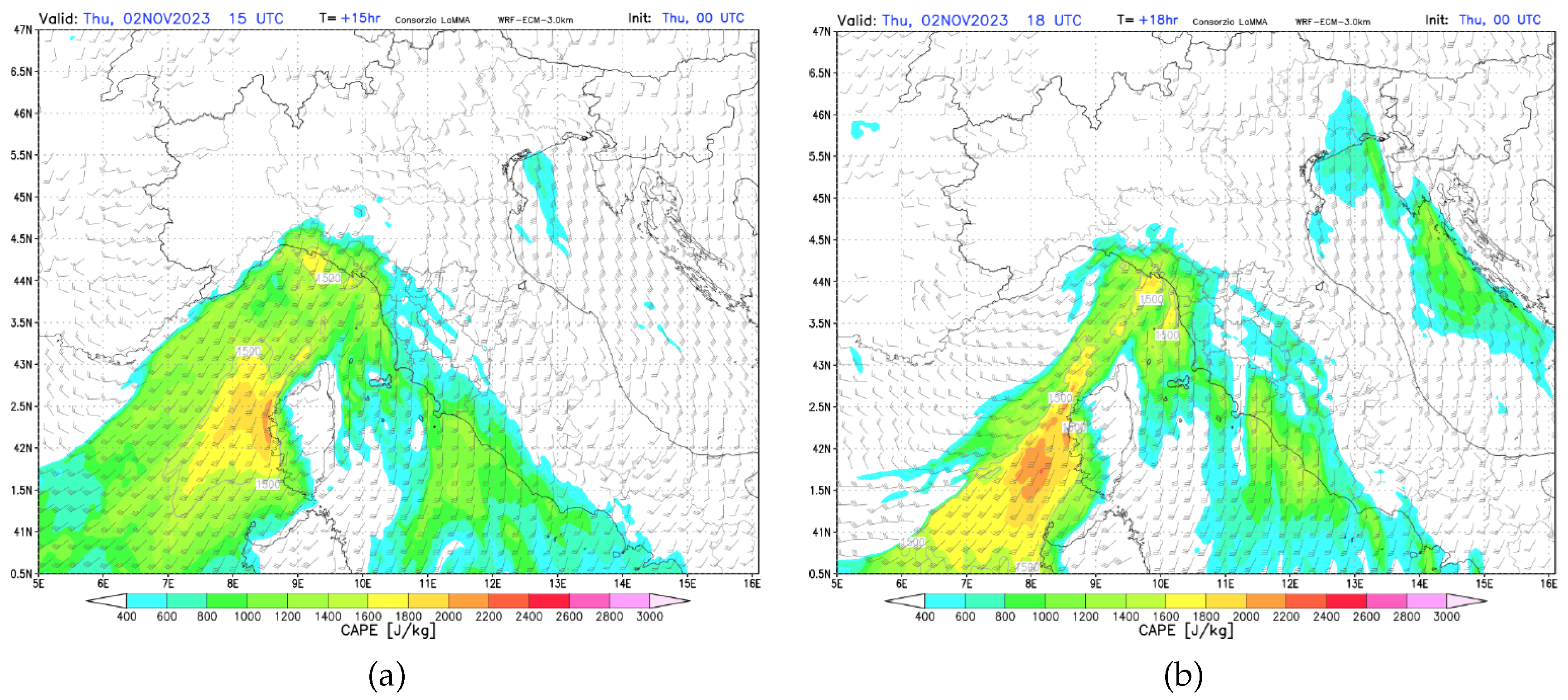
In the afternoon of November 2, 2023, in Tuscany, the movement of a relatively stationary instability line (Figure 1) ahead of a cold front facilitated the development of several thunderstorms. These storms were intensified by an energetically favorable atmosphere (Figure 2) and highly humid low-level conditions, leading to an intense localized precipitation. Specifically, starting at 15:30 UTC, the convergence of strong winds in the southern parts of the region with the gradual influx of winds affecting the northern parts, combined with the advance of cooler air aloft and favorable conditions in the lower levels, led to the formation of a thunderstorm line. This system remained nearly stationary until 20:30 UTC, extending from the provinces of Livorno and Pisa to the provinces of Pistoia, Prato, and Florence. The location, intensity, and stationary nature of this thunderstorm system exhibited nonlinear characteristics and presented significant forecasting challenges. As a result of the heavy precipitation, some rivers and creeks flooded, causing extensive damages to the environment and affecting local communities.

2.2. Datasets

2.2.1. Radar Dataset

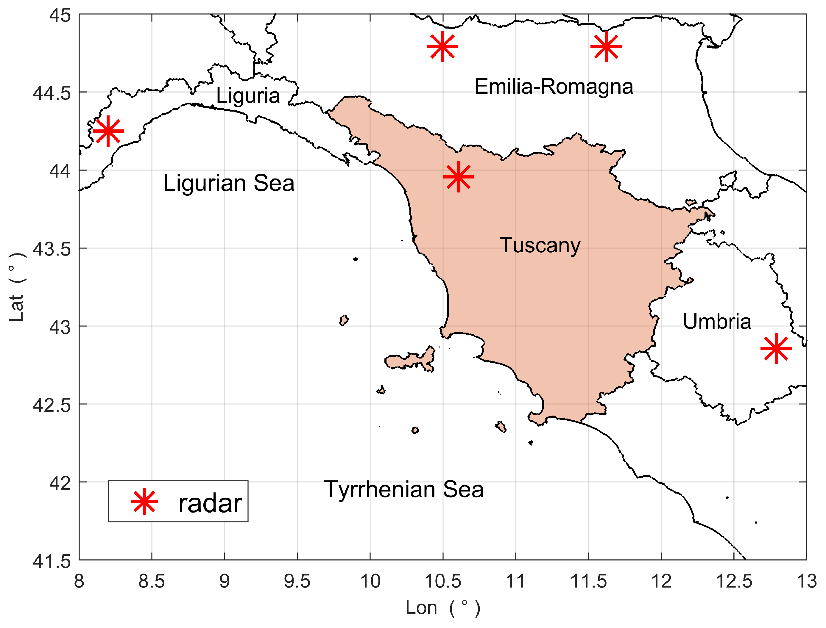
The weather radar data used in this study were collected by the Italian National weather radar network. Managed by the Italian National Civil Protection Department (DPCN), the network consists of 26 radar systems (22 C-band radars and 4 X-band radars, most of them dual-polarized) distributed to cover the entire national territory. Figure 3 shows the radar systems of the network that cover Tuscany. Specifically, these systems are C-band dual-polarized radars located in Monte Crocione (Tuscany, lat:

{43.96}^{\circ}

, lon:

{10.61}^{\circ}

, height: 1017 m a.s.l.), Monte Settepani (Liguria, lat:

{44.25}^{\circ}

, lon:

{8.20}^{\circ}

, height: 1390 m a.s.l.), Gattatico (Emilia Romagna, lat:

{44.79}^{\circ}

, lon:

{10.50}^{\circ}

, height: 34 m a.s.l.), San Pietro Capofiume (Emilia Romagna, lat:

{44.66}^{\circ}

, lon:

{11.62}^{\circ}

, height: 10 m a.s.l.), and Monte Serano (Umbria, lat:

{42.86}^{\circ}

, lon:

{12.79}^{\circ}

, height: 1428 m a.s.l.).

The radars of the network perform synchronous scans every 5 minutes. The raw data from all systems are processed by the DPCN (procedures are described in [20]), which afterward provides national-scale composite products. The radar reflectivity composite products include Constant Altitude Plan Position Indicator (CAPPI) – namely, the reflectivity at a specific altitude (from 1000 m up to 7000 m) obtained by interpolating data from scans made at multiple elevation angles – and Vertical Maximum Intensity (VMI), that is the maximum reflectivity value detected vertically above each ground pixel.

When facing the problem of merging radar and rain gauge data for QPE, the height of radar observations must be carefully considered, as it has an impact on estimation accuracy. In fact, several factors are involved in the choice of the most appropriate height for the reflectivity product, including local orography and topography, which may cause beam blockage and ground clutter, as well as vertical variations in precipitation resulting from evaporation, wind shear, and changes in hydrometeor type [8]. Considering the specific situation of Tuscany, we utilized the CAPPI radar reflectivity at an altitude of 2000 m to balance the various issues and reach a good compromise. 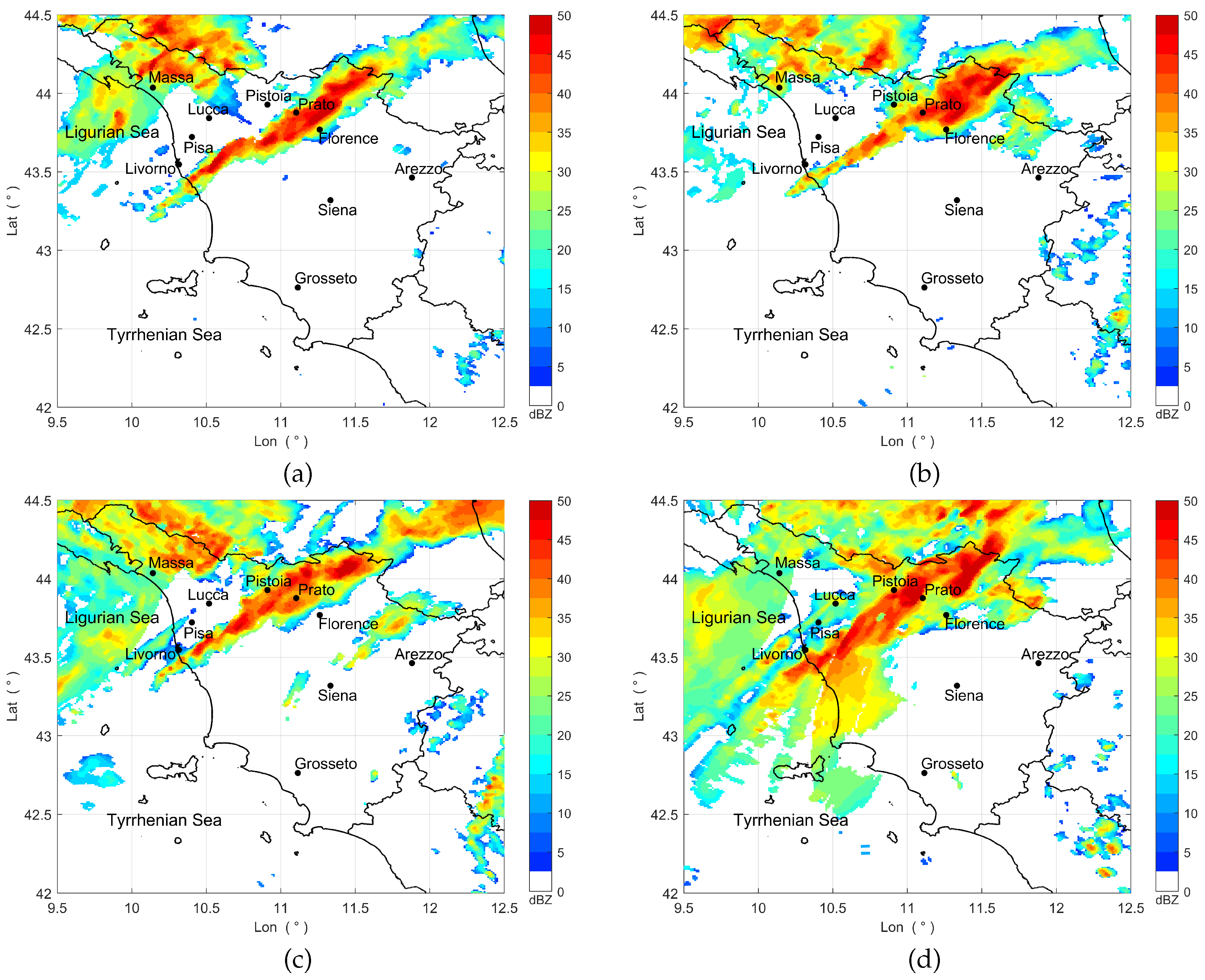Figure 4 shows the chosen product, which is available with a time step of 10 minutes on November 2, 2023. The 2D maps of reflectivity Z have a spatial resolution of 1×1

{km}^{2}

(when mapped onto the x-y Cartesian coordinate system).

2.2.2. Rain Gauge Dataset

In this study, we used rainfall data from the rain gauge network of Tuscany, which is illustrated in Figure 5. The network is composed of 425 tipping-bucket rain gauges located across the entire 22,987

{km}^{2}

area of Tuscany, which means approximately one gauge every 54

{km}^{2}

. Near real-time measurements of accumulated rainfall at 15-minute intervals, recorded by all available stations, are made accessible online through a dedicated platform [21].

By means of the rain gauge data, we defined the “study area” through the following procedure. First, we selected the time interval from 15:30 UTC to 20:30 UTC (i.e., when the considered rainfall event was most intense). Next, we calculated the convex hull encompassing all rain gauges that recorded an average rainfall rate of at least 1 mm·

h^{- 1}

during that interval. The study area was then defined as the region enclosed by the convex hull also shown in Figure 5.

2.3. QPE Methods

2.3.1. Radar-Based Method

Estimating rainfall by using solely weather radar data is typically done through the empirical relationship expressed in (1). In this work, we computed the rainfall field (in mm) as follows: first, the available 2D Z maps were averaged in space over a 3×3 window; then, they were converted into R maps with a fixed relationship; finally, the R maps were accumulated in time.

The relation employed for the conversion is

Z = 300 R^{1.4}

(

R = 0.017 Z^{0.714}

), which is utilized in the QPE algorithms of the Multi-Radar Multi-Sensor (MRMS) system for convective precipitation [22]. This relation was preferred to the classic Marshall-Palmer relation (

Z = 200 R^{1.6}

) [23], which is more appropriate for stratiform phenomena. This QPE method is referred to as ZR in the following.

2.3.2. Rain Gauge-Based Method

Creating a 2D rainfall map from rain gauge data involves using spatial interpolation techniques to estimate rainfall values at locations which are not directly covered by the rain gauge network. In this regard, we employed the ordinary kriging (OK) technique, which aims at producing an estimate at a given location by considering the values of nearby observations and their spatial distribution. The estimate is a weighted average of the known values, with weights derived from the spatial correlation pattern to minimize the variance of the estimation error (see [4] for a detailed description of OK).

A key component in kriging is the semivariogram, which quantifies the spatial autocorrelation of the data. Thus, it is necessary to calculate the empirical semivariogram from the observed rainfall values and then fit a theoretical model (e.g., spherical, exponential, Gaussian). In this study, we assumed a spherical model and used the open-source library GSTools [24] for semivariogram computation and kriging implementation.

2.3.3. Kriging With External Drift (KED)

KED is a fusion method for estimating rainfall that enhances traditional kriging by integrating external information (drift) provided by radar into the spatial interpolation process of rain gauge data (see [4] for an exhaustive explanation about how KED works). As to the implementation of KED, in this study we used the GSTools library setting a spherical semivariogram model. As external drift variable, we considered the radar-based QPE obtained by means of the procedure in Section 2.3.1.

2.3.4. Conditional Merging (CM)

Kriging with radar-based error correction, also known as conditional merging (CM), is a technique that refines the kriging-based rainfall field by exploiting the superior spatial information provided by radars [15]. In CM, the rainfall field obtained by using kriging interpolation of rain gauge measures is corrected by adding an error field derived from radar data. The error field is calculated as follow: first, the radar-based rainfall field is estimated; next, the radar rainfall estimates at each rain gauge location are interpolated through kriging; finally, the resulting interpolated rainfall field is subtracted from the original radar-based rainfall field to derive the error field. In this work, we utilized OK (Section 2.3.2) and the rainfall map derived from ZR (Section 2.3.1) as the kriging technique and the radar-based rainfall field, respectively.

2.3.5. Mean Field Bias Adjustment (MFB)

MFB is a radar bias adjustment method that consists in applying a space-constant multiplicative adjustment factor to the radar-based QPE. The adjustment factor (AF) is derived from the rainfall estimated by the radar at rain gauge locations and the rainfall measured by the gauges [9], and is given by:

AF = \frac{\sum_{i = 1}^{N} G_{i}}{\sum_{i = 1}^{N} R_{i}},

(2)

where N is the number of available rain gauges,

G_{i}

is the rainfall measured by ith rain gauge and

R_{i}

is the rainfall estimated by radar at the ith rain gauge location.

For the implementation of MFB, we included in (2) only those rain gauges for which both the measured rainfall and the corresponding radar estimate exceeded 1 mm. The resulting adjustment factor was then applied to the rainfall map estimated through ZR (Section 2.3.1).

2.3.6. Brandes Spatial Adjustment (BSA)

BSA is an alternative radar bias adjustment method that, rather than applying a constant adjustment factor across space, uses a spatially varying correction. In the BSA method, a local adjustment factor is first computed at each rain gauge location by comparing the rainfall estimated by the radar with the rainfall measured by the gauge. These local adjustment factors are then spatially interpolated throughout the area of interest [16]. Specifically, to calculate the adjustment factor, we followed the procedure detailed in [25], excluding rain gauges for which either the measured rainfall or the corresponding radar estimate was less than 1 mm.

2.3.7. Space-Time Conversion Coefficients (STACC)

STACC is a rain gauge and radar data fusion method designed to employ a Z–R relationship that varies both in time and space. This approach dynamically adapts the coefficients in (1) according to the spatial and temporal evolution of the observed phenomenon, ensuring a more accurate QPE compared to using a constant a priori-selected relation. In the STACC method, the relationship used to convert the space-time average of Z into the time average of R is obtained through a two-step procedure consisting in local calibration and spatial interpolation. During the local calibration step, the optimal relationship coefficients are determined at each rain gauge location by applying a linear regression technique to the averaged values of rain gauge and radar data. In the successive step, these optimal coefficients are spatially interpolated across the study area. A more in-depth description of the STACC method can be found in [17].

As concerns the implementation of the STACC, we utilized a weighted least square regression methods that accounts for the uncertainties of the two variables [26]. In particular, we set the temporal variability (i.e., the temporal standard deviation) of rain gauge and radar data as the uncertainties. The local coefficients obtained were assumed to be acceptable and employed in the subsequent spatial interpolation step if their values fell within an established range (typically found in the literature [27],

a \in [30, 1000]

and

b \in [0.8, 2]

). During the spatial interpolation step, the inverse distance weighting technique [28] was used.

2.4. Performance Analysis

Verifying the accuracy of QPE methods is challenging due to the unknown nature of the true rainfall field. Typically, this challenge is addressed by exploiting the high accuracy of rain gauge measurements, comparing the estimated rainfall values to those observed. Due to unavailability of an independent gauge network for the verification (i.e., a network different from that employed for the estimation), a leave-one-out cross-validation (LOOCV) is carried out to analyse the performance of the various QPE methods. The LOOCV procedure consists of the following steps:

Remove one rain gauge from the dataset.
Use a QPE method to estimate the rainfall at the location of the removed rain gauge.
Compare the estimated rainfall y to the actual value x measured by the gauge.
Repeat the above steps for all the available rain gauges.

To ensure a comprehensive analysis, this procedure is repeated throughout a designated observation period. Let T be the total observation time, during which the analysis is performed; assume that T is divided into several time slots of duration

T_{s}

, where

T_{s}

is a submultiple of T, yielding a total of

N_{t} = T / T_{s}

time slots. For each time slot, the previously described LOOCV is applied to the

N_{g}

available rain gauges. Therefore, for each ith rain gauge,

i = 1, 2, \dots, N_{g}

, and for each jth time slot,

j = 1, 2, \dots, N_{t}

, we denote with

x_{i, j}

the actual rainfall amount measured by the ith rain gauge during the jth time slot and with

y_{i, j}

its estimate obtained with a QPE method by excluding the ith rain gauge from the dataset.

Finally, the accuracy of each QPE method is assessed by calculating the mean absolute error (MAE), the root mean square error (RMSE), and the coefficient of determination (

r^{2}

), defined as:

MAE = \frac{1}{N_{g} \cdot N_{t}} \sum_{i = 1}^{N_{g}} \sum_{j = 1}^{N_{t}} |y_{i, j} - x_{i, j}|,

(3)

RMSE = \sqrt{\frac{1}{N_{g} \cdot N_{t}} \sum_{i = 1}^{N_{g}} \sum_{j = 1}^{N_{t}} {(y_{i, j} - x_{i, j})}^{2}},

(4)

r^{2} = 1 - \frac{\sum_{i = 1}^{N_{g}} \sum_{j = 1}^{N_{t}} {(x_{i, j} - y_{i, j})}^{2}}{\sum_{i = 1}^{N_{g}} \sum_{j = 1}^{N_{t}} {(x_{i, j} - \bar{x})}^{2}},

(5)

where

\bar{x}

in (5) is the arithmetic mean of

x_{i, j}

(

i = 1, 2, \dots, N_{g}

j = 1, 2, \dots, N_{t}

Another important aspect we would like to emphasize in this study is evaluating the different QPE methods in critical scenarios, such as when the rain gauge network fails to detect areas of very intense rainfall [18]. This critical situation may arise when a highly intense and localized precipitation event occurs, and the gauge network is not adequately dense to capture it effectively. Certainly, in such cases, meteorological radars are crucial for identifying high-risk areas. However, from a quantitative perspective, the lack of rain gauge data significantly impacts on the accuracy of rainfall estimates. In this study, the robustness of the various QPE methods in critical scenarios is assessed by applying the LOOCV approach to selected rain gauges in specific areas where precipitation is intense.

3. Experimental Results and Discussion

3.1. Leave-One-Out Cross-Validation (LOOCV)

The LOOCV procedure detailed in Section 2.4 was applied to data collected between 15:30 UTC and 20:30 UTC, spanning a total duration of

T = 5

h. This period was chosen as it corresponds to the highest intensity interval of the investigated event. Rain gauges placed on the vertices of the convex hull that defines the study area (see Section 2.2.2) were never removed in the LOOCV procedure. In the case of kriging-based methods (i.e., OK, KED, and CM), data from only the 50 nearest gauges were used to estimate rainfall at the removed rain gauge location to reduce computational cost. In the following, we differentiate the QPE methods according to the these categories: methods that rely on a single data source, either radar and rain gauges (i.e., ZR and OK); geostatistical fusion methods, that use rain gauge data as primary source of information and are based on geostatistical interpolation (i.e., KED and CM); non-geostatistical fusion methods, that use radar data as a primary source of information, by operating either a radar bias adjustment (MFB and BSA) or an adaptive use of the Z-R relationship (STACC). For the sake of simplicity, in some cases the last two categories are jointly referred to as fusion-based methods.

The results obtained for

T_{s} = 30

min are presented in Table 1. Among the methods that rely on a single data source, OK outperforms ZR according to all performance metrics. The good performance of OK can be attributed to the high density of the rain gauges network (see Section 2.2.2). This fact positively impacts also the results of the geostatistical fusion methods, with KED achieving the best overall performance among all considered methods. As to the remainder fusion-based methods (i.e., non-geostatistical), MFB demonstrates the worst performance (providing just slightly better metrics than ZR), whereas STACC produces the best results.

Since we are mostly interested to areas with significant levels of rainfall, the LOOCV procedure was repeated choosing exclusively those rain gauges that recorded an average rainfall rate greater than or equal to a specified threshold

γ

over the interval T. Four different thresholds were selected:

γ_{1}

γ_{2}

γ_{3}

, and

γ_{4}

, set to 5, 10, 15, and 20 mm·

h^{- 1}

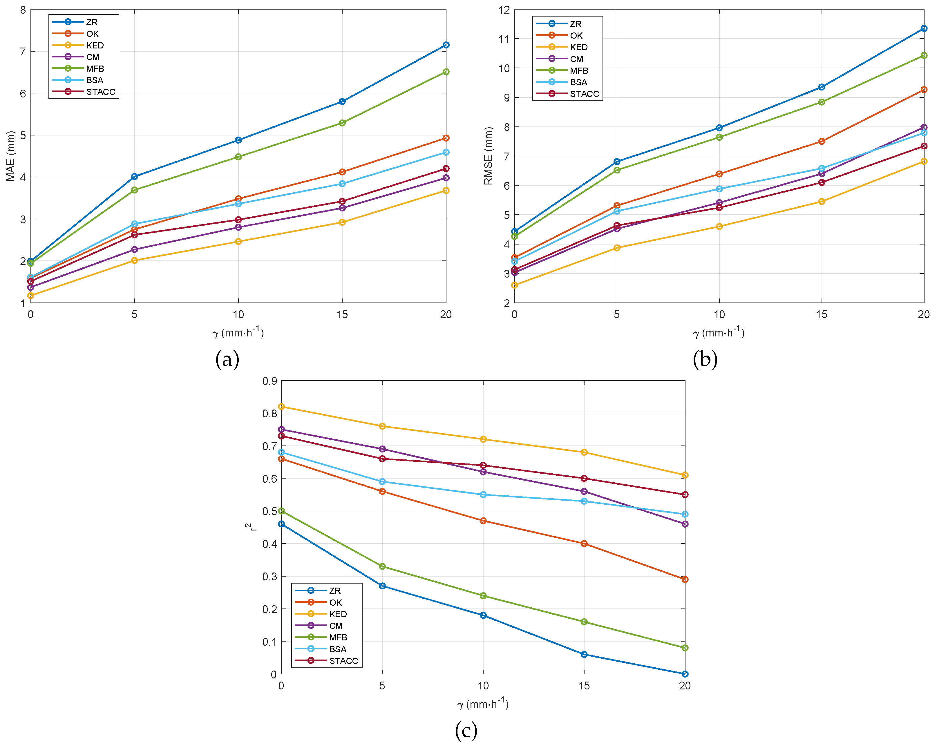
, respectively. Table 2 shows the values of the three performance metrics obtained for each method and threshold, while Figure 6 shows, for each method, the trends of these metrics vs.

γ

. From these results, we observe that ZR remains the least effective among all QPE methods, especially at the highest values of

γ

, for which the

r^{2}

value drops to zero. Regarding the fusion-based methods, MFB again provides the poorest performance (with

r^{2}

approaching zero), while KED continues to demonstrate the best results. As the threshold level increases, the improvement of the fusion-based methods over single-source ones becomes more pronounced, especially in terms of RMSE and

r^{2}

3.2. Analysis with Missing Data: Case 1

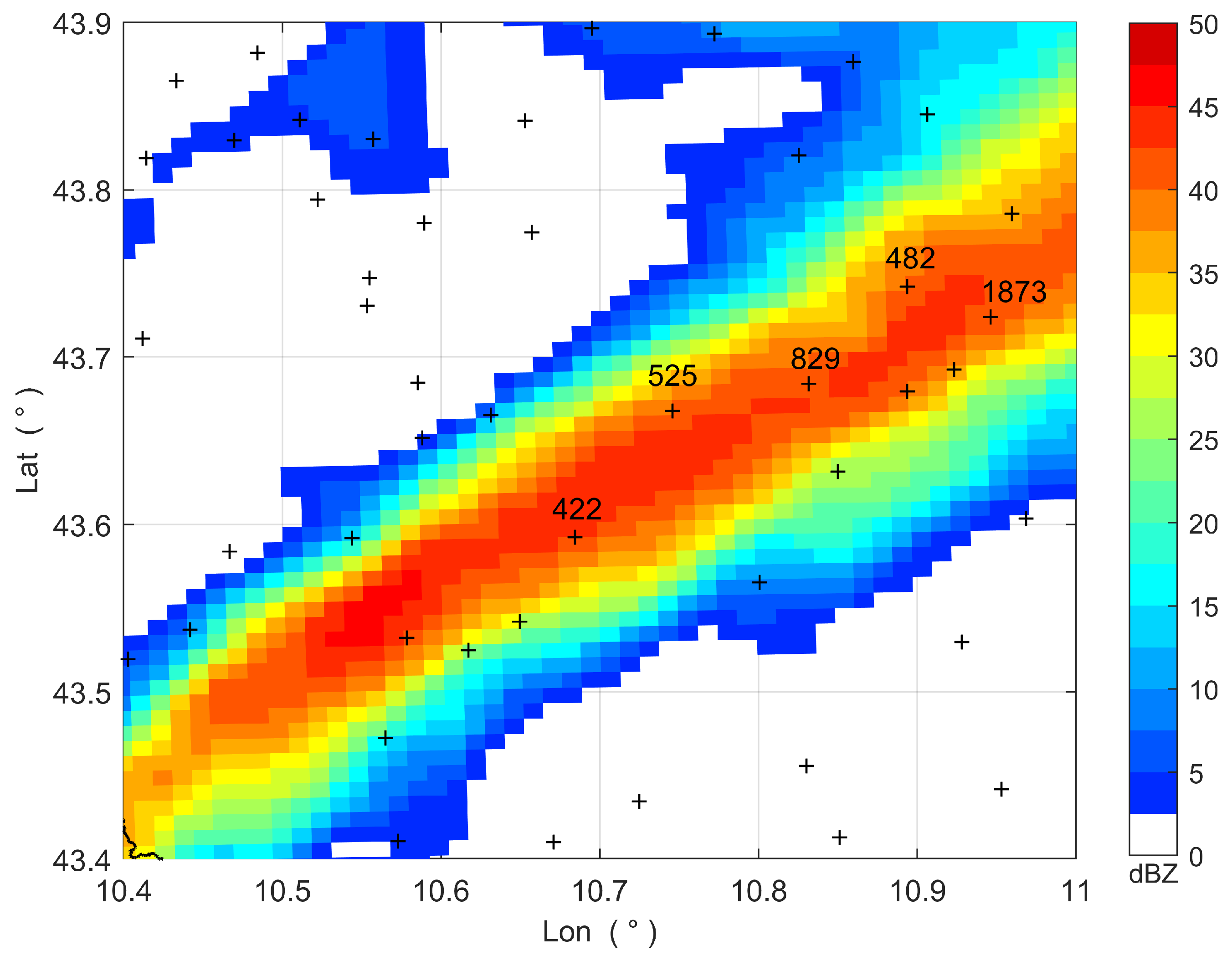
Figure 7 shows the radar reflectivity map, space-time averaged from 15:30 UTC to 16:30 UTC. The rain gauges labeled with numbers represent the ones that measured the highest rainfall levels during this time interval, with rain gauge #525 recording the greatest amount (56.80 mm); it is evident that these rain gauges are also located, as expected, in high radar reflectivity areas. 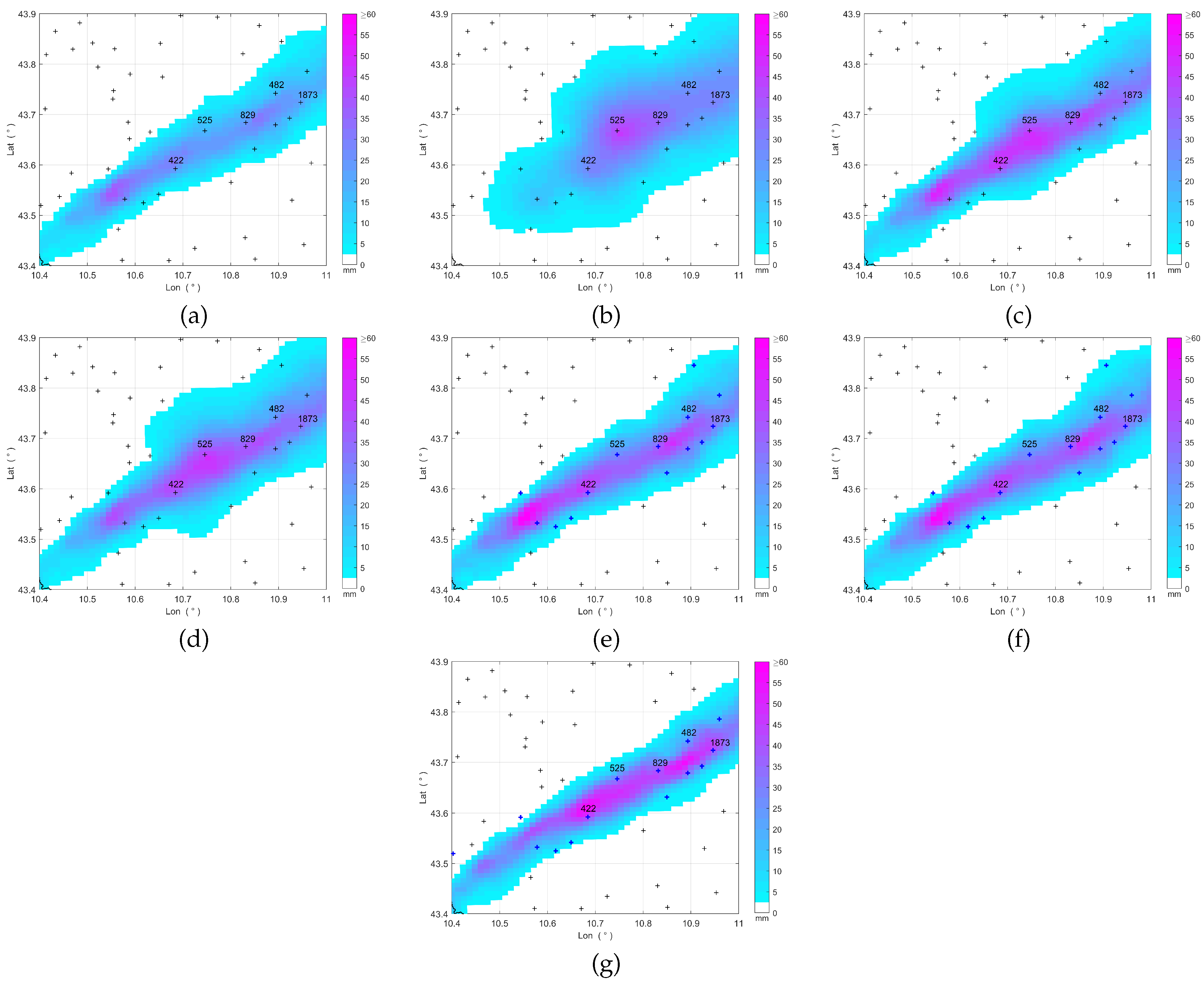The maps illustrated in Figure 8 display the rainfall accumulated over the same time interval, as estimated through the various QPE methods. In the maps obtained by MFB, BSA, and STACC the rain gauges that were actually used, i.e. those considered acceptable (see Section 2.3.5 and Section 2.3.7), are indicated by blue crosses.

To simulate and analyse a critical scenario (Section 2.4), we removed rain gauge #525 and estimated the rainfall y at its location by using the different QPE methods. We then compared these estimates to the actual measured value and computed the estimation error e to evaluate the accuracy of each method. The estimation errors are reported in Table 3. All the QPE methods underestimate the actual amount of rainfall, with the single-source estimation methods (OK and ZR) yielding, as expected, the largest errors (65.39% and 67.78%, respectively). The poor performance of these methods is inherited by methods that use geostatistical interpolation (KED and CM): in this case, the additional spatial information coming from radar is insufficient to compensate for the inaccuracy coming from rain gauges.

The ZR underestimation affects also the radar bias adjustment methods, i.e. MFB and BSA. For instance, in the BSA case, a large adjustment factor would be needed in the position of raingauge #525 to compensate for the radar underestimate. Instead, one gets the interpolation of smaller correction factors computed at the surrounding rain gauges. Similar considerations can be made for MFB.

The smallest error (27.73%) is achieved by the STACC method. Probably, the reason lies in the fusion approach of the STACC. When rain gauge #525 is removed, the Z–R relation coefficients at its location are determined by spatial interpolation of the coefficients calibrated at the surrounding rain gauge positions. Since the calibration is performed using linear regression, the resulting relationship, although based on smaller values of Z and R, can still be effectively applied to higher values of these quantities.

The simulation was repeated by removing also the other labeled rain gauges (i.e., #422, #829, #482, #1873) to further amplify the impact of missing data in the analysed high rainfall area. As shown in Table 4, removing these additional rain gauges negatively impacts all methods except for ZR, which depends only on radar data, and STACC. As expected, OK is significantly impacted, resulting in an error of 90.00 %, which consequently affects KED and CM results. MFB and BSA provide a slightly worse estimates, since, due to the aforementioned reasons, the adjustment factor is further underestimated. On the contrary, despite the removal of additional rain gauges, the STACC estimate error slightly decreases, confirming the low sensitivity of this fusion approach to the absence of rain gauges in areas featuring high levels of precipitation.

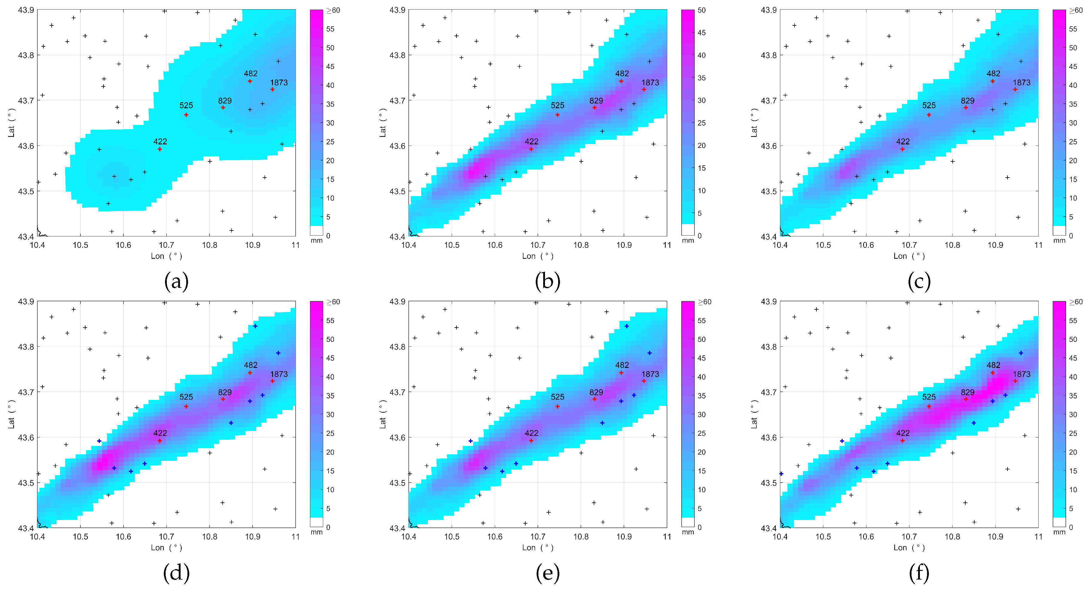
For the sake of completeness, the accumulated rainfall maps obtained by removing the labeled rain gauges are shown in Figure 9 (the map obtained by means of the ZR method is not included because it does not differ from the one shown in Figure 8). By comparing Figure 8 with Figure 9, it can be observed how the removal of the rain gauges affects the rainfall estimation results, both in terms of quantitative precision and spatial pattern.

3.3. Analysis with Missing Data: Case 2

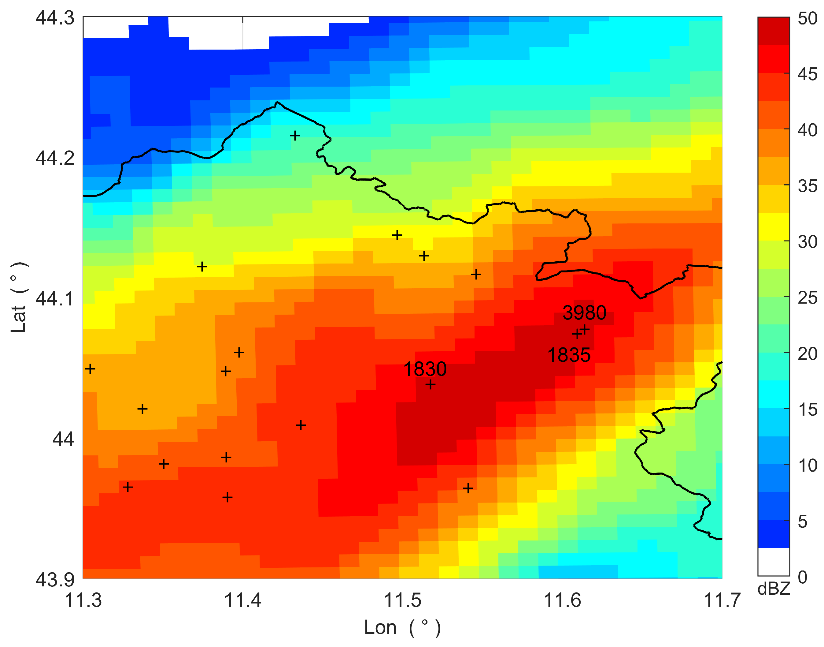
Figure 10 shows the space-time averaged radar reflectivity from 16:30 UTC to 17:30 UTC. The rain gauges labeled with numbers represent those that measured the highest rainfall levels during this time interval, with rain gauges #3980 and #1835 – which are very close to each other – recording the greatest amount (both 44.00 mm). These rain gauges are situated in an area with very high reflectivity, the highest on the map (about 50 dBZ). 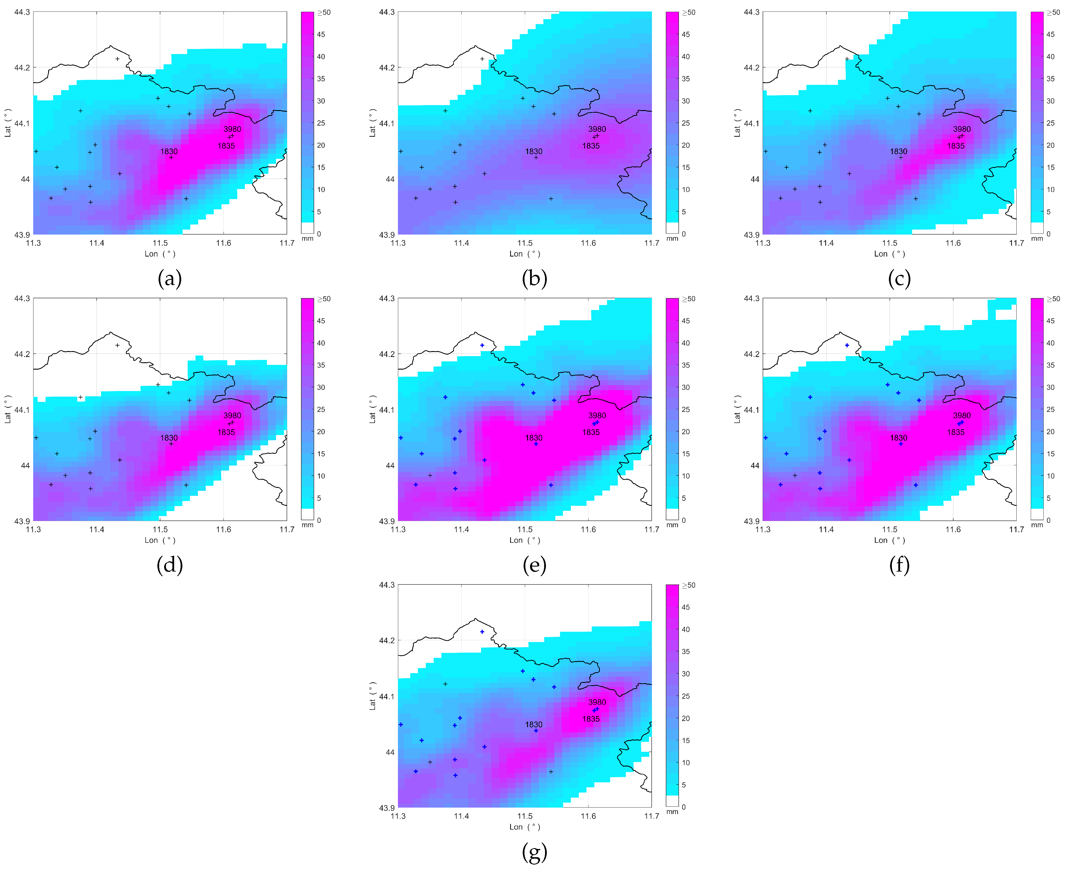The maps illustrated in Figure 11 display the rainfall accumulated over the time interval, as estimated by the various QPE methods. As in Figure 8 and Figure 9, the blue crosses in the maps related to MFB, BSA, and STACC indicate the acceptable rain gauges that were actually used.

In a similar way as what presented in Section 3.2, we simulated a critical scenario by removing rain gauges #3980 and #1835. The performance of each QPE method was then assessed by calculating the rainfall amount y at their locations and the error e between these estimates and the actual values. Table 5 presents the estimation errors obtained from these simulations. In this case, OK again tends to underestimate the actual level of rainfall for both rain gauges, but, unlike the previous simulation, the ZR method leads to an overestimate due to the very high radar reflectivity associated with the rain gauge locations and the chosen Z–R relationship; this influences on the results relative to KED, CM, MFB, and BSA. In KED and CM, the additional spatial information provided by the radar helps to correct the underestimation from the rain gauges, leading to very good results for KED, and results for CM similar to ZR. Concerning MFB and STACC, the overestimation of the ZR method is further amplified by the application of the adjustment factor, resulting in high errors (more than 100% for MFB). As in the previous simulation, the STACC method yields the best results, with errors of 5.52% and 1.91% for rain gauges #1835 and #3980, respectively, demonstrating again to be the most robust among all the analysed methods.

We also repeated the simulation by removing rain gauge #1830 as well, thereby increasing the effect of missing measurements. The results in Table 6 show that all the methods, except for ZR, lead to large errors, intensifying either the underestimation (for OK) or the overestimation (for all the other methods). In particular, KED seems to be the most affected method by the removal of rain gauge #1830, showing the largest increase in terms of relative error (e.g., from 11.55% to 97.80% for rain gauge #1835). Despite a loss of performance, the STACC method still provides good results and confirms to be the most robust method in this simulation.

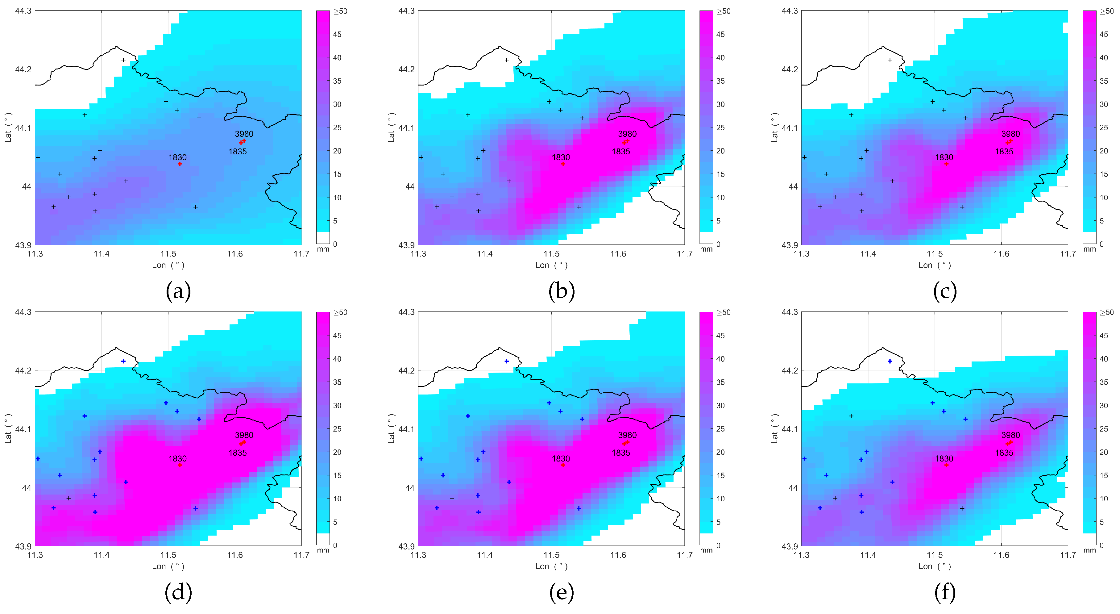
As we did for the previous simulation, we derived the accumulated rainfall maps after removing the specified rain gauges. The results are shown in Figure 12.

4. Conclusions

In this paper, a comprehensive comparison of different QPE methods based on rain gauge and weather radar data has been presented. To this aim, data collected during a severe rainfall event occurred in Tuscany, Italy were employed.

We performed a LOOCV to assess the accuracy and the reliability of each considered method. The results have shown that relying exclusively on radar data leads to quantitatively inaccurate predictions, as expected. Additionally, using the MFB method – which integrates rain gauge data by simply applying a constant adjustment factor to the radar-based rainfall field – does not significantly enhance the estimation accuracy. The results have also demonstrated that a sufficiently dense rain gauge network, such as the one in Tuscany, can produce good results even when it is utilized alone, without the radar data, as is done in the OK method. In general, however, fusion methods, like KED, CM, BSA, and STACC, allows better results than OK (with reference to the used performance metrics MAE, RMSE, and

r^{2}

) to be achieved, especially when considering rain gauges that recorded a certain level of rainfall. Among these methods, KED, which belongs to the geostatistical interpolation fusion method category and thus benefits from the dense rain gauge network, has proven to be the most effective QPE method in this context, providing the best performance in terms of all the metrics.

A second type of analysis was also carried out, trying to highlight the robustness of the QPE methods in critical situations, in which high rainfall areas might occur in regions low-populated in terms of rain gauges. This analysis was performed by removing some rain gauges from the data available to the QPE algorithms and evaluating the estimation. This analysis disclosed, as expected, the main drawback of methods relying solely on rain gauge data and pointed out the essential role of spatial information provided by radar. Among the fusion methods, STACC demonstrated the highest robustness under these challenging conditions, yielding the smallest estimation errors.

In general, the study has highlighted the advantages of merging rain gauge data with weather radar observations to improve QPE. In fact, through the integration of these two data sources, we have achieved more accurate rainfall estimates compared to using either data source independently. The findings have offered further evidence of the validity of fusion techniques for both operational meteorology and hydrological applications, such as flood forecasting, where precise precipitation measurements are essential.

Author Contributions

Conceptualization, A.B., L.F., F.A. and F.C.; methodology, A.B., L.F., F.A. and F.C.; software, A.B. and F.C.; validation, A.B.; formal analysis, A.B., L.F. and F.A.; investigation, A.B.; resources, L.F. and F.C.; data curation, A.B.; writing—original draft preparation, A.B.; writing—review and editing, A.B., L.F. and F.A.; visualization, A.B., L.F. and F.A.; supervision, L.F. and F.A.; project administration, L.F. All authors have read and agreed to the published version of the manuscript.

Funding

This research received no external funding.

Institutional Review Board Statement

Not applicable.

Informed Consent Statement

Not applicable.

Data Availability Statement

The original contributions presented in the study are included in the article, further inquiries can be directed to the corresponding author/s.

Acknowledgments

The authors would like to thank the Italian National Civil Protection Department (DPCN) for providing the weather radar data and the LaMMA Consortium for providing rain gauge data

Conflicts of Interest

The authors declare no conflicts of interest.

References

Lanza, L.G.; Vuerich, E. The WMO Field Intercomparison of Rain Intensity Gauges. Atmospheric Research 2009, 94, 534–543. [Google Scholar] [CrossRef]
Michaelides, S.; Levizzani, V.; Anagnostou, E.; Bauer, P.; Kasparis, T.; Lane, J. Precipitation: Measurement, Remote Sensing, Climatology and Modeling. Atmospheric Research 2009, 94, 512–533. [Google Scholar] [CrossRef]
Ahrens, B. Distance in spatial interpolation of daily rain gauge data. Hydrology and Earth System Sciences 2006, 10, 197–208. [Google Scholar] [CrossRef]
Wackernagel, H. Multivariate Geostatistics: An Introduction with Applications, 3rd ed.; Springer: Heidelberg, Germany, 2003. [Google Scholar]
Piazza, A.D.; Conti, F.L.; Noto, L.V.; Viola, F.; Loggia, G.L. Comparative analysis of different techniques for spatial interpolation of rainfall data to create a serially complete monthly time series of precipitation for Sicily, Italy. International Journal of Applied Earth Observation and Geoinformation 2011, 13, 396–408. [Google Scholar] [CrossRef]
Mair, A.; Fares, A. Comparison of Rainfall Interpolation Methods in a Mountainous Region of a Tropical Island. Journal of Hydrologic Engineering 2011, 16, 371–383. [Google Scholar] [CrossRef]
Doviak, R.J.; Zrnić, D.S. Doppler Radar and Weather Observations, 2nd ed.; Academic Press: San Diego, CA, USA, 1993. [Google Scholar]
Villarini, G.; Krajewsky, W.F. Review of the Different Sources of Uncertainty in Single Polarization Radar-Based Estimates of Rainfall. Surveys in Geophysics 2010, 31, 107–129. [Google Scholar] [CrossRef]
Wilson, J.W.; Brandes, E.A. Radar Measurement of Rainfall—A Summary. Bulletin of the American Meteorological Society 1979, 60, 1048–1060. [Google Scholar] [CrossRef]
Chapon, B.; Delrieu, G.; Gosset, M.; Boudevillain, B. Variability of rain drop size distribution and its effect on the Z–R relationship: A case study for intense Mediterranean rainfall. Atmospheric Research 2008, 87, 52–65. [Google Scholar] [CrossRef]
Smith, J.A.; Hui, E.; Steiner, M.; Baeck, M.L.; Krajewski, W.F.; Ntelekos, A.A. Variability of rainfall rate and raindrop size distributions in heavy rain. Water Resources Research 2009, 45. [Google Scholar] [CrossRef]
Atlas, D.; Ulbrich, C.W.; Meneghini, R. The multiparameter remote measurement of rainfall. Radio Science 1984, 19, 3–22. [Google Scholar] [CrossRef]
Lee, G.W.; Zawadzki, I. Variability of Drop Size Distributions: Time-Scale Dependence of the Variability and Its Effects on Rain Estimation. Journal of Applied Meteorology 2005, 44, 241–255. [Google Scholar] [CrossRef]
Ochoa-Rodriguez, S.; Wang, L.P.; Willems, P.; Onof, C. A Review of Radar-Rain Gauge Data Merging Methods and Their Potential for Urban Hydrological Applications. Water Resources Research 2019, 55, 6356–6391. [Google Scholar] [CrossRef]
Sinclair, S.; Pegram, G. Combining radar and rain gauge rainfall estimates using conditional merging. Atmospheric Science Letters 2005, 6, 19–22. [Google Scholar] [CrossRef]
Brandes, E.A. Optimizing Rainfall Estimates with the Aid of Radar. Journal of Applied Meteorology and Climatology 1975, 14, 1339–1345. [Google Scholar] [CrossRef]
Cuccoli, F.; Facheris, L.; Antonini, A.; Melani, S.; Baldini, L. Weather Radar and Rain-Gauge Data Fusion for Quantitative Precipitation Estimation: Two Case Studies. IEEE Transactions on Geoscience and Remote Sensing 2020, 58, 6639–6649. [Google Scholar] [CrossRef]
Biondi, A.; Facheris, L.; Argenti, F.; Cuccoli, F.; Antonini, A.; Melani, S. Assessing quantitative precipitation estimation methods based on the fusion of weather radar and rain-gauge data. IEEE Geoscience and Remote Sensing Letters 2024, 21, 1–5. [Google Scholar] [CrossRef]
Report Meteorologico: Evento 2 novembre 2023 (Consorzio LaMMA). Available online (in Italian): https://www.lamma.toscana.it/clima/report/eventi/evento_02112023.pdf (accessed on August 2, 2024).
Vulpiani, G.; Montopoli, M.; Passeri, L.D.; Gioia, A.G.; Giordano, P.; Marzano, F.S. On the Use of Dual-Polarized C-Band Radar for Operational Rainfall Retrieval in Mountainous Areas. Journal of Applied Meteorology and Climatology 2012, 51, 405–425. [Google Scholar] [CrossRef]
Meteo-Hub Mistral (Meteo Italian Supercomputing Portal). Available online: https://meteohub.mistralportal.it/app/datasets (accessed on July 26, 2024).
Zhang, J.; Howard, K.; Langston, C.; Kaney, B.; Qi, Y.; Tang, L.; Grams, H.; Wang, Y.; Cocks, S.; Martinaitis, S.; Arthur, A.; Cooper, K.; Brogden, J.; Kitzmiller, D. Multi-Radar Multi-Sensor (MRMS) Quantitative Precipitation Estimation: Initial Operating Capabilities. Bulletin of the American Meteorological Society 2016, 97, 621–638. [Google Scholar] [CrossRef]
Marshall, J.; Hitschfeld, W.; Gunn, K. Advances in Radar Weather. Advances in Geophysics 1955, 2, 1–56. [Google Scholar] [CrossRef]
Müller, S.; Schüler, L.; Zech, A.; Heße, F. GSTools v1.3: a toolbox for geostatistical modelling in Python. Geoscientific Model Development 2022, 15, 3161–3182. [Google Scholar] [CrossRef]
Goudenhoofdt, E.; Delobbe, L. Evaluation of radar-gauge merging methods for quantitative precipitation estimates. Hydrology and Earth System Sciences 2009, 13, 195–203. [Google Scholar] [CrossRef]
Orear, J. Least squares when both variables have uncertainties. American Journal of Physics 1982, 50, 912–916. [Google Scholar] [CrossRef]
Battan, L.J. Radar observation of the atmosphere. Quarterly Journal of the Royal Meteorological Society 1973, 99, 793–793. [Google Scholar] [CrossRef]
Shepard, D. A two-dimensional interpolation function for irregularly-spaced data. 23rd ACM National Conference, 1968, p. 517–524. [CrossRef]

Figure 1. Instability fronts and lines, November 2, 2023: (a) 12:00 UTC; (b) 18:00 UTC (Source: MetOffice, U.K.). The instability line affecting Tuscany is circled in black. The figures are taken from [19].

Figure 2. Convective available potential energy (CAPE), November 2, 2023: (a) 15:00 UTC; (b) 18:00 UTC. The figures are taken from [19].

Figure 3. Radar systems of the Italian National weather radar network that cover Tuscany. The red asterisks mark the radar sites, while the black lines indicate the Italian regional boundaries (Tuscany is highlighted in orange).

Figure 4. CAPPI product at a height of 2000 m on November 2, 2023: (a) 16:00 UTC; (b) 17:00 UTC; (c) 18:00 UTC; (d) 19:00 UTC. The black lines mark the boundary of the the Tuscany region.

Figure 5. Rain gauge network of Tuscany (total number of gauges: 425). Each rain gauge location is marked by a red dot, while the black lines indicate the regional boundaries of Tuscany. The study area is represented by the cyan polygon and contains 323 rain gauges.

Figure 6. Trend of (a) MAE, (b) RMSE, and (c)

r^{2}

as a function of the threshold

γ

Figure 6. Trend of (a) MAE, (b) RMSE, and (c)

r^{2}

as a function of the threshold

γ

Figure 7. Space-time averaged radar reflectivity from 15:30 UTC to 16:30 UTC, November 2, 2023. The crosses mark the rain gauge locations.

Figure 8. Accumulated rainfall maps from 15:30 UTC to 16:30 UTC, November 2, 2023, obtained by using: (a) ZR, (b) OK, (c) KED, (d) CM, (e) MFB, (f) BSA, (g) STACC. The crosses mark the rain gauge locations.

Figure 9. Accumulated rainfall maps from 15:30 UTC to 16:30 UTC, November 2, 2023, obtained by removing data of the labeled rain gauges and by using: (a) OK, (b) KED, (c) CM, (d) MFB, (e) BSA, (f) STACC. The crosses mark the rain gauge locations (the red ones indicate the removed rain gauges).

Figure 10. Space-time averaged radar reflectivity from 16:30 UTC to 17:30 UTC, November 2, 2023. The crosses mark the rain gauge locations, while the black line represents the boundary of the Tuscany region.

Figure 11. Accumulated rainfall maps from 16:30 UTC to 17:30 UTC, November 2, 2023, obtained by using: (a) ZR, (b) OK, (c) KED, (d) CM, (e) MFB, (f) BSA, (g) STACC. The crosses mark the rain gauge locations, while the black line represents the boundary of the Tuscany region.

Figure 12. Accumulated rainfall maps from 16:30 UTC to 17:30 UTC, November 2, 2023, obtained by removing data of the labeled rain gauges and by using: (a) OK, (b) KED, (c) CM, (d) MFB, (e) BSA, (f) STACC. The crosses mark the rain gauge locations (the red ones indicate the removed rain gauges), while the black line represents the boundary of the Tuscany region.

Table 1. Leave-one-out cross-validation results:

T = 5

h (from 15:30 UTC to 20:30 UTC),

T_{s} = 30

min.

Table 1. Leave-one-out cross-validation results:

T = 5

h (from 15:30 UTC to 20:30 UTC),

T_{s} = 30

min.

Method	MAE (mm)	RMSE (mm)	$r^{2}$
ZR	1.99	4.43	0.46
OK	1.59	3.54	0.66
KED	1.17	2.60	0.82
CM	1.37	3.03	0.75
MFB	1.94	4.26	0.50
BSA	1.61	3.41	0.68
STACC	1.51	3.13	0.73

Table 2. Leave-one-out cross-validation results when a threshold

γ

is set:

T = 5

h (from 15:30 UTC to 20:30 UTC),

T_{s} = 30

min.

Table 2. Leave-one-out cross-validation results when a threshold

γ

is set:

T = 5

h (from 15:30 UTC to 20:30 UTC),

T_{s} = 30

min.

Method	MAE (mm)				RMSE (mm)				$r^{2}$
Method	$γ_{1}$	$γ_{2}$	$γ_{3}$	$γ_{4}$	$γ_{1}$	$γ_{2}$	$γ_{3}$	$γ_{4}$	$γ_{1}$	$γ_{2}$	$γ_{3}$	$γ_{4}$
ZR	4.01	4.88	5.80	7.15	6.81	7.96	9.35	11.35	0.27	0.18	0.06	0.00
OK	2.75	3.48	4.12	4.93	5.31	6.39	7.50	9.26	0.56	0.47	0.40	0.29
KED	2.01	2.46	2.92	3.68	3.87	4.60	5.45	6.82	0.76	0.72	0.68	0.61
CM	2.27	2.80	3.26	3.98	4.52	5.41	6.40	7.98	0.69	0.62	0.56	0.46
MFB	3.69	4.48	5.29	6.51	6.52	7.64	8.84	10.43	0.33	0.24	0.16	0.08
BSA	2.88	3.36	3.84	4.59	5.12	5.88	6.58	7.79	0.59	0.55	0.53	0.49
STACC	2.62	2.98	3.42	4.20	4.63	5.24	6.10	7.34	0.66	0.64	0.60	0.55

Table 3. Case 1: estimation errors obtained removing rain gauge #525.

Method	y (mm)	e (mm)	$e_{%}$
ZR	19.66	−37.14	65.39%
OK	18.30	−38.50	67.78%
KED	27.13	−29.67	52.24%
CM	25.31	−31.49	55.44%
MFB	29.62	−27.18	47.85%
BSA	28.15	−28.65	50.44%
STACC	41.05	−15.75	27.73%

Table 4. Case 1: estimation errors when also rain gauges #422, #829, #482, and #1873 are removed.

Method	y (mm)	e (mm)	$e_{%}$
ZR	19.66	−37.14	65.39%
OK	5.68	−51.12	90.00%
KED	22.20	−34.60	60.92%
CM	20.24	−36.56	64.37%
MFB	29.38	−27.43	48.29%
BSA	26.37	−30.43	53.57%
STACC	42.53	−14.27	25.12%

Table 5. Case 2: estimation errors obtained removing rain gauges #3980 and #1835.

Method	y(mm)		e(mm)		$e_{%}$
Method	#1835	#3980	#1835	#3980	#1835	#3980
ZR	65.48	55.10	21.48	11.10	48.82%	25.23%
OK	21.44	21.03	−22.56	−22.97	51.27%	52.20%
KED	49.08	41.86	5.08	−2.14	11.55%	4.86%
CM	66.01	55.72	22.01	11.72	50.02%	26.64%
MFB	113.06	95.15	69.06	51.15	156.95%	116.25%
BSA	86.93	73.04	42.93	29.04	97.57%	66.00%
STACC	46.43	43.16	2.43	−0.84	5.52%	1.91%

Table 6. Case 2: estimation errors obtained when also rain gauge #1830 is removed.

Method	y (mm)		e (mm)		$e_{%}$
Method	#1835	#3980	#1835	#3980	#1835	#3980
ZR	65.48	55.10	21.48	11.10	48.82%	25.23%
OK	17.22	17.01	−26.78	−26.99	60.86%	61.34%
KED	87.03	73.18	43.03	29.18	97.80%	66.32%
CM	68.09	57.74	24.09	13.74	54.75%	31.23%
MFB	119.62	100.66	75.62	56.66	171,86%	128.77%
BSA	91.81	77.23	47.81	33.23	108.66%	75.52%
STACC	52.67	47.24	8.67	3.24	19.70%	7.36%

Disclaimer/Publisher’s Note: The statements, opinions and data contained in all publications are solely those of the individual author(s) and contributor(s) and not of MDPI and/or the editor(s). MDPI and/or the editor(s) disclaim responsibility for any injury to people or property resulting from any ideas, methods, instructions or products referred to in the content.

© 2024 by the authors. Licensee MDPI, Basel, Switzerland. This article is an open access article distributed under the terms and conditions of the Creative Commons Attribution (CC BY) license (http://creativecommons.org/licenses/by/4.0/).

Copyright: This open access article is published under a Creative Commons CC BY 4.0 license, which permit the free download, distribution, and reuse, provided that the author and preprint are cited in any reuse.

MDPI Initiatives

Important Links

Choose an area of interest and we will send you notifications of new preprints at your preferred frequency.

Disclaimer

Comparison of Different Quantitative Precipitation Estimation Methods Based on a Severe Rainfall Event in Tuscany, Italy, November 2023

Abstract

1. Introduction

2. Materials and Methods

2.1. Meteorological Event Description

2.2. Datasets

2.2.1. Radar Dataset

2.2.2. Rain Gauge Dataset

2.3. QPE Methods

2.3.1. Radar-Based Method

2.3.2. Rain Gauge-Based Method

2.3.3. Kriging With External Drift (KED)

2.3.4. Conditional Merging (CM)

2.3.5. Mean Field Bias Adjustment (MFB)

2.3.6. Brandes Spatial Adjustment (BSA)

2.3.7. Space-Time Conversion Coefficients (STACC)

2.4. Performance Analysis

3. Experimental Results and Discussion

3.1. Leave-One-Out Cross-Validation (LOOCV)

3.2. Analysis with Missing Data: Case 1

3.3. Analysis with Missing Data: Case 2

4. Conclusions

Author Contributions

Funding

Institutional Review Board Statement

Informed Consent Statement

Data Availability Statement

Acknowledgments

Conflicts of Interest

References

MDPI Initiatives

Important Links

Subscribe