
Submitted:
17 September 2024
Posted:
18 September 2024
You are already at the latest version
Abstract
Amethod for the certification of local and almost global stability of invariant sets of ordinary differential equations on torus is proposed. The method is based on using trigonometric polynomials as candidates of local Lyapunov functions or (global) Lyapunov densities (so-called dual Lyapunov functions) and converting the required local Lyapunov or dual Lyapunov conditions into semidefinite programming. We provide several examples with three and four oscillators to showcase the adaptability of our results, which can be used to certify partial or complete phase-locking/phase-cohesion and to validate the presence of an attracting/repelling set in various scenarios.
Keywords:
almost global synchronization
; trigonometric polynomials
; stability certificates
1. Introduction
Current stability methods are still improving for dynamical systems such as humanoid robots and unmanned aerial vehicles, which are becoming increasingly prominent in today’s technology. The techniques that have been developed are available for very special classes of systems or are based on heuristic methods. With the increased computer processing power, algorithmic optimization methods have recently been developed to stabilize dynamic systems.
Lyapunov stability theorems are extensively utilized in the design of stabilizing feedback for various applications, including path-following robots [1], stabilization of fixed-wing unmanned aerial vehicles (UAV) [2], circular motion stability in UAV [3], unmanned surface vehicles [4], and magnetic field-operated satellites using the sum of squares method (SOS) [5]. Using the global Lyapunov functions, a closed-loop control system can reach a desired equilibrium point under every initial condition. However, two difficulties arise here: First, the global Lyapunov method can only directly be applied to systems on an Euclidean space [6]. For an equilibrium point to be globally stable in smooth vector fields, the state space must be equivalent (homeomorphic) to an Euclidean space [7]. In contrast, state space of a rotational dynamical system is often a multidimensional torus (for systems described by angular dynamical variables only) or a multidimensional cylinder (for systems described by both angular and non-angular variables). For such systems, it is not possible to stabilize an equilibrium point globally with continuous state feedback. The dual-Lyapunov method was introduced in [8] to overcome the two difficulties encountered while applying the global Lyapunov theorem. Whereas the Lyapunov method uses a continuous function decreasing along the singular solutions as a certificate of stability, the dual-Lyapunov method uses an increasing density function (Lyapunov density) along the solution sets as a certificate of almost global stability. Another difference between the two methods is that the dual-Lyapunov theorem guarantees convergence for almost every initial condition, while the global Lyapunov stability theorem guarantees that the solutions converge to an equilibrium point for every initial condition. [6,8] state that stability certification with the dual-Lyapunov theorem may be more advantageous than the classical Lyapunov method for systems expressed in angular variables. In [9], it was shown that the dual-Lyapunov method is more suitable for design with linear matrix inequalities since it requires an inequality that depends linearly on the design quantities, unlike the conventional Lyapunov method.
Since in rotational systems, the non-angular variables (e.g., angular velocity) depend on the angular variables (e.g., angle), fixing the angular variables at a value means convergence of the non-angular variables. More precisely, since angular state variables define a bounded manifold such as a torus, and since every continuous function (e.g., polynomials) on a bounded manifold is integrable, it may be possible to propose a systematic dual-Lyapunov design method for angular state variables in a polynomial approach. In this study, both the conventional local Lyapunov functions and the (global) Lyapunov density have been used to certify local stability and almost global stability, respectively, of an equilibrium or of a limit cycle. The polynomial approximation method based on the sum of squares (SOS) and semidefinite programming (SDP) [10], widespread in the literature in the last 20 years, the trigonometric polynomials [11], which has primary applications in signal processing, is used. SDP formulations of positive trigonometric polynomials have been utilized in signal processing applications such as FIR (finite impulse response) filters [12], beamformers [13], adapted wavelets [14], compaction filters [15] etc. In control engineering, trigonometric polynomials have been used in stability analysis of discrete-time systems [16].
In this work, we present the certifications of the almost global stability of dynamical systems on hypertorus in Theorem 1, in Section 3 by using Gram matrices and trace parametrizations of trigonometric polynomials. We use this theory to certify some physical phenomenons of coupled oscillators such as the almost global phase synchronization of uniform all-to-all coupled three oscillators in Example 1, the almost global phase-locking in three nonuniform coupled oscillators in Example 3, the almost global partial-phase-cohesion in nonuniform Kuramoto model with a tree-topology in Example 4. Using Gram matrices of trigonometric polynomials, we improve a technique for the certification of local Lyapunov stability of systems on hypertorus by using Putinar’s Positivstellensatz Lemma 2 in Theorem 2 in Section 3. We employ Theorem 2 to certify the local Phase Synchronization of uniform all-to-all coupled Oscillators for three and four oscillators in Example 2.
2. Preliminaries
2.1. Trigonometric Polynomials
A trigonometric polynomial is defined by
where is the degree of the trigonometric polynomial, ; ; and are complex coefficients of . Observe the difference in how the elements of are denoted depending on whether they represent degrees or indices. We make this distinction to make tracking of indices throughout the paper easier. Here, is an inner product. For real-valued a trigonometric polynomial , the coefficients must satisfy the symmetry (Hermitian) condition where denotes the complex conjugate of x,11]. The inequality is understood elementwise and is equivalently denoted by and . We denote the vectors by 0 and 1 respectively; and .
The Gram matrix associated with is defined by
where is a square matrix of size , is a vector composed of monomials from the trigonometric basis on , and is its conjugate transpose. In particular, .
If the Gram matrix is positive semidefinite, then ,17]. Even more can be said in this case. Any positive semidefinite matrix can be decomposed as for some upper triangular matrix U, known as its Cholesky decomposition. This implies that for some upper triangular matrix U, hence can be expressed as a sum of squares (SOS) which are defined to have a general form
where each is a trigonometric polynomial.
Toeplitz matrices occur frequently in the study of trigonometric polynomials. An matrix T is said to be the elementary Toeplitz matrix of size n if it is a matrix with ones on the diagonal, meaning if and only if . We will denote the elementary Toeplitz matrix of size n by . Clearly, is a zero matrix for any . Define where ⊗ denotes the Kronecker product. If , then for some i. In that case , hence , is the zero matrix. Toeplitz matrices are utilized to relate the coefficients of to the Gram matrix in (2) by a property known in the literature as trace parameterization [11], which states for any
Positive semidefinite matrices can parametrize SOS trigonometric polynomials [11,18]. Equivalently, is SOS if and only if there exits positive semidefinite Gram matrix in (2) satisfying (4) (Theorem 3.15, [11]).
Given the trigonometric polynomial defined in (1), we can define the derivative with respect to as follows
where . Thus, due to (4) the relationship between Gram matrix of and Gram matrix of is given
where are the Toeplitz matrices corresponding to in (2).
Consider another trigonometric polynomial defined as
where are the coefficients of . The product of the polynomials and , denoted as , is also a trigonometric polynomial which can expanded as
where , and the coefficients are given by
The Gram matrix associated with the product can be expressed in terms of Gram matrices and of and , respectively. Specifically, we have
We end this section by defining a zero-sum matrix or a matrix having zero-sum. As the name suggests, all elements of such a matrix sum up to 0. If the Gram-matrix in (2) has zero-sum, then it is clear that .
2.2. A Class of Coupled Oscillators
In this article, we consider a class of coupled oscillators defined on the hypertorus as
where each component function has a Fourier series expansion
with Fourier coefficients . Without loss of generality, we can assume that all component functions can be expressed using the same number of harmonics. This can be done by taking and adding zero fourier coefficients wherever necessary. Every smooth vector field on a compact manifold is complete [19], meaning that the flow is defined for each . Thus, the solutions of (11) exist for all time, irrespective of the initial condition. A set is said to be forward-invariant (backward-invariant, respectively) under the flow of (11) if for all (, respectively). A is forward-invariant if and only if is backward-invariant.
Global (asymptotic) stability has been a well-explored issue in systems theory for the past several decades and is characterized by all solution curves converging to the equilibrium point. Due to topological restrictions, systems on a hypertorus cannot be globally asymptotically stable. However, in some cases, the system (11) might exhibit
- almost global stability: if the set of divergent solution curves (with respect to an equilibrium point) has zero measure; and
- local stability: if there exists a region such that all solution curves originating from converge to an equilibrium point in .
Another interesting notion for coupled oscillators is that of synchronization. We say that the oscillators i and j are phase synchronized if ; phase-locked if for some ; and frequency synchronized if . The system (11) is said to exhibit
- almost global phase synchronization (phase-locking, frequency synchronization, respectively): if the set of initial conditions on for which a pair of oscillators is not phase synchronized (not phase-locked, not frequency synchronized, respectively) has zero measure; and
- local phase synchronization (phase-locking, frequency synchronization, respectively): if there exists a region such that the set of initial conditions on for which a pair of oscillators is not phase synchronized (not phase-locked, not frequency synchronized, respectively) is a subset of .
Under suitable conditions, for example, in the presence of phase-shift symmetry , the system (11) on can be reduced to a phase-difference system on , refer [20]. In that case, the system (11) exhibits almost global phase synchronization (phase-locking, respectively) if and only if its corresponding phase-difference system exhibits almost global stability to the origin (to an equilibrium point , respectively). This relationship has also been briefly touched upon in Example 2 for the local counterpart of the statement.
In this article, we are interested in obtaining a certificate for almost global stability and a certificate for local stability of the sysem (11). Lyapunov method, which relies on finding an energy-like function that decreases along solution trajectories of the system, has been a tool to establish the global stability of systems. We will employ the Lyapunov method locally to establish the local stability of (11). The Lyapunov method has a sibling, the dual-Lyapunov method proposed by Rantzer (Theorem 1, [8]), which is a well-known tool to certify the almost global stability of such systems. Unlike the Lyapunov method, the dual-Lyapunov method relies on finding a `Lyapunov density’ satisfying certain density propagation inequalities. The following lemma can be seen as a modified version of Rantzer’s theorem for the system (11).
(Theorem 4.2, [21])).Lemma 1 (Adapted from Let be a compact set such that is backward-invariant under the flow of (11). If there exists a continuously differentiable function and satisfies
- C1.
- for almost every .
- C2.
- ρ is integrable away from A, that is, if
- C3.
- for almost every .
Then almost all solutions of (11) converge to A as .
Note that the flow of (11) is defined for all time; hence, the convergence of solution curves can be discussed. The second condition is a constraint on the evolution of density , whose details can be found in [8]. It is known that a density satisfying the evolution constraint inevitably has a singularity in A (Lemma 3, [21]). Considering this and taking where is a trigonometric polynomial, we obtain the following corollary.
Corollary 1.
Assume there exist nonzero trigonometric polynomials and such that is forward-invariant under the flow of (11); and for almost every
Proof.
Consider where is a nonzero trigonometric polynomial and take . A is the set of all singularities of , is a closed subset of a compact space (hence compact), and has zero measure. Thus, A is a forward-invariant compact subset under the flow of (11). This implies is a backward-invariant subset under the flow of (11). On substitution, condition C3 reduces to (13) for some nonzero trigonometric polynomial . The set of singularities of is nonempty due to Remark 3 [21], thus A is nonempty. Also, is positive on and bounded, hence integrable, over for any . Thus, conditions C1 and C2 is satisfied. Hence, by Lemma 1, almost all solutions of (11) converge to the set . □
2.2.1. Generalized Kuramoto Models with Coupling Topology
Consider the diffusively coupled system of d phase oscillators given by
where is the natural frequency of the oscillator ; is a matrix defining the coupling topology, meaning if and only if there is an edge from the oscillator to (in physical terms, influences ); K is the coupling constant; and g is a coupling function expressed in terms of its first L harmonics
where for all k. The system is called all-to-all coupled if for all . System of coupled oscillators where all oscillators have identical natural frequencies for all are called uniform coupled oscillators. It is easy to observe that all oscillators should necessarily share a common natural frequency for phase synchronization for an all-to-all connected system. Note that (14) has phase shift symmetry ; hence we reiterate that local (or almost global) synchronization can be established by proving local (or almost global) stability of its corresponding phase-difference system, refer [20] and Example 2. When , all-to-all coupled oscillators take the form of the well-known Kuramoto model
hence we refer to phase oscillator (14) as a generalized Kuramoto model with coupling topology.
When oscillators are nonuniform, that is for some pair in (14), phase synchronization is not possible. It is known that nonuniform oscillators (14) exhibit frequency synchronization for sufficiently large coupling K. Frequency synchronization is necessary for phase-locking but not sufficient. However, for the Kuramoto model (16), both are equivalent Remark 2.1 [22].
Having discussed all the prerequisites required for the paper, we present the main results in the next section.
3. Trigonometric Polynomials in Stability Analysis
In this section, we will obtain a certificate for almost global stability and a certificate for local stability of the sysem (11). The main idea is to find a Lyapunov density of the form in the former case, and a local Lyapunov function in the latter case, for some nonnegative trigonometric polynomial V. We will observe that the existence of a Lyapunov density (function, respectively) is established if the coefficients of V are zeros of some multivariate polynomial. The main problem in such a constraint is that obtaining zeroes of multivariate polynomials is extremely hard. However, trace parameterization turns the expression into a Semi-Definite Programming (SDP) problem involving matrices, the feasibility of which can be checked using solvers such as Sedumi in MATLAB. We now present our first result.
Theorem 1.
Given a dynamical system where each component function has Fourier series expansion (12), if for a nonzero Hermitian matrix of size having zero-sum, there exist a nonzero Hermitian matrix of size such that
for all , then the dynamical system satisfies Equation (13) for and corresponding to and as per (2), respectively. Subsequently, almost all solutions of (11) converge to the origin as .
Proof.
The system is almost globally stable if there exist positive definite trigonometric polynomials V and W such that and (13) is satisfied. The condition is equivalent to the sum of all entries of the Gram matrix being 0. Expanding the expression of gradient of V and divergence of F appearing in (13), we obtain that
must be satisfied. If , and denote the Gram matrices of , and respectively, the equation can be rewritten in terms of Gram matrices as
Thus, almost global stability is established if there exist positive definite matrices and satisfying the above equality and . Clearly, the size of the matrix determines the size of . Assuming that the size of is and the size of each is , the sizes of both and is . Thus, must be of the size . Thus for , by virtue of trace parametrization (4), the coefficient of both sides of (18) are equal if
□
Remark 1.
If the condition `the sum of all entries of is zero’ is dropped in Theorem 1, then . However due to [21], the trigonometric polynomial has a zero. Thus, is a nonempty compact set. If , then the set is clearly invariant under the flow of (11) and almost all solutions of (11) converge to as due to Corollary 1. In particular when is a singleton, say where is an equilibrium point of the system (11), then almost all solutions of (11) converge to as .
Given a system, the existence of a Lyapunov function, which decreases along the system’s solution trajectories, is a certificate of global stability of the system. Thus, the system (11) would be globally stable if there exists a continuously differentiable positive semidefinite function such that is negative semidefinite. Thus, to find a nonnegative trigonometric polynomial that serves as a Lyapunov function for (11), we need to find a corresponding nonnegative trigonometric polynomial satisfying
The Equation (24) also has a corresponding gram matrix representation. The equation is obtained from (13) by removing the second summand. Reproducing the steps of the proof of Theorem 1, we obtain (17) without the second summand of each term inside the bracket. We thus obtain that the expression (24) is satisfied by and if their corresponding Gram matrices and satisfy
for all . As stated before, the expression is irrelevant in establishing global stability as no system on a hypertorus is globally stable due to topological restrictions. This will, however, be used later to establish the local stability of systems on a hypertorus by considering the equality only on certain subsets of .
We now recall a celebrated result, which characterizes the trigonometric polynomials that are positive in certain domains. The domain comprises points in the state space where a given set of trigonometric polynomials is positive.
Lemma 2
(Putinar’s Positivstellensatz; adapted from [11] as per notations of this paper). Let be trigonometric polynomials (say, of degree ) with complex coefficients for and be the domain
If a trigonometric polynomial is positive on (that is, for all ), then there exist sum-of-squares polynomials for such that
Without loss of generality, it may be assumed that all trigonometric polynomials share the same degree . Also, [11] states that `the degrees of sum-of-squares polynomials may be arbitrarily high, at least theoretically.’ The lemma can be transformed in terms of Gram matrices by using trace parametrization (4) as follows:
Lemma 3
Remark 2.
A vector is said to have diameter a, which is denoted by , if . The set which is a 2d-gonal hypercylinder with “diagonal" joining and as its axis. Refer to Figure 1 (left) where , , and the region is a hexagonal cylinder. The terminology is used because all components of any given fall on an arc of length a in . In the literature [23,24], the authors study nonuniform all-to-all connected Kuramoto oscillators (16) and find conditions for frequency synchronization and local phase synchronization, respectively. They show that is forward-invariant. They subsequently find a Lyapunov function in this domain. The conditions ensure that all solutions starting in get phase synchronized.
Theorem 2.
Given a dynamical system satisfying ,where each component function has Fourier series expansion (12); be trigonometric polynomials with Gram-matrices for ; and
Proof.
We are interested in finding trigonometric polynomials and which are positive on and satisfy (24) for all . Note that each is a trigonometric polynomial of degree . Thus, by Putinar’s Positivstellensatz V and W must have the forms
and their corresponding Gram matrix representations can be obtained using Lemma 3 as
Clearly, and . Note that are zero-sum matrices, hence , for all . Thus, . Also (32) occurs as the left side of (25). For the right side, substitute the first equality in Equation (25) to obtain
Also note that must be equal to for the equality (25) to be satisfied. Now, since the equality (29) implies that is a Lyapunov function in . Along with the fact that is a forward-invariant set, we have the result.
The existence of such a forward-invariant set can be argued as follows. Once the Lyapunov function is obtained, we find a value such that . Then, the system is locally stable to the origin for all initial conditions from the set since the boundary points form a level set and the flow is inwards, by definition. □
Corollary 2.
Let be the all-to-all connected and uniform generalized Kuramoto model with the coupling function (15) with for all k. Suppose are fourier coefficients of , ; ; and . Let
If there exist zero-sum Hermitian matrices of sizes ; Hermitian matrices of sizes ; satisfing
for all , then all solutions of the system (14) originating from converge to the origin.
Proof.
We are interested in the case when (24) is satisfied for all for some . Let , then
Note that , and hence is a trigonometric polynomial of degree . Its Gram matrix is a square matrix of size and, due to trace parameterization, satisfies (4)
Thus, the expression is nonzero only on the set given in the hypothesis. We substitute the expression in (29) and observe that the index in changes to . Also, the summands of on both sides of (29) are nonzero (and equal to ) only when due to (37). Hence, the result will follow once we find a forward invariant set in .
Consider the set . Due to the analyticity of for each , following the proof of Lemma 2.1 [24], there is a dichotomy: the set either contains a limit point, in which case it is equal to and natural frequencies ; or the set is countable. We claim that the set is forward-invariant under the flow. Let , then ’s can be plotted on a nonunique arc of length which is less than . Let be the indices of occurring first and last, respectively, when we travel clockwise on the arc. Note that the choices are irrespective of the choice of arc. We extend this definition to corresponding to . We impose the positivity convention, . This means that .
Suppose are distinct, then there exists an interval on which ’s do not intersect and hence, due to the dichotomy, each is countable. This implies that functions and on the interval.
If , then for each
thus, all the cos terms appearing in the expression are nonnegative. Furthermore, and all the sin terms appearing in the expression are nonegative. Thus, is nonincreasing in . The set
hence is countable and can be rewritten as . Then and are constant in each of the intervals for (where ). We can repeat the process above to show that is continuous and piecewise decreasing on each of these intervals. Thus if any vector having distinct entries is contained in , then so is its solution trajectory.
When is such that no two oscillators are equal for all time, the same arguments as above apply since each is countable. If some oscillators coincide, there might be several choices for and at given time instants. We can choose the smallest index from for uniqueness and repeat the process by taking
Thus, is forward invariant and so is for any . We thus have forward invariance and the existence of a local Lyapunov function on the set , hence the result follows. □
Remark 3.
Choosing a larger r in Corollary 2, even though it shrinks the region where the Lyapunov function is being searched for, increases the problem’s computational complexity. Finding a local Lyapunov function for instead of r increases the number of summands on the right-hand side of (35) by
Corollary 3.
Given a dynamical system satisfying ,where each component function has Fourier series expansion (12); and . Let
If there exist zero-sum Hermitian matrices of sizes ; Hermitian matrices of sizes satisfying
Proof.
The region defined by is a d-dimensional ellipsoid centered at the origin, which contracts as we increase ; refer to Figure 1 (right). By definition of , we can observe that . Let be its Gram-matrix, then we have
Hence, the result follows from Theorem 2 by rewriting the expression (29). □
Remark 4.
Since the domain in Corollary 3 is constrained by the positivity of exactly one trigonometric polynomial, the computational power required to check the feasibility is sufficiently less. Also, checking for feasibility in a larger or smaller local region does not affect the computation time significantly since the same number of computations are required irrespective of the value of ε unlike for the case discussed in Remark 3.
4. Examples
We now present several examples of coupled systems with three and four oscillators, showcasing the usefulness of our results. Apart from almost global and local results for stability, synchrony, and phase-locking, the results can also be employed to validate the presence of an attracting/ repelling set, phase cohesion, and partial phase-locking of almost all solutions.
Example 1
(Almost global phase Synchronization of uniform all-to-all coupled Oscillators). Consider a system of all-to-all uniformly coupled oscillators. This system under the transformation , reduces to
We now exhibit the employment of Theorem 1 to establish the almost global phase synchronization of (38). For this, we consider a well-known coupling function g occurring in [25,26] defined by
where and . Suppose there are three oscillators (). Taking phase-difference variables , , we obtain the reduced phase-difference system of Kuramoto oscillators generated by (39) as
where . Almost global phase synchronization of (38) is equivalent to almost global stability of the phase-difference system. The Fourier (exponential) coefficients of the component functions (40) and (41) can be written in the form of matrices such that and for as follows
For and , employing Theorem 1 with SOS approach we obtain positive semidefinite Hermitian matrices and . Using the standard basis of trigonometric polynomials defined as , we obtain our Mathematica code [LINK HERE]. The expression is omitted here due to its large size; nonetheless, one such expression will be presented later.
Employing Theorem 1 with SOS approach using our GitHub code, we can obtain positive semidefinite matrices and satisfying (17) for several parameters of (44). Due to Theorem 1, almost all solutions of the phase-difference system (44) converge the origin for these parameters . These parameters values indicated in Figure 2 with blue stars give rise to complete phase synchronization of the coupled oscillators (40) and (41). The region examined in [25] is bounded by the red curve , where , .
Figure 2 demonstrates that our approach in Theorem 1 efficiently ensures almost global phase synchronization of the system (44) for parameters by producing Lyapnunov densities. Using our method, we can produce Lyapunov densities in the whole region where the almost global phase synchronization of the system (44) has already been established in [25].
The above method can also obtain Lyapunov density for identical oscillators where the connection topology is arbitrary, such as when the underlying topology is a spanning tree. It is known that such a topology gives rise to almost global phase synchronization when all subsystems have identical natural frequencies [27]. Note that the above results were proved without using the dual-Lyapunov method.
Example 2
(Local Phase Synchronization of uniform all-to-all coupled Oscillators for and ).
Consider the system (38) of three oscillators with coupling function . To certify the local synchronization of the system (38), we employ Theorem 2. Note that the coefficient of in (39) is negative, so the forward-invariance of arcs is not easy to prove mathematically, hence Corollary 2 cannot be used directly. We aim to use the equalities implying the existence of a local Lyapunov function for the phase-difference system (40) and (41) in the domain
Of course, the equalities reduce to ones obtained in Corollary 2 for this domain. The region is plotted in Figure 3 (left). We refer to this figure for the following argument. Using the equalities, we use our code to obtain a local Lyapunov function for the phase-difference system (40) and (41), but it has been skipped due to space constraints. The set is not invariant under the phase-difference flow, as seen in the figure. The subset (of the space of phase-differences) given by
is forward-invariant but is not easy to prove mathematically. Computations show that . By the definition of the Lyapunov function, we know that all vectors on the boundary satisfy and point inwards to the region. Hence, is a forward-invariant set. Thus, local stability of the phase-difference system follows.
We claim that the local stability of phase-difference system in implies that the original system exhibits local phase synchronization for initial conditions from the set
The system of phase-differences defined by (40) and (41) is obtained on realizing the phase-shift symmetry in the system (38). The phase-shift symmetry means that the vector field is invariant under the translation and does not change in the direction of the main diagonal (vector joining to ). Define an equivalence relation ∼ in as if and only if for some . Thus, the phase-difference vector field on the quotient space is obtained by projecting the original vector field to any plane perpendicular to the main diagonal. The invariance of under the phase-difference system is equivalent to the invariance of under the original system. Additionally, it is straightforward that the stability of the phase-difference system implies synchronization of the original system. Thus, the system (38) with coupling function exhibits local phase synchronization in the region .
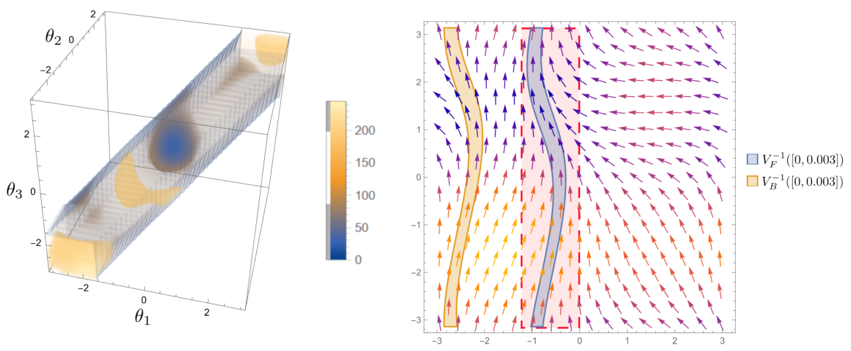
We similarly performed computations for system (38) of four oscillators with coupling function . Considering the corresponding phase-difference system obtained by substituting for , we obtained matrices , , and satisfying (35) for . This implies the existence of a local Lyapunov function in . The function is plotted in Figure 4, and the phase-difference system is locally stable in the region .
Recall that Theorem 1 and Remark 1 can be used to certify almost global phase-locking of nonuniform oscillators if the singularity of the obtained Lyapunov density for its phase-difference system is a singleton. We demonstrate it with the help of the following example.
Example 3
(Almost global phase-locking in three nonuniform coupled oscillators).
where , , , and . The corresponding phase-difference system is given by
which differ from (40) and (41) just by a constant. The corresponding Gram-matrices can thus be obtained from (42) and (43) by changing and , respectively. The system has equibrium points and . Checking the set of equalities (17) without the zero-sum condition on , the code returns a Hermitian matrix whose corresponding polynomial has a unique minimum approximately at according to Mathematica 13.2, where it assumes the value . Thus, it must imply that this point is a zero (approx.) of the function . As discussed in the introduction, such a point must exist since the density inevitably has a singularity [21]. Note that small errors arise due to approximations in numerical solutions. Thus, the phase-difference system exhibits almost global stability to the point . This implies that the original system (45) exhibits almost global phase-locking with and for almost all initial conditions.
In general systems, even more complex dynamics can be captured, such as the phase-cohesiveness of oscillators. An oscillator pair is phase-cohesive if there exists a constant and such that for all . A coupled system is said to be partially-phase-cohesive,28], for if there exists and such that for all .
Example 4.(Almost global partial-phase-cohesion in nonuniform Kuramoto model with a tree-topology: characterizing limit cycles) Consider a coupled nonuniform Kuramoto model (14) of three oscillators with topology , meaning , and coupling . Suppose , and , then using and , the corresponding phase difference is obtained as
The system does not have an equilibrium point. The code returns matrices and for and respectively, satisfying (17). These give rise to functions and , expressions in the Appendix, such that their reciprocals are Lyapunov densities for forward and backward flow, respectively, of the system . This implies that almost all solutions reach in backward time (hence it is a repellor) and reach in the forward time (hence it is an attractor), refer Figure (Figure 4) (right). Notice that almost all trajectories get trapped in the region . This implies that oscillators and eventually satisfy for almost all initial conditions. Hence, the system is almost globally phase-cohesive. Note that the existence of a Lyapunov density for systems with no equilibrium points will certify the presence of a limit cycle.
The reader might have realized that if it so happens that is the line , then almost all trajectories of the phase-difference system satisfy , which eventually implies that . Thus, the original system exhibits almost global (1,3)-phase synchronization. It should be noted if the system has multiple attractors, then the above process will inevitably fail. In such cases, if a point on the limit cycle is known, the code of local stability can be slightly modified to get a local characterization of the limit cycle. Gluing parts of the limit cycle obtained through this procedure could give a bigger picture, in theory, but it seems highly impractical. The methods in this article also extend to coupled oscillators, which depend on the collective interaction of more than two oscillators. For the interaction of three oscillators, these take the form
and are known to exhibit complex dynamics. We end this section by shedding light upon the fact that, due to phase-shift symmetry, all the methods and observations discussed via the preceding examples can be used as a framework to analyze the dynamics of coupled oscillators with higher-order coupling.
5. Conclusions
We develop a certification of almost global stability of the dynamical system on hypertorus using Gram matrix representation and trace parametrization of multivariate trigonometric polynomials in Theorem 1. We employ Theorem 1 to the system of all-to-all uniformly coupled oscillators of in Example 1. We obtain the parameters plane for certifying the almost global phase synchronization of the system in Figure 2. In Example 3, we obtain a Gram matrix to certify almost global phase-locking in three nonuniform coupled oscillators using Theorem 1. We also use Theorem 1 for almost global partial-phase-cohesion in a nonuniform Kuramoto model with a tree-topology in Example 4. Using Putinar’s Positivstellensatz Lemma 2, we construct a novel approach to certify the local Lyapunov stability on systems on hypertorus in Theorem 2. We apply this theory to certify local phase synchronization of uniform all-to-all coupled for three or four oscillators in Example 2 with local solutions Figure 3.
Appendix A
The expression of and in Example 4 is given by
References
- Tedrake, R.; Manchester, I.R.; Tobenkin, M.; Roberts, J.W. LQR-trees: Feedback motion planning via sums-of-squares verification. The International Journal of Robotics Research 2010, 29, 1038–1052. [CrossRef]
- Moore, J.; Tedrake, R. Control synthesis and verification for a perching UAV using LQR-Trees. 2012 IEEE 51st IEEE Conference on Decision and Control (CDC). IEEE, 2012, pp. 3707–3714. [CrossRef]
- Yoon, S.; Park, S.; Kim, Y. Circular motion guidance law for coordinated standoff tracking of a moving target. IEEE Transactions on Aerospace and Electronic Systems 2013, 49, 2440–2462.
- Liu, Z.; Zhang, Y.; Yu, X.; Yuan, C. Unmanned surface vehicles: An overview of developments and challenges. Annual Reviews in Control 2016, 41, 71–93. [CrossRef]
- Misra, R.; Wisniewski, R.; Karabacak, Ö. Sum-of-Squares based computation of a Lyapunov function for proving stability of a satellite with electromagnetic actuation. IFAC-PapersOnLine 2020, 53, 7380–7385. [CrossRef]
- Angeli, D. An almost global notion of input-to-state stability. IEEE Transactions on Automatic Control 2004, 49, 866–874. [CrossRef]
- Koditschek, D.E.; others. The application of total energy as a Lyapunov function for mechanical control systems. Dynamics and control of multibody systems 1989, 97, 131–157. [CrossRef]
- Rantzer, A. A dual to Lyapunov’s stability theorem. Systems & Control Letters 2001, 42, 161–168. [CrossRef]
- Prajna, S.; Parrilo, P.A.; Rantzer, A. Nonlinear control synthesis by convex optimization. IEEE Transactions on Automatic Control 2004, 49, 310–314. [CrossRef]
- Henrion, D.; Garulli, A. Positive polynomials in control; Vol. 312, Springer Science & Business Media, 2005.
- Dumitrescu, B. Positive trigonometric polynomials and signal processing applications; Vol. 103, Springer, 2007.
- Alkire, B.; Vandenberghe, L. Convex optimization problems involving finite autocorrelation sequences. Mathematical Programming 2002, 93, 331–359. [CrossRef]
- Davidson, T.N.; Luo, Z.Q.; Sturm, J.F. Linear matrix inequality formulation of spectral mask constraints with applications to FIR filter design. IEEE Transactions on Signal Processing 2002, 50, 2702–2715. [CrossRef]
- Zhang, J.H.; Janschek, K.; Böhme, J.; Zeng, Y.J. Multi-resolution dyadic wavelet denoising approach for extraction of visual evoked potentials in the brain. IEE Proceedings-Vision, Image and Signal Processing 2004, 151, 180–186. [CrossRef]
- Niemistö, R.; Dumitrescu, B.; Tăbuş, I. SDP design procedures for near-optimum IIR compaction filters. Signal processing 2002, 82, 911–924. [CrossRef]
- Henrion, D.; Vyhlídal, T. Positive trigonometric polynomials for strong stability of difference equations. IFAC Proceedings Volumes 2011, 44, 296–301. [CrossRef]
- Mayer, T. Polyhedral faces in Gram spectrahedra of binary forms. Linear Algebra and its Applications 2021, 608, 133–157. [CrossRef]
- McLean, J.W.; Woerdeman, H.J. Spectral factorizations and sums of squares representations via semidefinite programming. SIAM journal on matrix analysis and applications 2002, 23, 646–655. [CrossRef]
- Lee, J. Introduction to Smooth Manifolds; Graduate Texts in Mathematics, Springer New York, 2012.
- Kudeyt, M.; Kıvılcım, A.; Köksal-Ersöz, E.; İlhan, F.; Karabacak, Ö. Certification of almost global phase synchronization of all-to-all coupled phase oscillators. Chaos, Solitons & Fractals 2023, 174, 113838. [CrossRef]
- Karabacak, Ö.; Wisniewski, R.; Leth, J. On the almost global stability of invariant sets. 2018 European Control Conference (ECC). IEEE, 2018, pp. 1648–1653. [CrossRef]
- Ha, S.Y.; Ryoo, S.Y. Asymptotic phase-locking dynamics and critical coupling strength for the Kuramoto model. Communications in Mathematical Physics 2020, 377, 811–857. [CrossRef]
- Chopra, N.; Spong, M.W. On Exponential Synchronization of Kuramoto Oscillators. IEEE Transactions on Automatic Control 2009, 54, 353–357. doi:10.1109/TAC.2008.2007884. [CrossRef]
- Ha, S.Y.; Ha, T.; Kim, J.H. On the complete synchronization of the Kuramoto phase model. Physica D: Nonlinear Phenomena 2010, 239, 1692–1700. [CrossRef]
- Ashwin, P.; Burylko, O.; Maistrenko, Y. Bifurcation to heteroclinic cycles and sensitivity in three and four coupled phase oscillators. Physica D: Nonlinear Phenomena 2008, 237, 454–466. [CrossRef]
- Hansel, D.; Mato, G.; Meunier, C. Clustering and slow switching in globally coupled phase oscillators. Physical Review E 1993, 48, 3470. [CrossRef]
- Canale, E.; Monzón, P. Almost global synchronization of symmetric Kuramoto coupled oscillators. Systems Structure and Control 2008, 8, 167–190. [CrossRef]
- Qin, Y.; Kawano, Y.; Portoles, O.; Cao, M. Partial Phase Cohesiveness in Networks of Networks of Kuramoto Oscillators. IEEE Transactions on Automatic Control 2021, 66, 6100–6107. Conference Name: IEEE Transactions on Automatic Control, doi:10.1109/TAC.2021.3062005. [CrossRef]
Figure 1.
(Left) for and is a solid hexagonal cylinder as discussed in Remark 2; and (Right) appearing in the hypothesis of Corollary 3 for and .
Figure 1.
(Left) for and is a solid hexagonal cylinder as discussed in Remark 2; and (Right) appearing in the hypothesis of Corollary 3 for and .
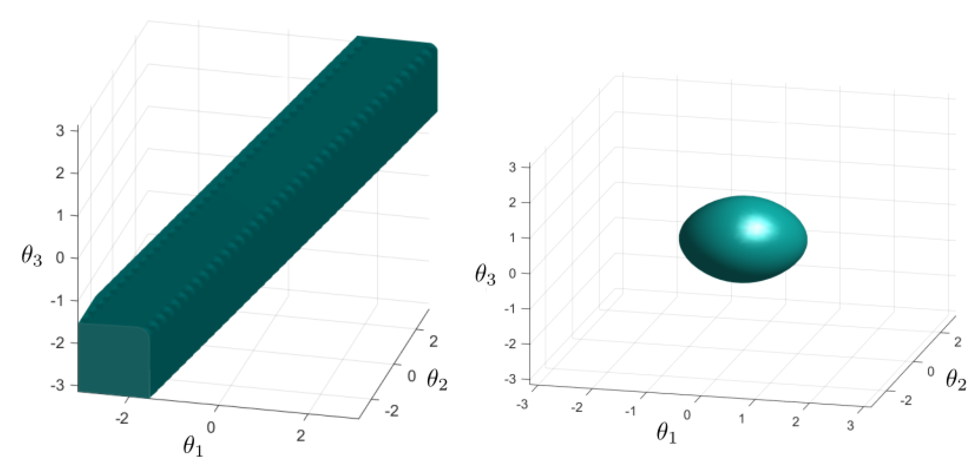
Figure 2.
Parameters for certifying almost global stability of (44) obtain by employing Theorem 1 and Gram matrices. Each blue star depicts a pair of parameter for which (44) is almost global phase synchronized. For each such pair, two positive semidefinite matrices and satisfying (17) exist and hence is a Lyapunov density due to Corollary 1 and Theorem 1.
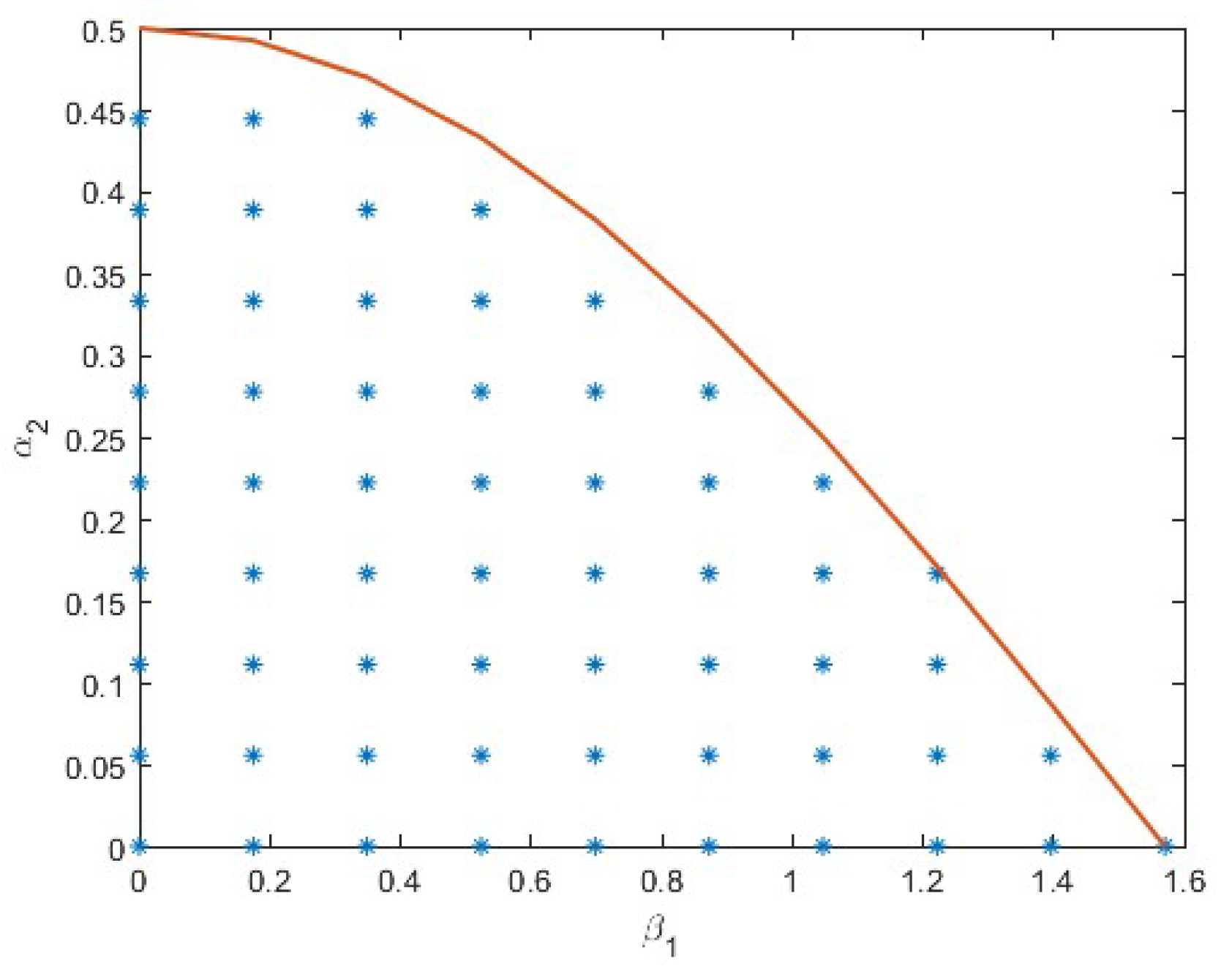
Figure 3.
(Left) flow and equilibrium points (red dots) of the phase-difference system (40)–(41); and several regions discussed in Example 2. The reduced vector field and the regions are obtained from their three-dimensional counterparts (right) on quotient-ing by the equivalence relation ∼ defined by if and only if for some .
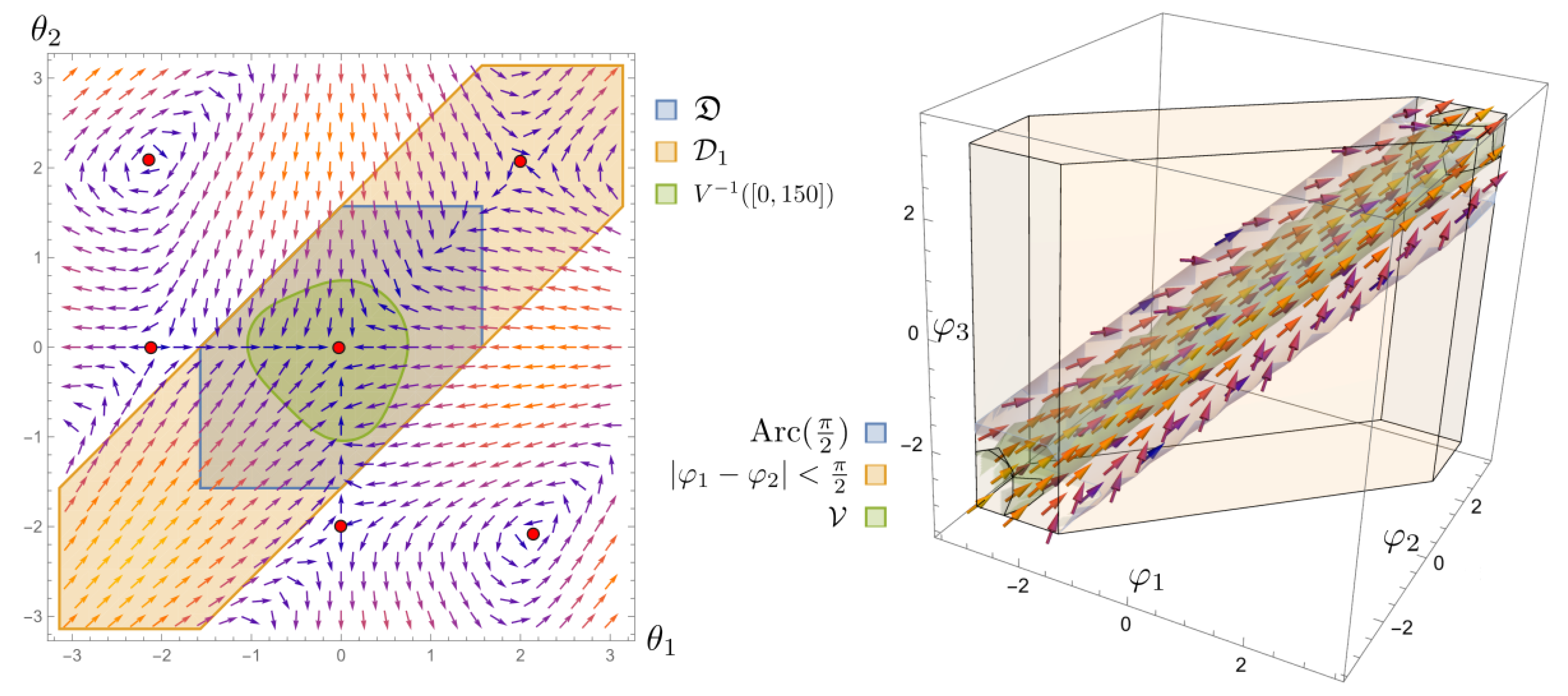
Figure 4.
(Left) The plot of Lyapunov function over in Example 2 implying that the all-to-all coupled uniform oscillators (38) for coupling (39) with and exhibit local synchronization. (Right) Verification that almost all solutions emerge from the repeller and reach the attractor for the phase-difference system in Example 4.
Disclaimer/Publisher’s Note: The statements, opinions and data contained in all publications are solely those of the individual author(s) and contributor(s) and not of MDPI and/or the editor(s). MDPI and/or the editor(s) disclaim responsibility for any injury to people or property resulting from any ideas, methods, instructions or products referred to in the content. |
© 2024 by the authors. Licensee MDPI, Basel, Switzerland. This article is an open access article distributed under the terms and conditions of the Creative Commons Attribution (CC BY) license (http://creativecommons.org/licenses/by/4.0/).
Copyright: This open access article is published under a Creative Commons CC BY 4.0 license, which permit the free download, distribution, and reuse, provided that the author and preprint are cited in any reuse.


