Feature Coding and Graph via Transformer: Different Granularities Classification for Aircrafts

1. Introduction

Identification and location of aircrafts are widely used and quite necessary in military, civilian unmanned clusters and navigation. Having a view of the future development on air vehicles and computer vision, there will be more needs in aircraft recognition in sky. Of course, convolutional neural network object detection algorithms, whether single-stage or multi-stage, training or inference, meets the most requirements of object localization and recognition. Although object detection focuses on multiple objects and classes from the early stages of its birth, the universal fine-grained classification models do not meet these recognition requirement, in which aircrafts are built and divided according to human design perspectives with a wide variety of similar types.

Classification aims at recognizing objects of various categories. Benefiting from convolutional neural networks, robust features make multi-class partitioning more precise. For classifying various objects in a certain category, which have no obvious dissimilarities, further requirements are needed. In the challenging task for recognizing similar sub-class aircrafts, even more detailed classes under finer classification criteria, higher requirements have been put forward for feature research due to the numerous subcategories and close appearance of aircrafts.

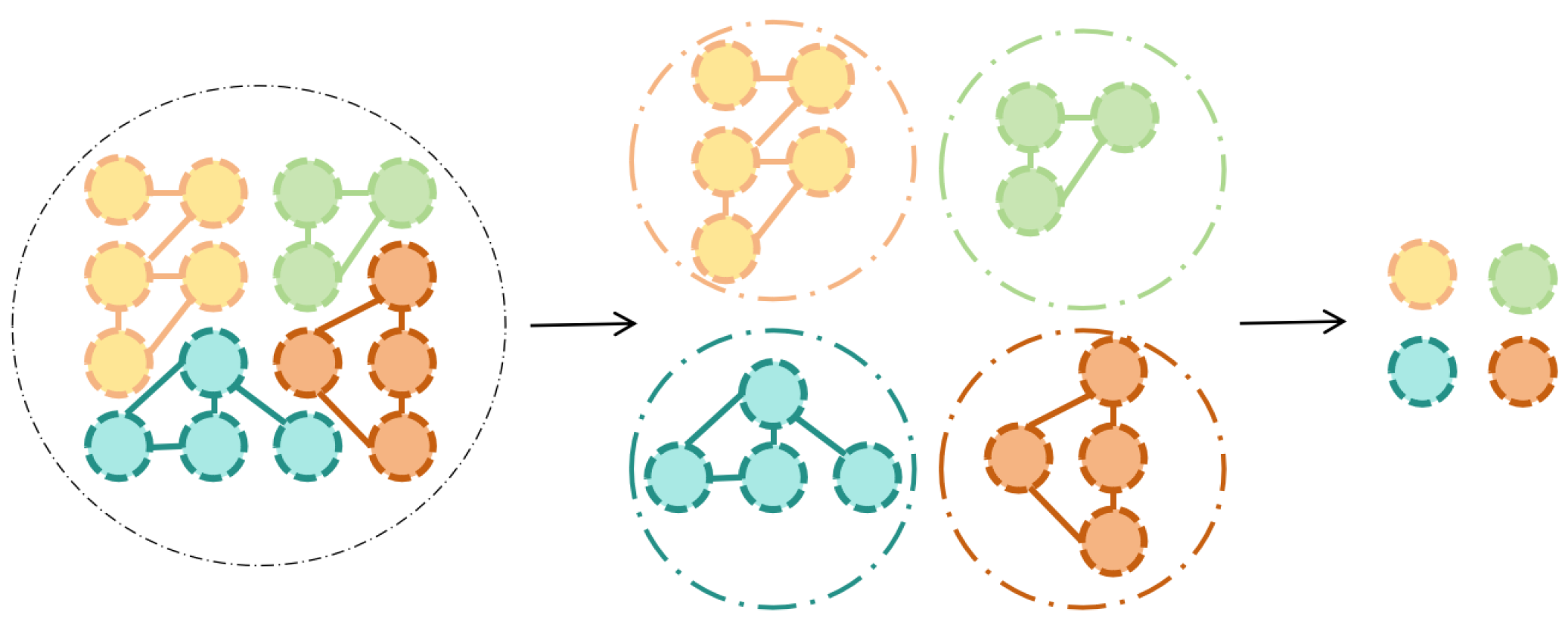
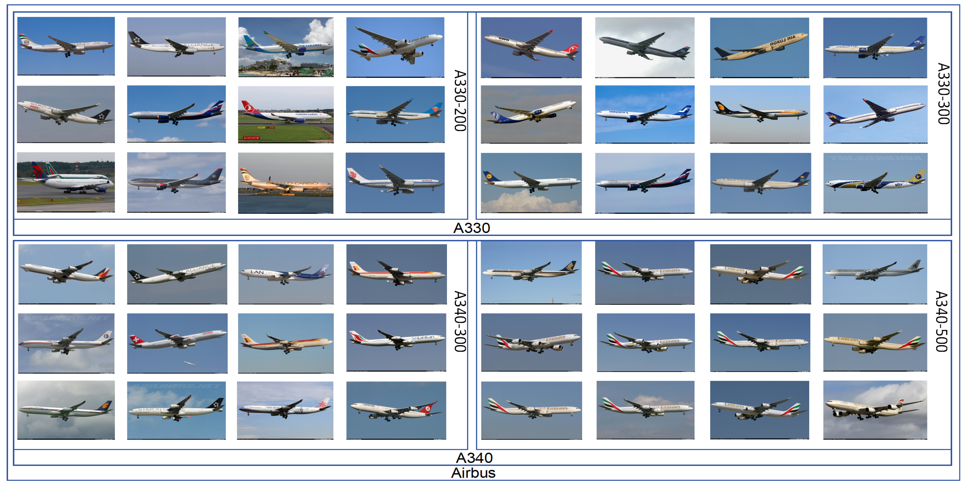
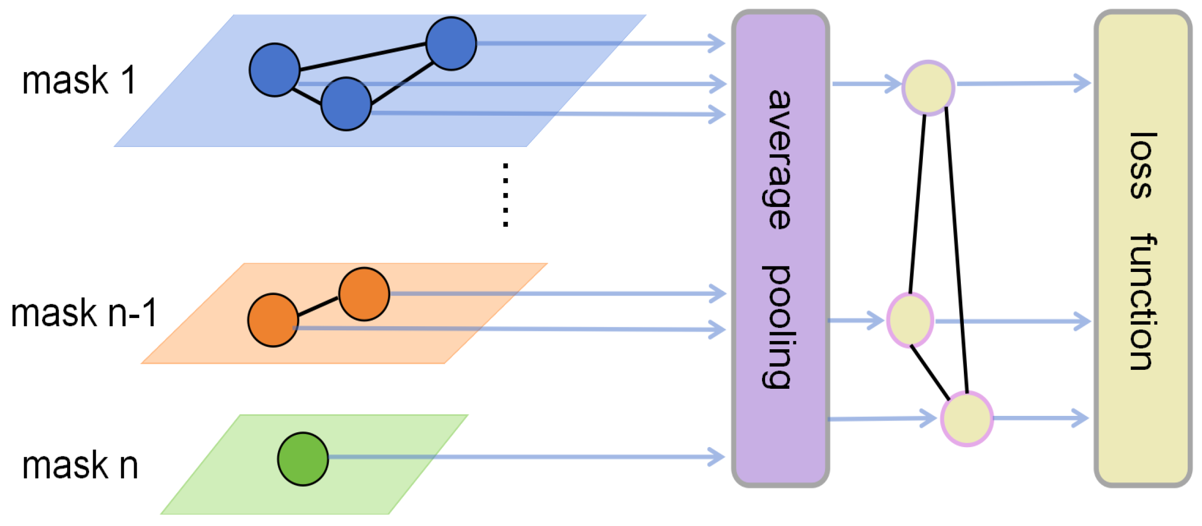
Figure 1. Data Partition of sample space under different criteria and labels in fine-grained classification

Figure 1. Data Partition of sample space under different criteria and labels in fine-grained classification

Coincidentally, fine-grained classification pay attention to deal such problems. In the development of fine-grained classification, algorithms [1–7] mainly follow two steps, one is locating an object, the other is classifying discriminative part features. As research deepens, Hu et al. [8] finds that holistic feature representation is important for fine-grained image classification. Moreover, Zhou et al.[9] proposed a self-supervised spatial context learning module, which aims at representing the holistic structure of objects. These are new ways comparing with approaches in the past.

However, there still are some complicated conditions, such as subcategories in the same basic category, which are unable to be resolved well. For aircrafts, research starts from the objective differences of rigid objects. The aircraft has a wide variety of categories, similar structures, and is based on artificial classification. Objects under these conditions may only be classified correctly with the help of some specific information.

In order to cope with these sophisticated application situations, the research of this paper, the fine-grained recognition of aircarfts, can be regarded as a further research in the application of fine-grained aircraft recognition, focusing on the sub-class identification in higher or more variable classification criteria.

Considering that general features extractions are extremely hard to distinguish quite similar objects from each other, it is suddenly spotted and paid attention to the relationship between image features and fine-grained classifications from other angles. In this paper, we seek to expand the applicability of Transformer such that it can serve as a solution for fine grained aircraft classification, given that it works for both NLP [10] and computer vision [11]. Its high performance in feature encoding and information representation to the visual domain caught our attention, and we decided to explore the relationships with fine-grained classification on aircrafts.

Thus, for both global information and features of aircraft parts, method we proposed considers these in Swin-T directly. We carried out research and experiments from the stage of tokens in swin-t, and ideas contain graph convolution are proposed to process the features. Furthermore, samples under different partitions artificially are fully observed and studied to explore the internal mechanism in our study.

Through extensive experimental verification, it has been proven that our feature processing method is effective in fine-grained aircraft recognition, whose classes and labels are splitted and divided artificially, and is superior to other algorithms and models for this task.

2. Background

2.1. Swin-Transformer [12]

The Transformer [13] architecture is a prevalent model design in natural language processing (NLP), specifically tailored for sequence modeling and transduction tasks. By integrating Query (Q), Key (K), and Value (V), which are generated by CNN to encoding the input information, and the model adeptly captures extensive dependencies from input information. The operation is accomplished within the feature space, and information in CNN is processed seamlessly across diverse regions of the feature space. In this kind of feature processing, Query operation extracts pertinent information, Key operation discerns crucial features, and the value operation assigns significance to these identified features. Collectively, these operations facilitate the establishment of a resilient and hierarchical representation. Furthermore, since the introduction of Vision Transformer (VIT) [14–17], numerous studies have continuously achieved substantial progress, which tailors the Transformer model for computer vision tasks. Among them [18,19], Swin Transformer establishes a hierarchical representation by commencing with smaller-sized patches, and progressively amalgamating adjacent patches in deeper layers of the Transformer.

2.2. Transformer and GNN

Transformer was first born and used in the field of natural language processing(NLP). the core idea of transformer is a kind of attention mechanism essentially. From the view of feature operation and calculation in transformer, attention distribution for tokens is calculated by encoder layers, and the attention scores weight the information of tokens.

In representation learning during the process of aggregating information, the long-term dependence within the sequence data shows marvelous effectiveness . Because of this, there are a number of existing works generalizing the transformer architecture to graph data in the level of feature maps.

In specific vision tasks, the design of node-wise positional encoding lack of analysis and comparison to subtle differences of data distribution. The specific form of coding, such as Laplacian encoding, positional encoding, has strong pertinence, but it is not suitable for the diversity of data.

Although there are existed calculation approach of graphs, such as Random Walk, having been studied both theoretically and empirically. The expensive calculation of pairwise attention does not suit the necessity of convenient and specific model fusion in vision tasks. ADSF 20 generats high order local receptive filed, and the GAT [21] is on the other side, furthermore, Coarformer [22] try to scale down and coarse the graph to apply the Transformer architecture, all of these are intended to be more adaptive to feature maps in models.

2.3. GNN and Classification

To various scales and isoetric graphs of input data, neural networks (GNNs)[23–34] which is based on graph adapts well. Considering about the diversity of data and vision tasks, GNN shows adaptability across common models.

The main differeces between GNN and other common models are that intricate geometric interrelationships in image datasets can be discerned by the extraction form of GNN, this is quite important to the predictive performance for objects who have the similar appearance but with different geometries.

We notice that GNNs are more and more adopted in X-ray imaging and medical imaging [35–41], including multi-modal data-based medical, essentially because of the ability of analysing complex interconnected phenomena. It has also been proven effective in human-object interaction detection and classification [42,43].

2.4. Fine-Grained Classification of Aircraft

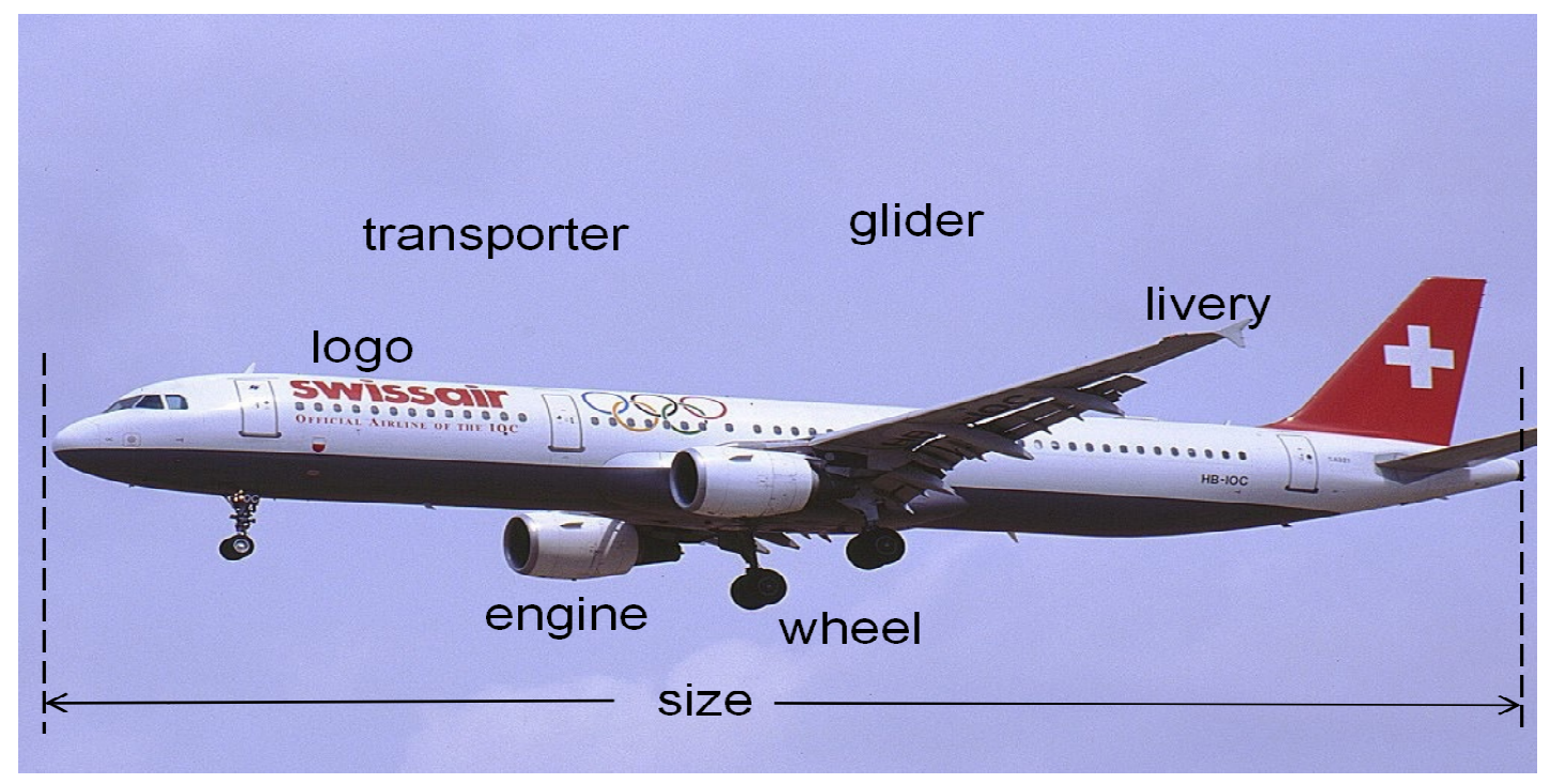
Aircraft, especially airplanes, are another sort of objects typically considered for fine-grained classification as cars and birds. In addition to a wide range of applications, there still are some factors which make aircraft recognition particularly interesting. Firstly, the design of aircraft spans a hundred years, during this period, many different models and hundreds of different makes and airlines came out. Secondly, aircraft designs vary significantly considering the size (from domestic aircraft carriers to large aircraft carriers), destination (military, private, civil), purpose (sport, fighter, carrier, transporter, training,etc.), propulsion (propeller, glider, jet), there are also other factors such as technology.In fact, the structure of the aircraft changes with their design (wheel per undercarriage, number of wings, engines, undercarriages, etc.)which is is not the same as categories such as animals [44–47]. Thirdly, any existed aircraft can be reused or repurposed by different companies, this may lead to the birth of further variations in appearance (livery). In recognition and classification task, we can consider this as noise. Finally, aircraft which are largely rigid objects remind us to focus on the core aspects of the fine-grained recognition problem, simplifying certain aspects in highly-deformable objects such as animals.

Figure 2. Features of aircraft in fine-grained classification

Figure 2. Features of aircraft in fine-grained classification

3. Materials and Methods

We aim to explore the fine use of DNN features and GNNs in transducing aircraft images into graphs. GNNs show strength in processing the transformed graph data, and were applied to classify images with subtle variations in features, such as pneumonia from medical images of the lungs.

Motivated by these features and advancements, in our study, we utilize the architecture of transformer to extract feature maps, and features are encoded in the process of network training.

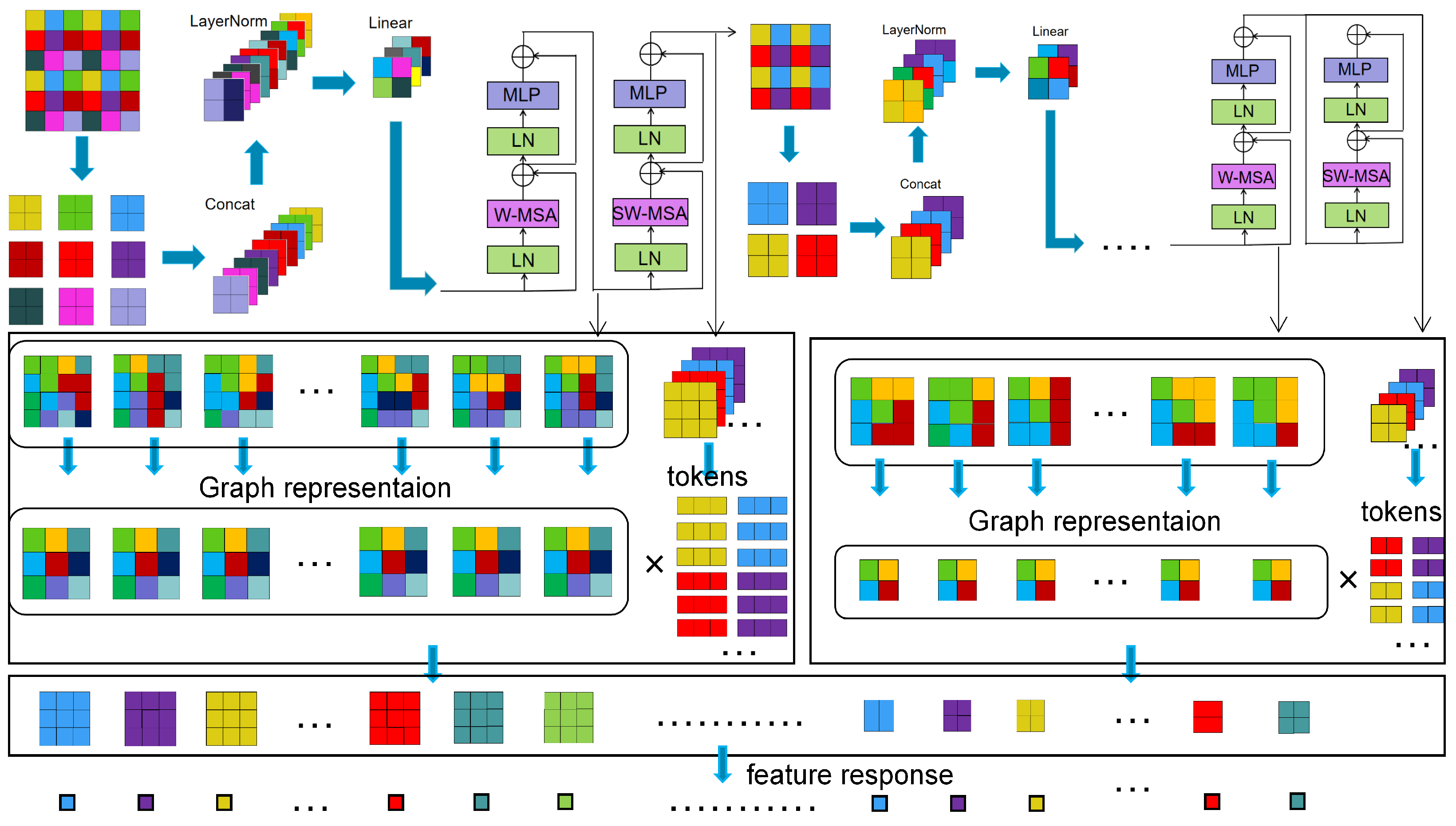
To leverage graph structure better for the fine grained classification task, our experiment design and conduction effectively include relevant features, which are captured both locally and globally. In order to explore the intrinsic mechanism of feature extraction in aircraft recognition tasks, and do research under different data partition criteria, we transform images into graphs. The graph structure not only enhances the representation, but also provides a more comprehensive understanding of the fine-grained aircraft differences. Our study analysis the relationship between the performance of classification and the nuances of data space partitioning, which reveals the relationship between subtle changes in data space and feature extraction. Based on coding and graph partitioning, improved performance is achieved through the use of feature computation.The overall flow and schematic diagram is shown below.

Figure 3. The overall flow and schematic diagram of the fine-grained aircraft classification

Figure 3. The overall flow and schematic diagram of the fine-grained aircraft classification

3.1. Feature Application in Swin-Transformer

1)graph representation for encoding information in transformer: In many graph representation learning scenarios, Graph Neural Networks (GNNs) have made great contribution which can be also considered for signals defined on graph structure data, such as feature maps of input images. Considering the same batch of data may be divided and mapped to various feature spaces, generalizing convolutional neural networks which bases on the theory of graph signal process can carry on more effective feature operation and calculation in essence.

While different filters are designed for graph signals, GNNs still suffer from much irrelevant information. Via CNN module, we can design different message passing mechanism which makes information aggregation more deep.

First, we extract feature maps at different semantic levels as graph data. We denote these layer as $H_i\in R^{N\times d_{in}}$, we define $h_i$ as the representation of central node $v_i$. If we choose n layers as graph data, we can concatenate them to get a new matrix $H\in R^{N\times n\times d_{in}}$:

$$H=Concat(H_1,\dots ,H_n)$$

(1)

As we know, graph convolution is a deep learning method for graph data. The usual calculation is shown as below for layer l, c is the coefficient, $\sigma (.)$ is non-linear transformation:

$$h_i^{l+1}=\sigma (\sum _{j\in v_i}{\displaystyle \frac{1}{c}}{h}_j^l{w}^l)$$

(2)

The whole calculation can be seen as operating at graph level and node level. For the graph data we get from neural network, we change the operation form of graph data to make it more effective, and study the problem we focused more deeply.

Figure 4. new nodes formed by weighting nodes in different regions at graph level and node level

Figure 4. new nodes formed by weighting nodes in different regions at graph level and node level

First we reform the structure of the graph data, and the pooling operation of data is realized at the same time. We adopt linear layer to soften sub-domain nodes with weighted situation. In the architecture of transformer, there are three matrices, $W_q$,$W_k$,$W_v$, which are used to represent q, K and V correspondingly.

$$q=h_i{W}_q$$

(3)

$$K=H{W}_k$$

(4)

$$V=H_i{W}_v$$

(5)

2)graph data correlation matrix multiplication:

To understand the contexts captured by attention, the tensors from different layers illustrate the information. The information corresponds to features extracted under different criteria. We could use the concept of word vectors to understand these feature information.

From the perspective of tensor calculation, tensor a multiply with a larger weight $w_{ij}$ , the i-th word in the source tensor pays more attention to the j-th word during the calculation of multiplication. The calculation result represents the attention maps which consists of two strong patterns: diagonal and sparse.

In the process of calculation, the sparse features stand for the long-term information, the correlation in small neighborhoods mostly appear in the diagonal. The relationship of various features in the same feature map can be simplified as “global” and “local”.

Figure 5. graph data correlation matrix multiplication

Figure 5. graph data correlation matrix multiplication

In our transformed graph structure $H_1$, one-dimensional convolution is performed to get $W_q$ and $W_k$. We average each row of the two matrixes so that they corresponds to tokens. At the node level, the graph structure is not changed, and only the signal of the graph is processed. We use one-dimension convolution to get graph data transformation, which also ensures the data volume maintains the same. So, we get the transformed graph data $H_2$, the matrix multiplication to complete the non-linear transformation is followed after this:

$$H_3=H_1{H}_2$$

(6)

3)classifier based on joints in graph data:

Similarly, we do batch-normalization on the results, meanwhile, the results of correlation by multiplying are the joints used for the later classification. The joints represent data response in the process of matrix multiplication, and in the process of training, they also represent the extraction of nuanced data information computation.

For these joints in various maps generated from graph data, we calculated the response values separately. Suppose $\left\{P_1^i,P_2^i\dots P_n^i\right\}$ is the set of joints for maps of channel i, we can calculate the final response value based on the data channel i.

$$R_i=Linear(P_1^i,P_2^i\dots P_n^i)$$

(7)

Figure 6. Joints generated from graph data and the final response

Figure 6. Joints generated from graph data and the final response

Along the same lines, we calculate the response values for all data channels. Then we get the response values set $\left\{R_1,R_2\dots R_i\right\}$. In the response values set, data represents the features response of input images, which are generated after feature coding and graph calculation in different channels. Finally, we send these feature response values to the classifier to get the final classification result.

$$I_{out}=Classifier(R_1,R_2\dots R_i)$$

(8)

3.2. The Process of Forward and Backward Propagation

Under different classification criteria, characteristics of semantic granularity vary in degree of detail. In order to make the numerical computation in neural network module capture the differences in subtlety. Aiming to perform fine-grined classification of aircrafts for various classification criteria, dataset under multi-variable classification criteria focus on dividing the sample space into various sub-space, which promotes different back-propagation gradient flows to be generated from the same inputs in supervised training.

While being trained, the features in feature maps present different degrees of discrimination ability to input data. Considering making full use of the discrimination ability from feature maps, we calculates all these features mentioned above in loss function. For feature map $f_i$, we can calculate the sum of the feature points in the map as:

$$l_i={\displaystyle \frac{1}{m\times n}}\sum _{x=1}^m\sum _{y=1}^n{I}_{x,y}$$

(9)

If we use the value of h maps as the criterion for classification, then the class loss is calculated through Cross Entropy, as shown below:

$$L_c=-\sum _{i=1}^{h}log\left(l_i^{cls}\right)$$

(10)

To reduce the negative effect of artificial data partition during network training, whose distribution space has a direct impact and influence on loss function, we design a buffer correction term for the loss function. The buffer correction term avoids selective judgment by the neural network, and selects out feature points with strong discrimination. S is a learnable mask tell whether feature is important or not.

$$I(x,y)=\left\{\begin{array}{c}I(x,y),if(x,y)\in S\hfill \\ 0,Otherwise\hfill \end{array}\right.$$

(11)

Figure 7. Loss function calculation

Figure 7. Loss function calculation

Combine the above two expressions and bring in the features in S, then we can calculate the loss function as follows.

$$L_s=-\sum _{i=1}^{h}log(({\displaystyle \frac{1}{m\times n}}\sum _{x=1}^m\sum _{y=1}^n{I}_{out}{)}^{cls})$$

(12)

4. Experiments

In this section, we introduce the dataset that was partitioned under various criteria, the corresponding relationship between data samples and categories under these criteria.

These different partitioned datasets are used for training and compared. We then describe the various experiments that were conducted for training different encoding and graph feature calculation approaches. Experiment results and processing are compared and analysised to reveal the essence we discussed in fine-grained aircraft classification.

4.1. Datasets and Various Artificial Labeling Criteria

FGVC-Aircraft contains 10000 images and spans 100 categories of aircraft. Based on multi-variable classification criteria, the dataset has been organised in a three-level hierarchy, which contains aircrafts of 100 variants grouped under 70 families and 30 manufacturers respectively.

This dataset adopts the most specific class label. In the same model of aircraft, from the exterior of aircraft in the given images, we can find that differences between aircrafts may not be visually measurable.

• Classification Criterion 1: In this level,after merging visually indistinguishable aircraft models, we dived dataset into various model variants whose finer distinctions are visually detectable.
• Classification Criterion 2: Model variants that differ in subtle ways in criteria 1 are grouped together into families, making differences among each class more substantial, which creates a classification task of intermediate difficulty.
• Classification Criterion 3: On the basis of the criterion 2, we classify the products produced by the same manufacturer into the same category.

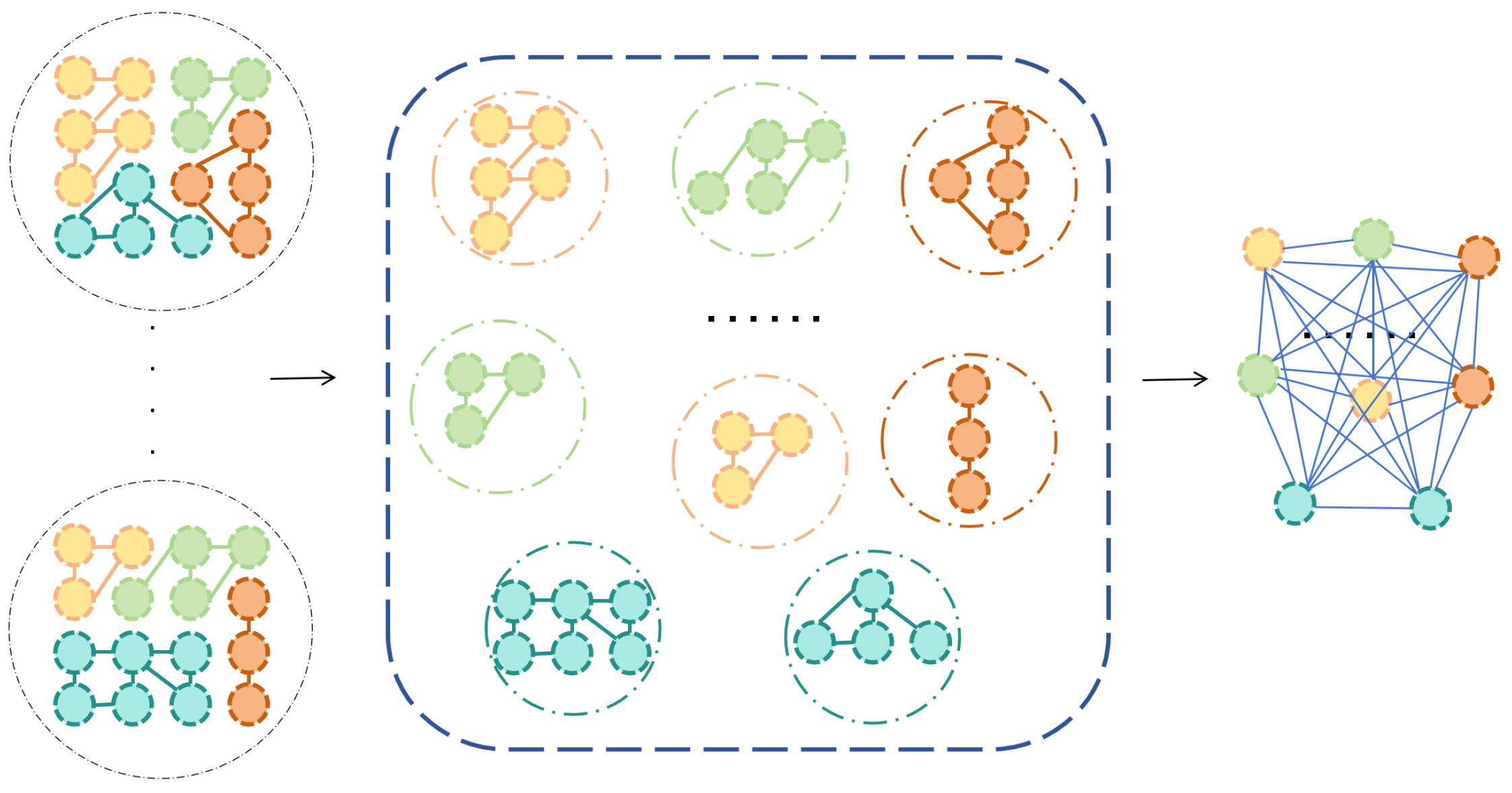
The detailed grouping, labeling and their affiliation are shown in the table. Under theses classification criteria, data are still prepared as training data and test data, which can be used to verify the prediction ability of the neural network structure for aircraft fine-grained classification under different data space partition.

Figure 8. Class labels for the same data under different classification criteria

Figure 8. Class labels for the same data under different classification criteria

Table 1. The relationship of labels under various division criteria-1.

Manufacture	Family	Variant
Airbus	A300	A300B4
	A310	A310
	A320	A318
		A319
		A320
		A321
	A330	A330-200
		A330-300
	A340	A340-200
		A340-300
		A340-500
		A340-600
	A380	A380
Manufacture	Family	Variant
Antonov	An-12	An-12
ATR	ATR-42	ATR-42
	ATR-72	ATR-72
British Aerospace	BAE	BAE
	BAE-125	BAE-125
Beechcraft	Beechcraft	Beechcraft
Douglas Aircraft Company	C-47	C-47
Lockheed Corporation	C-130	C-130
Cessna	Cessna	Cessna
Canadair	Challenger	Challenger
	CRJ-200	CRJ-200
	CRJ-700	CRJ-700
		CRG-900

Table 1. The relationship of labels under various division criteria-1.

Manufacture	Family	Variant
Airbus	A300	A300B4
	A310	A310
	A320	A318
		A319
		A320
		A321
	A330	A330-200
		A330-300
	A340	A340-200
		A340-300
		A340-500
		A340-600
	A380	A380
Manufacture	Family	Variant
Antonov	An-12	An-12
ATR	ATR-42	ATR-42
	ATR-72	ATR-72
British Aerospace	BAE	BAE
	BAE-125	BAE-125
Beechcraft	Beechcraft	Beechcraft
Douglas Aircraft Company	C-47	C-47
Lockheed Corporation	C-130	C-130
Cessna	Cessna	Cessna
Canadair	Challenger	Challenger
	CRJ-200	CRJ-200
	CRJ-700	CRJ-700
		CRG-900

Table 2. The relationship of labels under various division criteria-2.

Manufacture	Family	Variant
Boeing	Boeing 707	707-320
	Boeing 727	727-200
	Boeing 737	737-200
		737-300
		737-400
		737-500
		737-600
		737-700
		737-800
		737-900
	Boeing 747	747-100
		747-200
		747-300
		747-400
	Boeing 757	757-200
		757-300
	Boeing 767	767-200
		767-300
		767-400
	Boeing 777	777-200
		777-300
	Boeing 717	717
Douglas Aircraft Company	DC-3	DC-3
	DC-6	DC-6
	DC-8	DC-8
McDonnell Douglas	DC-9	DC-9-30
	DC-10	DC-10
	MD-11	MD-11
	MD-80	MD-80
		MD-87
	MD-90	MD-90
	F	F

Table 2. The relationship of labels under various division criteria-2.

Manufacture	Family	Variant
Boeing	Boeing 707	707-320
	Boeing 727	727-200
	Boeing 737	737-200
		737-300
		737-400
		737-500
		737-600
		737-700
		737-800
		737-900
	Boeing 747	747-100
		747-200
		747-300
		747-400
	Boeing 757	757-200
		757-300
	Boeing 767	767-200
		767-300
		767-400
	Boeing 777	777-200
		777-300
	Boeing 717	717
Douglas Aircraft Company	DC-3	DC-3
	DC-6	DC-6
	DC-8	DC-8
McDonnell Douglas	DC-9	DC-9-30
	DC-10	DC-10
	MD-11	MD-11
	MD-80	MD-80
		MD-87
	MD-90	MD-90
	F	F

Table 3. The relationship of labels under various division criteria-3

Manufacture	Family	Variant
Eurofighter	Eurofighter	Eurofighter
Lockheed Martin	F-16	F-16A
Dassault Aviation	Falcon	Falcon
Fokker	Fokker	Fokker
Bombardier Aerospace	Global	Global
Gulfstream Aerospace	Gulfstream	Gulfstream
British Aerospace	Hawk	Hawk
Ilyushin	Il-76	Il-76
Lockheed Corporation	L-1011	L-1011
Fairchild	Metroliner	Metroliner
Beechcraft	King Air	Model
Piper	PA-28	PA-28
Saab	Saab	Saab
Supermarine	Spitfire	Spitfire
Cirrus Aircraft	SR-20	SR-20
Panavia	Tornado	Tornado
Tupolev	Tu-134	Tu-134
	Tu-154	Tu-154
Yakovlev	Yak-42	Yak-42
de Havilland	DH-82	DH-82
	DHC-1	DHC-1
	DHC-6	DHC-6
	Dash 8	DHC-8-100
		DHC-8-300
Manufacture	Family	Variant
Dornier	Dornier	Dornier
Robin	DR-400	DR-400
Embraer	Embraer E	E-170
		E-190
		E-195
	EMB-120	EMB-120
	Embraer	Embraer
	ERJ	ERJ

Table 3. The relationship of labels under various division criteria-3

Manufacture	Family	Variant
Eurofighter	Eurofighter	Eurofighter
Lockheed Martin	F-16	F-16A
Dassault Aviation	Falcon	Falcon
Fokker	Fokker	Fokker
Bombardier Aerospace	Global	Global
Gulfstream Aerospace	Gulfstream	Gulfstream
British Aerospace	Hawk	Hawk
Ilyushin	Il-76	Il-76
Lockheed Corporation	L-1011	L-1011
Fairchild	Metroliner	Metroliner
Beechcraft	King Air	Model
Piper	PA-28	PA-28
Saab	Saab	Saab
Supermarine	Spitfire	Spitfire
Cirrus Aircraft	SR-20	SR-20
Panavia	Tornado	Tornado
Tupolev	Tu-134	Tu-134
	Tu-154	Tu-154
Yakovlev	Yak-42	Yak-42
de Havilland	DH-82	DH-82
	DHC-1	DHC-1
	DHC-6	DHC-6
	Dash 8	DHC-8-100
		DHC-8-300
Manufacture	Family	Variant
Dornier	Dornier	Dornier
Robin	DR-400	DR-400
Embraer	Embraer E	E-170
		E-190
		E-195
	EMB-120	EMB-120
	Embraer	Embraer
	ERJ	ERJ

4.2. Implementation Details

In our experiments, Swin-T which has four blocks is used as the backbone.

The Swim-T model is a four-stage hierarchical Transformer that integrates window multi-head self-attention (W-MSA) and shifted-window multi-head self-attention (SW-MSA) layers. Specifically, the Swin-T model contains four stages and each stage has a different number of Swin-Transformer blocks. The image is first divided into non-overlapping patches and then fed into stage one with two Swin-Transformer blocks. Through this process, the original image with dimension of H × W × 3 is transformed into the feature map with dimension of H/4×W/4×C. Subsequently, the second to fourth stages of the Swim-T model consist of two, six and two Swin-Transformer blocks, respectively. While augmenting the number of channels, these stages are designed to decrease the size of feature maps and acquire feature representation.

During the process of training, cosine decay is adopted, the parameter weight decay is set to 0.0005; the optimizer is chosen as SGD, and the batch size is set to 16. A total of 50 epochs are trained. All experiments are completed on a single Nvidia GeForce RTX 3090, and the Pytorch toolbox is used as the main implementation substrate. It takes about 1 hours to complete the training.

In training phrase, data augmentation is performed via Random HorizontalFlip,Randon Crop, and Random GaussianBlur. Center Crop is used in testing phrase. During training, the learning rate is set to 0.0005.

4.3. Evaluation Metrics

We can calculate the accuracy of the model by the following formula:

$$Accuray={\displaystyle \frac{TP+TN}{TP+TN+FP+FN}}$$

(13)

In the above formula, TP stands for true positive samples, FN stands for false negtive samples, FP stands for false positive samples, and TN stands for true positive samples.

4.4. Ablation Study and Analysis

4.4.1. Ablation Studies

We conduct an experiment to analysis and verify the ability of our model in the task, and show the various results with the different sample partitions of data. We used the data feature extraction and token encoding of transformer to get the query q and key k. We reshape q and k to get row vector of query and column vector of key. Then, matrix multiplication of theses two vectors is done directly, without the processing of our graph representation. We get a feature representation map in the architecture of transformer, and the later processing is to send feature representation map to get feature response values. We used the linear layer to get the final classification result. The experiment results in various data partition criteria are shown in the table. It is not difficult to find that the more finely divided the data are, the more difficult to obtain good performance of fine-grained aircraft classification.

1)graphic representation:This experiment is designed to verify the role of encoded data processing of transformer in our vision task. Compared with the experiment above, we get the graph data from feature map of $H_s$. Except query Q and key K, V for value can be calculated. We calculate the matrix A as follows:

$$A=tanh({\displaystyle \frac{Q-K}{v}})$$

(14)

2)graph data correlation matrix multiplication:Then we multiply $H_s$ and A by matrices, to avoid the calculation of A being too small, a diagonal matrix is added to the variable A at initialization time. The fine-grained classification performances are shown in the table.

3)classifier based on joints in graph data:By doing the differential processing of the coded information, differences are compared corresponding under various data partition. We can see that the performances are significantly improved in both Criteria 2 and Critetia 3.

4)classifier based on joints in graph data: In this experiment, we use another way to handle the mapping of coded information between Q and K. Instead of doing the difference(the coding information differences are mapped out by a non-linear function) and normalization simply, we take the method of correlation matrix multiplication proposed on graph data. The performance has been significantly improved under Criterion 3.

It is conducted to using the buffer correction term mentioned above. From the table which shows the performances of fine-grained classification. we can find that the approach has a more significant improvement for fine-grained classification under criterion 2.

Table 4. Ablation study

Method usage					Accuracy
$\left(\mathbf{1}\right)$	$\left(\mathbf{2}\right)$	$\left(\mathbf{3}\right)$	$\left(\mathbf{4}\right)$		$\mathbf{Criteria}\mathbf{1}$	$\mathbf{Criteria}\mathbf{2}$	$\mathbf{Criteria}\mathbf{3}$
✓					94.329	88.830	76.952
✓	✓				94.629	91.146	77.632
✓	✓	✓			94.629	92.544	80.572
✓		✓	✓		94.689	89.340	75.000
✓	✓	✓	✓		94.779	97.727	80.645

Table 4. Ablation study

Method usage					Accuracy
$\left(\mathbf{1}\right)$	$\left(\mathbf{2}\right)$	$\left(\mathbf{3}\right)$	$\left(\mathbf{4}\right)$		$\mathbf{Criteria}\mathbf{1}$	$\mathbf{Criteria}\mathbf{2}$	$\mathbf{Criteria}\mathbf{3}$
✓					94.329	88.830	76.952
✓	✓				94.629	91.146	77.632
✓	✓	✓			94.629	92.544	80.572
✓		✓	✓		94.689	89.340	75.000
✓	✓	✓	✓		94.779	97.727	80.645

In our ablation study, the buffer correction term improves the performance a lot under criteria 2. In this case, we remove the operation of correlation matrix multiplication, we can see the results in the table below.

This shows that, only learn freely through gradient descent without any other constraints, not considering feature operations of the data partition space, can not improve the performances. On contrary, correlation matrix multiplication is used in feature processing. Considering feature operations of the data partition space and without extra specific controlling of loss function, the performances on this task are not the same, which will be slightly better than the previous one.

So, artificial will can not be used to identify the characteristic representation of distinctions very well, the processing of feature coding and graph data play an important role.

4.4.2. Further Study of Information Encoding to Various data partition criteria

In ablation study, these experiments we conducted show that graph-based feature data processing can be effectively combined with transformation feature coding, which play a significant role in fine-grained classification of aircraft, especially when data is partitioned more and more finely. In the process of training gradient back-propagation, the subtle difference feature trained enough has a positive promoting effect on this task.

However, for different samples partition criteria, it is obvious that the performance of these methods and measures is not consistent. This reveals that, in the fine-grained classification of aircraft, general or pan-task learning does not perform well.

For information encoding, in addition to the standard calculation of Formula 14, we designed and compared a series of experiments for each data partition criterion. Then we analysis the performances of methods under different data partition criteria, so that we have a further study for the relationship between input data space partition and information of feature representation.We can find that making the difference of encoding information in transformer is the main factor of impelling our model to distinguish the differences.

Feature coding and graphical representation are essentially representations of the input information space, and we can see how they represent for the fine-grained classification of aircraft from various partition criteria. So we designed six more experiments to explore the specific situations.

(1)In this experiment, we multiply the Q and K convoluted from the graph-represented feature graph, Q transpose and do matrix multiplication with transpose, a response matrix of Q and K is obtained.the calculation method graph data correlation matrix multiplication mentioned in this paper is continued, response matrix and the graphic feature Hs mentioned above participate in the calculation. The classifier is based on the joints in graph data we proposed.

(2)The experimental design is basically the same as the previous one, except that we add a diagonal matrix to the response matrix of Q and K when it do correlation matrix multiplication with Hs.

(3)The difference between this experiment and the first one is that we use softmax to map the corresponding matrix of K and Q, this makes it possible to judge the feature information by category probability correlation when doing the graph data correlation matrix multiplication with Hs.

(4)The difference between this experiment and the first one is that we do not compute the response matrix of Q and K, we simply calculated the difference between Q and K instead. Suppose Q and k are row vectors with n elements, we use n vectors of Q and K, the calculation is as follows:

$$(Q^T,\dots Q^T)-{(K^T,\dots K^T)}^T$$

(15)

(5)The difference between this experiment and the forth one is that we used the buffer correction term we proposed.

(6)In this experiment, we abandoned the use of the encoding information of Q and K, we use the graph representation of features in transformer directly, the classifier is based on the joints in graph data, the buffer correction term is used.

Table 5. accuracy on various sample partitions.

Method	(1)	(2)	(3)	(4)	(5)	(6)
Criteria 1	94.659	94.569	94.869	95.080	94.419	94.689
Criteria 2	92.204	94.737	91.255	93.750	92.230	89.340
Criteria 3	81.250	79.051	77.619	72.699	82.168	75.000

Table 5. accuracy on various sample partitions.

Method	(1)	(2)	(3)	(4)	(5)	(6)
Criteria 1	94.659	94.569	94.869	95.080	94.419	94.689
Criteria 2	92.204	94.737	91.255	93.750	92.230	89.340
Criteria 3	81.250	79.051	77.619	72.699	82.168	75.000

The table shows the requirement of feature representation is higher with the finer subdivision of sample space. When the feature space is roughly divided, the distinct computation of coding information and graph representation of data can classify finer features well.

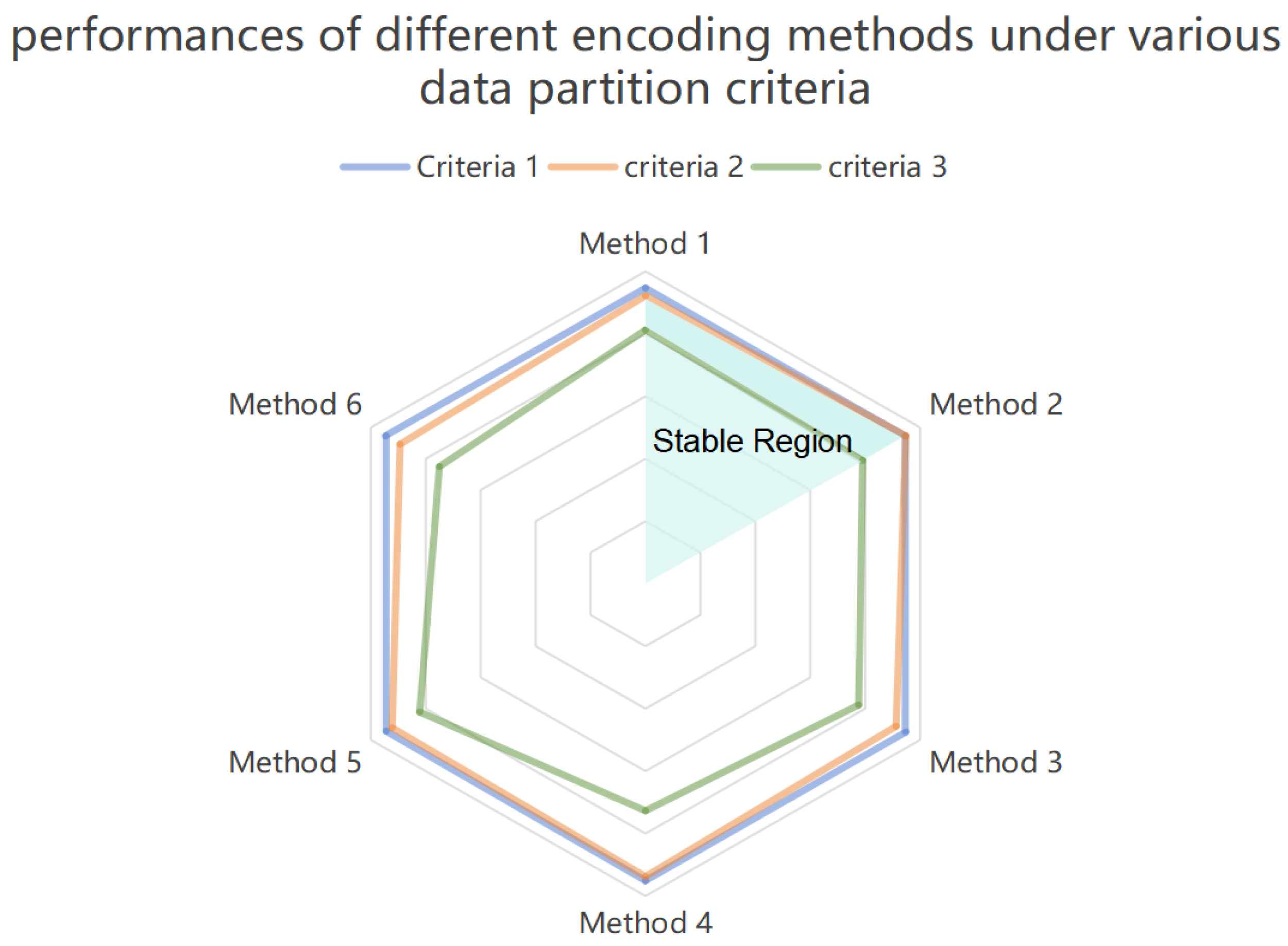
Figure 9. Further Study of Information Encoding to Various data partition criteria

Figure 9. Further Study of Information Encoding to Various data partition criteria

The figure above shows the effectiveness of various information encoding methods to values from transformer. When the subdivision of the sample space is finer, the difference comparison of the coding information is required to be more distinguished for classification. Compared with the response matrix, the subdivision of the sample space tell the distinguishing features in the subdivision of the more finer sample space. The closer the sample space is, the closer the input data is in the feature space. Meanwhile, the representation of coded information will be more important if the sample space is not divided sufficiently, and the gradient flow during training is not easy to affect the representation of these fine features. For the stably classification under various data partition criteria, the further analysis and figure above show that, full rank matrix and the linear variation of the superposition diagonal matrix is robust, other ways of encoding are sensitive to how the data is divided.

4.4.3. Comparison with other famous models

We also chose classic and efficient open source models in the field of fine-grained recognition, and test performances under different data partition criteria comparing with our approach. In general, the more subcategories you have, the more difficult it is to accurately identify, while artificial subcategories can also be slightly disruptive to models sometimes. Our approach shows excellent performance processing under different classification criteria, and achieves excellent accuracy of recognition via different feature encoding approaches. The performances are shown in the table below.

Table 6. Performances of various fine-grained classification models.

Fine-grained classification model	Accuracy
	$\mathbf{Criteria}\mathbf{1}$	$\mathbf{Criteria}\mathbf{2}$	$\mathbf{Criteria}\mathbf{3}$
NTS-Net	92.643	92.217	81.626
API-Net	79.922	71.939	53.463
DFL	78.848	84.338	74.017
FGVC	94.659	92.173	75.032
Bilinear-cnn	86.169	84.638	72.067
ours1	95.080	93.750	72.699
ours2	94.419	92.230	82.168
ours3	94.779	97.727	80.645

It represents the convolution layer of neural networks. The layer computes the result using convolution kernels by moving on a certain stride. The numbers of layers filled with 0 elements at the edge of the feature map are shown in the column of Padding

Table 6. Performances of various fine-grained classification models.

Fine-grained classification model	Accuracy
	$\mathbf{Criteria}\mathbf{1}$	$\mathbf{Criteria}\mathbf{2}$	$\mathbf{Criteria}\mathbf{3}$
NTS-Net	92.643	92.217	81.626
API-Net	79.922	71.939	53.463
DFL	78.848	84.338	74.017
FGVC	94.659	92.173	75.032
Bilinear-cnn	86.169	84.638	72.067
ours1	95.080	93.750	72.699
ours2	94.419	92.230	82.168
ours3	94.779	97.727	80.645

It represents the convolution layer of neural networks. The layer computes the result using convolution kernels by moving on a certain stride. The numbers of layers filled with 0 elements at the edge of the feature map are shown in the column of Padding

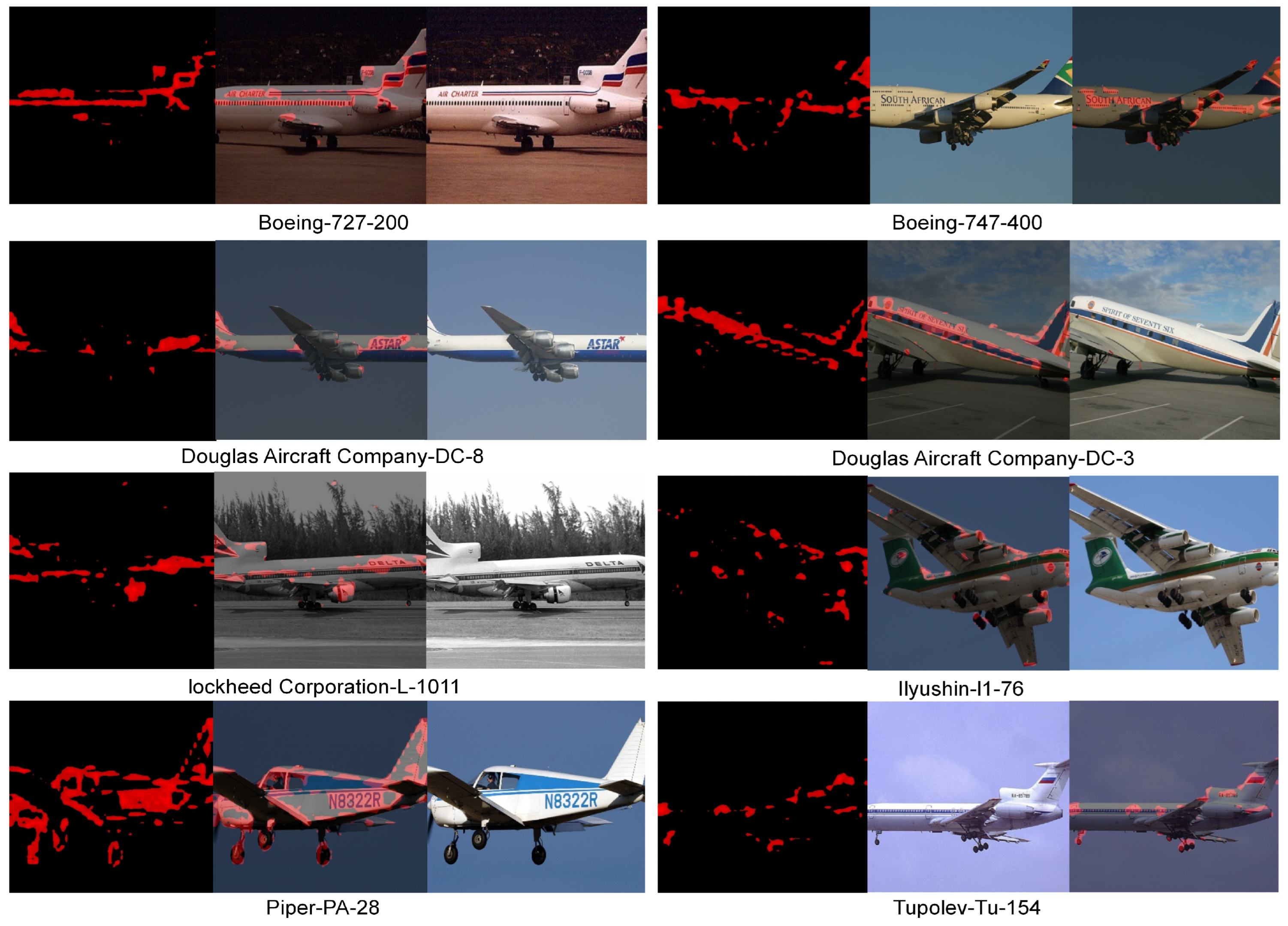
Figure 10. Heatmaps of our proposed approach in the process of input inference

Figure 10. Heatmaps of our proposed approach in the process of input inference

5. Conclusions

Our Paper demonstrates an innovate graph convolution representation and information encoding from Transformer for fine-grained aircraft classification. The graphic feature maps can enhance the classification performance with the help of transformer, which takes the subtlety of feature representation to a new level. Through the further study of the whole classification pipeline and a lot of experimental data, we proved that this way of encoding and information extraction can play a more positive role in the fine-grained classification of aircraft, which are artificial objects categorized by various man-made criteria. Meanwhile, we find that various representations of coded information are more attribute-oriented for different data partition criteria, which shows that task-oriented and man-made classification criteria, the fine-grained classification problems for special large classes of objects, can be guided by these after further study to some extent.

References

- A. Dosovitskiy, L. A. Dosovitskiy, L. Beyer, A. Kolesnikov, D. Weissenborn, X. Zhai, T. Unterthiner, M. Dehghani, M. Minderer, G. Heigold, S. Gelly, J. Uszkoreit, and N. Houlsby, "An image is worth 16x16 words: Transformers for image recognition at scale." in International Conference on Learning Representations, 2021. [CrossRef]
- Y. Ding, Y. Y. Ding, Y. Zhou, Y. Zhu, Q. Ye, and J. Jiao, “Selective sparse sampling for fine-grained image recognition,” in Proc. IEEE/CVF Int. Conf. Comput. Vision, 2019, pp. 6598–6607. [CrossRef]
- J. Fu, H. J. Fu, H. Zheng, and T. Mei, “Look closer to see better: Recurrent attention convolutional neural network for fine-grained image recognition,” in Proc. IEEE Conf. Comput. Vision Pattern Recognit., 2017, pp. 4476–4484. [CrossRef]
- C. Liu, H. C. Liu, H. Xie, Z.-J. Zha, L. Ma, L. Yu, and Y. Zhang, “Filtration and distillation: Enhancing region attention for fine-grained visual categorization,” in Proc. AAAI Conf. Artif. Intell., vol. 34, 2020, pp. 11555–11562. [CrossRef]
- Y. Peng, X. Y. Peng, X. He, and J. Zhao, “Object-part attention model for fine-grained image classification,” IEEE Trans. Image Process., vol. 27, no. 3, pp. 1487–1500, Mar. 2018. [CrossRef]
- N. Zhang, J. N. Zhang, J. Donahue, R. Girshick, and T. Darrell, “Part-based R-CNNs for fine-grained category detection,” in Proc. Eur. Conf. Comput. Vision, 2014, pp. 834–849. [CrossRef]
- X. Zhang, H. X. Zhang, H. Xiong, W. Zhou, and Q. Tian, “Fused one-vs-all features with semantic alignments for fine-grained visual categorization,” IEEE Trans. Image Process., vol. 25, no. 2, pp. 878–892, Feb. 2016. [CrossRef]
- H. Zheng, J. H. Zheng, J. Fu, Z.-J. Zha, and J. Luo, “Looking for the devil in the details: Learning trilinear attention sampling network for fine-grained image recognition,” in Proc. IEEE/CVF Conf. Comput. Vision Pattern Recognit., 2019, pp. 5007–5016. [CrossRef]
- Y. Hu, Y. Y. Hu, Y. Yang, J. Zhang, X. Cao, and X. Zhen, “Attentional kernel encoding networks for fine-grained visual categorization,” IEEE Trans. Circuits Syst. Video Technol., vol. 31, no. 1, pp. 301–314, Jan. 2021. [CrossRef]
- M. Zhou, Y. M. Zhou, Y. Bai, W. Zhang, T. Zhao, and T. Mei, “Look-into-object: Self-supervised structure modeling for object recognition,” in Proc. IEEE/CVF Conf. Comput. Vision Pattern Recognit., 2020, pp. 11771–11780. [CrossRef]
- Nuo Chen, Fenglin Liu, Chenyu You, Peilin Zhou, and Yuexian Zou. 2021. Adaptive bi-directional attention: Exploring multi-granularity representations for machine reading comprehension. In ICASSP 2021-2021 IEEE International Conference on Acoustics, Speech and Signal Processing (ICASSP). IEEE, 7833–7837. [CrossRef]
- Peiyan Zhang, Haoyang Liu, Chaozhuo Li, Xing Xie, Sunqhun Kim, and Hao han Wang. 2023. Foundation Model-oriented Robustness: Robust Image Model Evaluation with Pretrained Models. arXiv:2308.10632. [CrossRef]
- Z. Liu, Y. Z. Liu, Y. Lin, Y. Cao, H. Hu, Y. Wei, Z. Zhang, S. Lin, and B. Guo, “Swin transformer: Hierarchical vision transformer using shifted windows,” in Proceedings of the IEEE/CVF International Conference on Computer Vision (ICCV), pp. 10012–10022, 21. 20 October. [CrossRef]
- Ashish Vaswani, Noam Shazeer, Niki Parmar, Jakob Uszkoreit, Llion Jones, Aidan N. Gomez, Lukasz Kaiser, and Illia Polosukhin. 2017. Attention Is All You Need. [CrossRef]
- Li Yuan, Yunpeng Chen, Tao Wang, Weihao Yu, Yujun Shi, Francis EH Tay, Jiashi Feng, and Shuicheng Yan. Tokens-to-token vit: Training vision transformers from scratch on imagenet. arXiv:2101.11986. [CrossRef]
- MMSegmentation Contributors. MMSegmentation: Openmmlab semantic segmentation toolbox and benchmark. https://github.com/openmmlab/ mmsegmentation, 2020. 7.
- Kai Han, An Xiao, Enhua Wu, Jianyuan Guo, Chunjing Xu, and Yunhe Wang. Transformer in transformer. arXiv:2103.00112. [CrossRef]
- Ashish Vaswani, Noam Shazeer, Niki Parmar, Jakob Uszkoreit, Llion Jones, Aidan N Gomez, Łukasz Kaiser, and Illia Polosukhin. Attention is all you need. In Advances in Neural Information Processing Systems, pages 5998–6008, 2017. 1. [CrossRef]
- Alexey Dosovitskiy, Lucas Beyer, Alexander Kolesnikov, Dirk Weissenborn, Xiaohua Zhai, Thomas Unterthiner, Mostafa Dehghani, Matthias Minderer, Georg Heigold, Sylvain Gelly, Jakob Uszkoreit, and Neil Houlsby. An image is worth 16x16 words: Transformers for image recognition at scale. In International Conference on Learning Representations, 2021. 1. [CrossRef]
- Kai Zhan, Yaokang Zhu, Jun Wang, and Jie Zhang. 2020. Adaptive Structural Fingerprints for Graph Attention Networks. In International Conference on Learning Representations. https://openreview.net/forum?
- Petar Veličković, Guillem Cucurull, Arantxa Casanova, Adriana Romero, Pietro Lio, and Yoshua Bengio. 2018. Graph attention networks. In Proceedings of the 6th International Conference on Learning Representations. [CrossRef]
- Weirui Kuang, Zhen WANG, Yaliang Li, Zhewei Wei,and Bolin Ding. 2022. Coarformer: Transformer for large graph via graph coarsening. https://openreview. net/forum?
- Gabriele Corso, Luca Cavalleri, Dominique Beaini, Pietro Liò, and Petar Veličković. 2020. Principal neighbourhood aggregation for graph nets. Advances in Neural Information Processing Systems 33 ( 2020), 13260–13271. [CrossRef]
- Jiayan Guo, Lun Du, Wendong Bi, Qiang Fu, Xiaojun Ma, Xu Chen, Shi Han, Dongmei Zhang, and Yan Zhang. 2023. Homophily-oriented Heterogeneous Graph Rewiring. In Proceedings of the ACM Web Conference 2023. 511–522. [CrossRef]
- Jiayan Guo, Lun Du, Xu Chen, Xiaojun Ma, Qiang Fu, Shi Han, Dongmei Zhang, and Yan Zhang. 2023. On Manipulating Signals of User-Item Graph: A Jacobi Polynomial-based Graph Collaborative Filtering. arXiv:2306.03624. [CrossRef]
- Jiayan Guo, Shangyang Li, and Yan Zhang. 2023. An Information Theoretic Perspective for Heterogeneous Subgraph Federated Learning. In International Conference on Database Systems for Advanced Applications. Springer, 745–760. [CrossRef]
- Jiayan Guo, Shangyang Li, Yue Zhao, and Yan Zhang. 2022. Learning robust representation through graph adversarial contrastive learning. In International Conference on Database Systems for Advanced Applications. Springer, 682–697. [CrossRef]
- Xiangnan He, Kuan Deng, Xiang Wang, Yan Li, Yongdong Zhang, and Meng Wang. 2020. Lightgcn: Simplifying and powering graph convolution network for recommendation. In Proceedings of the 43rd International ACM SIGIR conference on research and development in Information Retrieval. 639–648. [CrossRef]
- Johannes Klicpera, Aleksandar Bojchevski, and Stephan Günnemann. 2018. Predict then propagate: Graph neural networks meet personalized pagerank. arXiv:1810.05997. [CrossRef]
- Johannes Klicpera, Shankari Giri, Johannes T Margraf, and Stephan Günnemann. 2020. Fast and uncertainty-aware directional message passing for non-equilibrium molecules. arXiv:2011.14115. [CrossRef]
- Johannes Klicpera, Janek Groß, and Stephan Günnemann. 2020. Directional message passing for molecular graphs. arXiv:2003.03123. [CrossRef]
- Xiaojun Ma, Qin Chen, Yuanyi Ren, Guojie Song, and Liang Wang. 2022. MetaWeight Graph Neural Network: Push the Limits Beyond Global Homophily. In Proceedings of the ACM Web Conference 2022. 1270–1280. [CrossRef]
- Junshan Wang, Guojie Song, Yi Wu,and Liang Wang. 2020. Streaming Graph Neural Networks via Continual Learning. In Proceedings of the 29th ACM International Conference on Information & Knowledge Management. 1515–1524. [CrossRef]
- Peiyan Zhang, Yuchen Yan, Chaozhuo Li, Senzhang Wang, Xing Xie, Guojie Song, and Sunghun Kim. 2023. Continual Learning on Dynamic Graphs via Parameter Isolation. arXiv:2305.13825. [CrossRef]
- S.K. Zhou, H. S.K. Zhou, H. Greenspan, C. Davatzikos, J.S. Duncan, B.V. Ginneken, A. Madabhushi, J.L. Prince, D. Rueckert, R.M. I: Summers, A Review of Deep Learning in Medical Imaging, 2021. [Google Scholar] [CrossRef]
- 2006. [CrossRef]
- Feichtenbeiner A, Haas M, B¨uttner M, Grabenbauer GG, Fietkau R, Distel LV., Critical role of spatial interaction between CD8 and Foxp3 cells in human gastric cancer: the distance matters. 2014. [CrossRef]
- Shen, Yiqing and Zhou, Bingxin and Xiong, Xinye and Gao, Ruitian and Wang, Yu Guang, How GNNs Facilitate CNNs in Mining Geometric Information from Large-Scale Medical Images, 2022. [CrossRef]
- P: David and Armin, Mohammad Ali and Denman, Simon and Fookes, Clinton and Petersson, Lars, Graph-Based Deep Learning for Medical Diagnosis and Analysis, 2021. [CrossRef]
- 2016. [CrossRef]
- Ding, Kexin and Zhou, Mu and Wang, Zichen and Liu, Qiao and Arnold, Corey W. and Zhang, Shaoting and Metaxas, Dimitri N., Graph Convolutional Networks for Multi-modality Medical Imaging: Methods, Architectures, and Clinical Applications, 2022. [CrossRef]
- Liang, Zhijun and Rojas, Juan and Liu, Junfa and Guan, Yisheng, Visual Semantic Graph Attention Networks for Human-Object Interaction Detection, 2021. [CrossRef]
- Lecun, Y. and Bottou, L. and Bengio, Y. and Haffner, P. 1998. [Google Scholar] [CrossRef]
- Aditya Khosla, Nityananda Jayadevaprakash, Bangpeng Yao, and Li Fei-Fei. Novel dataset for fine-grained image categorization. In CVPR Workshop on Fine-Grained Visual Categorization, 2011.
- J. Liu, A. J. Liu, A. Kanazawa, D. Jacobs, and P. Belhumeur. Dog breed classi- fication using part localization. In Proc. ECCV, 2012. [CrossRef]
- O. Parkhi, A. O. Parkhi, A. Vedaldi, C. V. Jawahar, and A. Zisserman. Cats vs dogs. In Proc. CVPR, 2012.
- C. Wah, S. C. Wah, S. Branson, P. Welinder, P. Perona, and S. Belongie. The caltech-ucsd birds-200-2011 dataset. Technical report, California Institute of Technology, 2011.