Financial Network Analysis Using Polymodel Theory

Preprint

Article

Financial Network Analysis Using Polymodel Theory

Altmetrics

Downloads

Views

Comments

Zeyu Cao,Siqiao Zhao^*,Zhikang Dong,

Raphael Douady

Zeyu Cao,Siqiao Zhao^*,Zhikang Dong,

Raphael Douady

This version is not peer-reviewed

Submitted:

16 September 2024

Posted:

19 September 2024

You are already at the latest version

Alerts

Abstract

This paper presents a novel approach to financial network analysis by leveraging PolyModel theory. Traditional financial networks often rely on correlation matrices to represent relationships between assets, but these fail to capture the complex, non-linear interactions prevalent in financial markets. In response, we propose a method that quantifies the relationship between financial time series by comparing their reactions to a broad set of environmental risk factors. This method constructs a network based on the inherent similarities in how assets respond to external risks, offering a more robust representation of financial markets. We introduce several network topological properties, such as eigenvalues, degree, and clustering coefficients, to measure market stability and detect financial instabilities. These metrics are applied to a real-world dataset, including the DOW 30, to predict market drawdowns. Our results indicate that this PolyModel-based network framework is effective in capturing downside risks and can predict significant market drawdowns with high accuracy. Furthermore, we enhance sensitivity to smaller market changes by introducing new time-series indicators, which further improve the predictive power of the model.

Keywords:

Subject: Business, Economics and Management - Finance

1. Introduction

When we consider a portfolio consisting of a group of assets such as stocks, ETFs, etc, there is a natural network structure associated with it. We can regard each asset as a node. For each pair of the assets, we can assign a (directional/non-directional) edge between them based on some specified criteria (for instance, correlation between time series).

Besides studying properties of the network at any fixed time stamp, to better understand the dynamical evolution of the financial market and the portfolio itself, one can study the time series of the financial network and how its characteristics change along with the time. Such changes can be used to interpolate or predict instability or regime-switch of the financial market.

It is actually not an entirely new idea to do research on financial network time series. Various authors have considered to study different kinds of properties of the evolution of the financial market within the framework of (time-dependent) network analysis, particularly in the area of financial market instability. Most of these networks are constructed from the de-noised correlation matrices of the assets, then different methodologies are applied. Some authors studied clustering analysis (for instance, [1] ), others [2] studied more mathematical properties such as Ricci curvature of graphs. Very recently, deep learning methods become very popular and are applied to discover time-varying features which are usually difficult to discover by usual statistical methods, for example [3].

Almost all the above mentioned work use (Pearson) correlation matrix among the time series as the back bone to build their network and then carry out their research. However, it is well-known that the usual correlations are not very suitable for time series data, in particular, in the field of finance, since they cannot capture the highly non-linear and temporal relations between two financial time series. Moreover, the real relation between two assets may exhibit complex long-memory dependency. All of these may greatly reduce the effective information carried by the network. To resolve this issue, alternative methods are proposed such as replacing the correlation by information-theoretical based quantities, for instance, transfer entropy [4,5]. However, due to the relatively small amount of financial data, it is not easy to estimate transfer entropy accurately and efficiently, in particular, when the real relationship between the time series are very complicated.

We propose an innovative method to characteristic the relationship between financial time series and construct the network based on PolyModel Theory. The main idea is that instead of comparing the two time series directly, we quantify the reaction of each time series to the real-world environment which is simulated by a carefully selected large pool of risk factors. Then we define the relation between the two time series based on their overall reactions to the environment. This method is expected to capture the relation and similarity of the two time series in an inherent way.

In the following sections, we will first describe how to define relation between financial time series using PolyModel Theory with more details, and show how to construct the associated network. Then we will review several different topological properties of network which will be used as indicator of market instability. In the end, we will apply the above theory to some real world example for market instability prediction.

2. Methodology

2.1. Notations

Definition 1.

An undirected graph is an ordered triple

G = (V, E, ϕ)

such that

i) V is the set of nodes; ii) E is the set of edges; iii)

ϕ : E \to {{x, y} | x, y \in V, x \neq y}

is an incidence function, mapping each edge to an unordered pair of nodes.

If there is at most one edge between any two different nodes, graph G is called a simple graph.

If each edge is assigned a non-negative real number, graph G is called weighted graph.

Definition 2.

An adjacent matrix A associated to a finite simple undirected graph G is a

n \times n

matrix A, n =

| G |

A_{i j}

is the weight on the edge between nodes

v_{i}

and

v_{j}

. Moreover, A is symmetric. The nodes and adjacent matrix uniquely determine the finite simple undirected graph.

We denote the group of assets which we are interested in by

{S_{i}}_{i \in I}

, denote the selected large pool of environment factors

{x_{j}}_{j \in J}

, where I and J are sets of indices.

2.2. PolyModel-Based Time Series Relationship

For any time series of a chosen asset

{S_{i}}

, by PolyModel theory, at any time stamp t, we can compute a P-Value Score (for more details, see section 2.2 of [6] and [7]) with respect to each risk factor

x_{j}, j \in J

; let’s denote it as

p_{j}^{i} (t)

. As discussed in the chapter of PolyModel Theory, this number represents the reaction of

S_{i}

x_{j}

during a short past time period before t. The set

{p_{j}^{i} (t)}_{j \in J}

represent how asset

S_{i}

reacted to the whole environment, which can be regarded as an

a l m o s t f u l l

characterization of

S_{i}

For any two assets

S_{i_{1}}

and

S_{i_{2}}

, we have two groups of P-Value Scores:

{p_{j}^{i_{1}} (t)}_{j \in J}

and

{p_{j}^{i_{2}} (t)}_{j \in J}

. As these numbers find their roots as p-values, we can set a threshold

α

to filter out those P-Value Scores that are relatively too small. We use the same notations to denote the filtered groups of P-Value Scores.

Then we can use

{p_{j}^{i_{1}} (t)}_{j \in J}

and

{p_{j}^{i_{2}} (t)}_{j \in J}

to define new types of correlations between

S_{i_{1}}

and

S_{i_{2}}

. There are two natural ways are:

We can treat ${p_{j}^{i_{1}} (t)}_{j \in J}$ and ${p_{j}^{i_{2}} (t)}_{j \in J}$ as coordinates and calculate the corresponding cosine similarity, denoted as $ρ_{c}^{i_{1}, i_{2}} (t)$ .

$ρ_{c}^{i_{1}, i_{2}} (t) : = \frac{Σ_{j \in J} p_{j}^{i_{1}} (t) \cdot p_{j}^{i_{2}} (t)}{\sqrt{Σ_{j \in J} {(p_{j}^{i_{1}} (t))}^{2}} \sqrt{Σ_{j \in J} {(p_{j}^{i_{2}} (t))}^{2}}}$

.
We can use ${p_{j}^{i_{1}} (t)}_{j \in J}$ and ${p_{j}^{i_{2}} (t)}_{j \in J}$ to give a rank to the risk factors and calculate the corresponding rank correlation, denote as $ρ_{r}^{i_{1}, i_{2}} (t)$ .

We use Spearman’s $ρ$ as the particular case. Assume that the risk factors $x_{i}$ are enumerated. Then for every asset $S_{i}$ , we can give a rank to these risk factors at time t according to the values of ${p_{j}^{i} (t)}_{j \in J}$ . Let’s denote these ranks as ${r_{j}^{i} (t)}_{j \in J}$ .

For two assets $S_{i_{1}}$ and $S_{i_{2}}$ with associated ${r_{j}^{i_{1}} (t)}_{j \in J}$ and ${r_{j}^{i_{2}} (t)}_{j \in J}$ ,

$ρ_{r}^{i_{1}, i_{2}} (t) : = 1 - \frac{6 Σ_{j \in J} {(r_{j}^{i_{1}} (t) - r_{j}^{i_{2}} (t))}^{2}}{| J | \times (| J |^{2} - 1)}$

.

ρ_{r}^{i_{1}, i_{2}} (t)

is more robust while

ρ_{c}^{i_{1}, i_{2}} (t)

may carry more information, thus, we use a weighted sum of them as our final PolyModel-Based time series correlation:

ρ^{i_{1}, i_{2}} (t) : = w \times ρ_{c}^{i_{1}, i_{2}} (t) + (1 - w) \times ρ_{r}^{i_{1}, i_{2}} (t)

where w is between 0 and 1 representing the favor of the trade-off between robustness and more information.

2.3. Financial Network Construction and Analysis

For any given time stamp t, using the innovative correlation proposed in the above section, we can construct the PolyModel-Based network of the assets

{S_{i}}_{i \in I}

which we are interested in. As mentioned above, this network is equivalent to a symmetric

| I | \times | I |

adjacent matrix, given some predetermined order of these assets:

M_{(I, J)} (t) : =

(\begin{matrix} ρ^{1, 1} (t) & ρ^{1, 2} (t) & . . . & ρ^{1, | I |} (t) \\ ρ^{2, 1} (t) & ρ^{2, 2} (t) & . . . & ρ^{2, | I |} (t) \\ . & . & . . . & . \\ . & . & . . . & . \\ . & . & . . . & . \\ ρ^{| I |, 1} (t) & ρ^{| I |, 2} (t) & . . . & ρ^{| I |, | I |} (t) \end{matrix})

, where

ρ^{k, l} (t) = 1

k = l

Next we want to study and characterize the dynamical evolution of the above matrix along with time t. One popular way is to study some algebraic and topological properties of the network and see how they change. Thus, let’s first review some important network topological properties.

Definition 3.

Eigenvalues In this thesis, we will be always working with real number field. Given a real

n \cdot n

square matrix M, if there exists a n-dimensional

\vec{v}

and real number λ such that

M \vec{v} = λ \vec{v},

then

\vec{v}

is called eigenvector and λ is the associated eigenvalue.

If M is a real and symmetric, it has exactly n eigenvectors and n eigenvalues. If we rearrange these eigenvalues according to their values, we can call the

i t h

largest one the

i t h

eigenvalue.

Definition 4.

Degree measures how densely a network is connected. By our notations, degree is defined as:

D e g_{I} (t) : = \frac{1}{| I | (| I | - 1)} Σ_{i \in I} Σ_{k \neq i} ρ_{i, k} (t) .

(1)

Degree denotes the percentage of edges in a network. It is the average of edges of each node in the network divided by

(| I | - 1)

Definition 5.

Clustering Coefficient is defined as the probability a triangular connection occur in a given network. By triangular connection, we mean that if there are three nodes

a, b

and c, a and b are connected, b and c are connected, c and a are connected. Clustering coefficient (CC) is defined as:

C C_{I} (t) : = \frac{# o f t r i a n g u l a r c o n n e c t i o n s}{# o f a l l p o s s i b l e t r i a n g u l a r c o n n e c t i o n s} .

(2)

The larger clustering coefficient is, the more likely we see connectedness in the network.

Definition 6.

Closeness measures the average of lengths of the shortest paths between any two nodes in the network. Given 2 nodes a and b, we use

s l_{a, b} (t)

denotes the shortest length between them. If there is no path connecting these two nodes, we define the length of the shortest path as

(| I | - 1)

. The closeness is defined as:

C l o_{I} (t) : = \frac{1}{| I | (| I | - 1) (| I | - 1)} Σ_{i \in I} Σ_{k \neq i} s l_{i, k} (t) .

(3)

Closeness reflects the distance within the network and how fast information can be transmit from one node to another.

Let’s use a simple example to illustrate the above definitions.

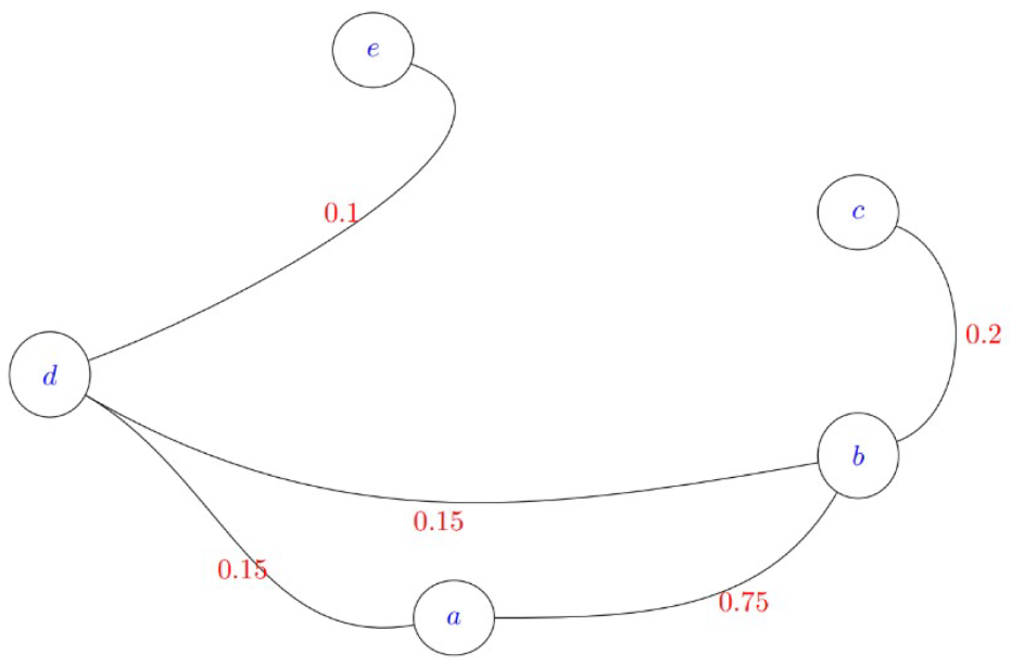
Example The picture below represents the weighted network of five nodes:

a, b, c, d

and e.

Let’s calculate the three topological properties introduced above for this graph example:

Degree The degree of this network is

\frac{(0.1 + 0.2 + 0.15 + 0.15 + 0.75) \times 2}{5 \times 4} = 0.135

Clustering Coefficient There is only one triangular connection in the network

a \to b \to d \to a

. As there are five different nodes, the number of all possible triangular connections is

C_{3}^{5} = 10

. Thus, the clustering coefficient is

1 / 10 = 0.1

Closeness To compute the closeness, let’s first look at the lengths of the shortest paths between each pair of nodes:

$s l_{a, b} = 0.3; s l_{a, c} = 0.5; s l_{a, d} = 0.15; s l_{a, e} = 0.25 .$
$s l_{b, c} = 0.2; s l_{b, d} = 0.15; s l_{b, e} = 0.25 .$
$s l_{c, d} = 0.35; s l_{c, e} = 0.45 .$
$s l_{d, e} = 0.1 .$

The closeness is

\frac{(0.3 + 0.5 + 0.15 + 0.25 + 0.2 + 0.15 + 0.25 + 0.35 + 0.45 + 0.1) \times 2}{5 \times 4 \times 4} = 0.0675

Next, we apply the methodologies and concepts developed and introduced above to study the stability of financial market, more preciously, the market is represented by some equity index, for instance S&P 500, Nasdaq, Dow 30, and so forth. The group of the (target) assets, which we are interested in, is the set of all the components of the selected index. We also have a carefully selected list of risk factors which covers almost all the major aspects of the real-world, thus, can be regarded a good proxy of it.

The group of target assets can vary quite differently due to the fact that the components of different equity indices can be very different. However, as the group of risk factors are selected as a complete proxy of the real-world, its components can be treated as universal and change in a very slow manner. We list some of the representatives of the risk factors below to illustrate how they look like.

Table 1. List of the Risk Factors for Network

Ticker	Name
U.S. Treasury	LUATTRUU INDEX
U.S. Corp	LUACTRUU INDEX
Global High Yield	LG30TRUU INDEX
Heating Oil	BCOMHO INDEX
Orange Juice	BCOMOJ INDEX
Euro (BGN)	EURUSD BGN Curncy
Japanese Yen (BGN)	USDJPY BGN Curncy
...	...

Now, we get back to discuss how to measure and predict the instability of the chosen equity index. At each time stamp t, we generate the PolyModel-Based correlation matrix for the component assets of the chosen index with respect to the universe of the selected risk factors, denoted as

M (t)

, then we can calculate the algebraic and topological quantities associated to

M (t)

. For every such quantity, we get a time series; to reduce the impact of noise, we can apply backward moving average or exponential decay to smooth the time series. These time series are the features. Sometimes, instead of these features themselves, we can consider their changes (like their first order derivatives) which also reflects the underlying network’s dynamics.

We are interested in the drawdown process of the selected index which represents the financial market. In particular, we will calculate the risk indicators based on PolyModel theory as described above, and analyze their relationships with the drawdown time series of DOW 30. More details are in the next section.

3. Experiment and Result

In this section, we will give an overview of the data sets used for the experiment, and then discuss the results, plots and further analysis.

3.1. Data Description

The equity index chosen to represent the financial market is DOW30, and the target assets are its components. We list some of the component tickers:

Table 2. List Some of the Component Tickers

SYMBOL	NAME
AXP	American Express Co
INTC	Intel Corp
KO	Coca-Cola Co
JPM	JPMorgan Chase & Co
DIS	Walt Disney Co
...	...

The universal pool of risk factors is the same as described in Section 5.3.

We generated the time series of 1st eigenvalue and degree of the PolyModel-Based correlation matrices of the components of DOW 30.

Then we calculated the drawdowns of DOW 30. Let’s first recall its definition in a formal way

Definition 7.

(Drawdown process definition 2.2 of [8]) Given a stochastic process

X_{t}

and a horizon T, the drawdown process is defined as

D_{t}^{(X)} = M_{t}^{(X)} - X_{t},

where

M_{t}^{(X)} = s u p_{u \in [0, t]} X_{u}

is the running maximum of X up to time t.

Drawdowns are a very good measure of the downside volatility, and measures how much one’s portfolio is down from the peak before it recovers back to the same level. When very large, it can also be treated as a sign of crisis.

3.2. Result and Analysis

In this part, we will check the relationships between dynamics of the algebraic or topological properties of the PolyModel-Based correlation matrix and the drawdown process of DOW 30.

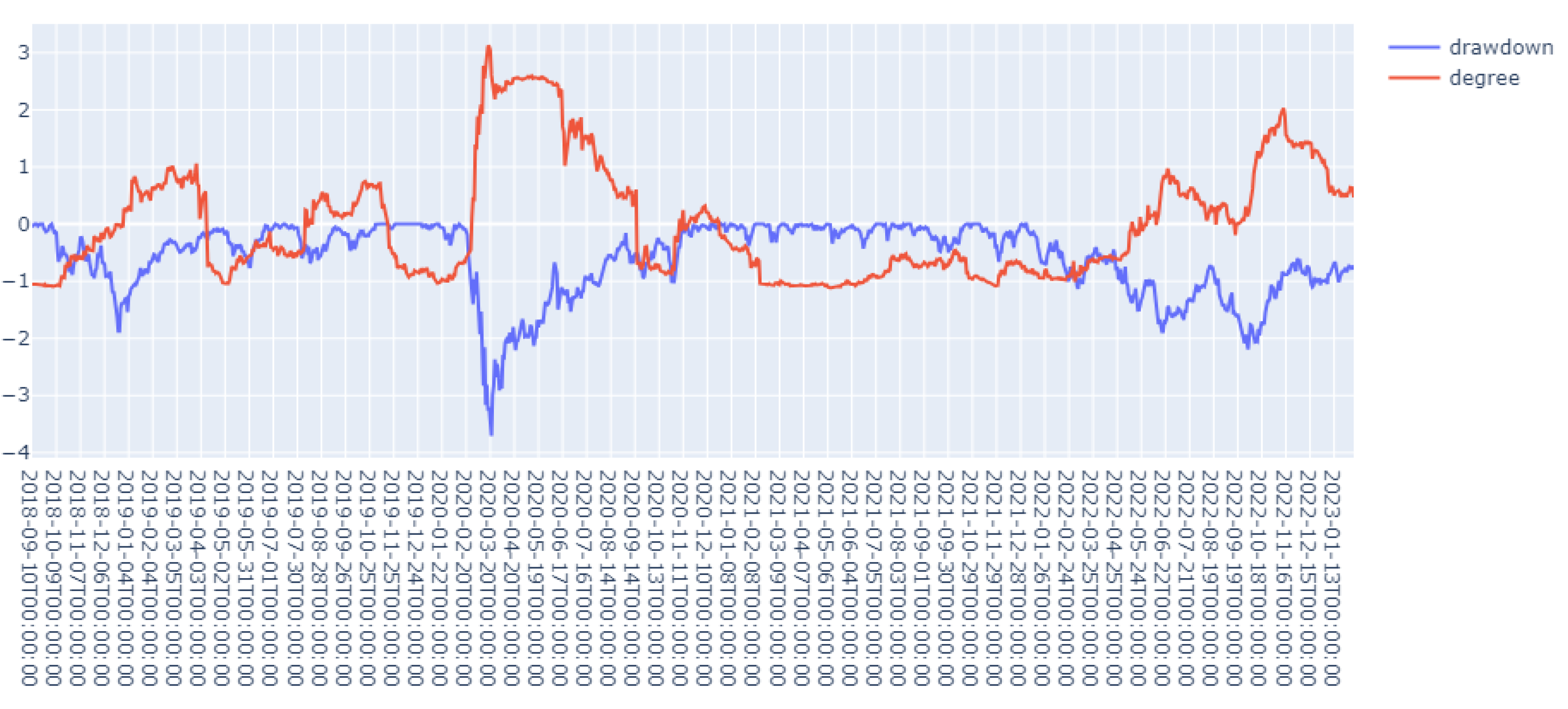
We calculated several such indicators, for instance, the first 3 eigenvalues, degrees, and the number of connected components. In general, these time series of indicators have quite similar behaviors, and we choose degree to illustrate the result. We compared the indicators at

t - k

against the drawdown process at t (k = 1 ∼ 5 business days), and we can see that a large value of peak of the indicators corresponds to the large drawdowns, and our indicator basically captured all the major drawdowns in advance (See the picture below as an example with

k = 3

). This again confirms that PolyModel theory is very good at capturing the downside market risks when the market goes down and there are only a few dominant risk factors.

Figure 1. Degree vs Drawdowns of DOW 30.

The above indicators can already capture and predict the relatively big drawdowns quite well. If we further would like our indicators more sensitive to the even small ones, we can further modify the indicators as follows.

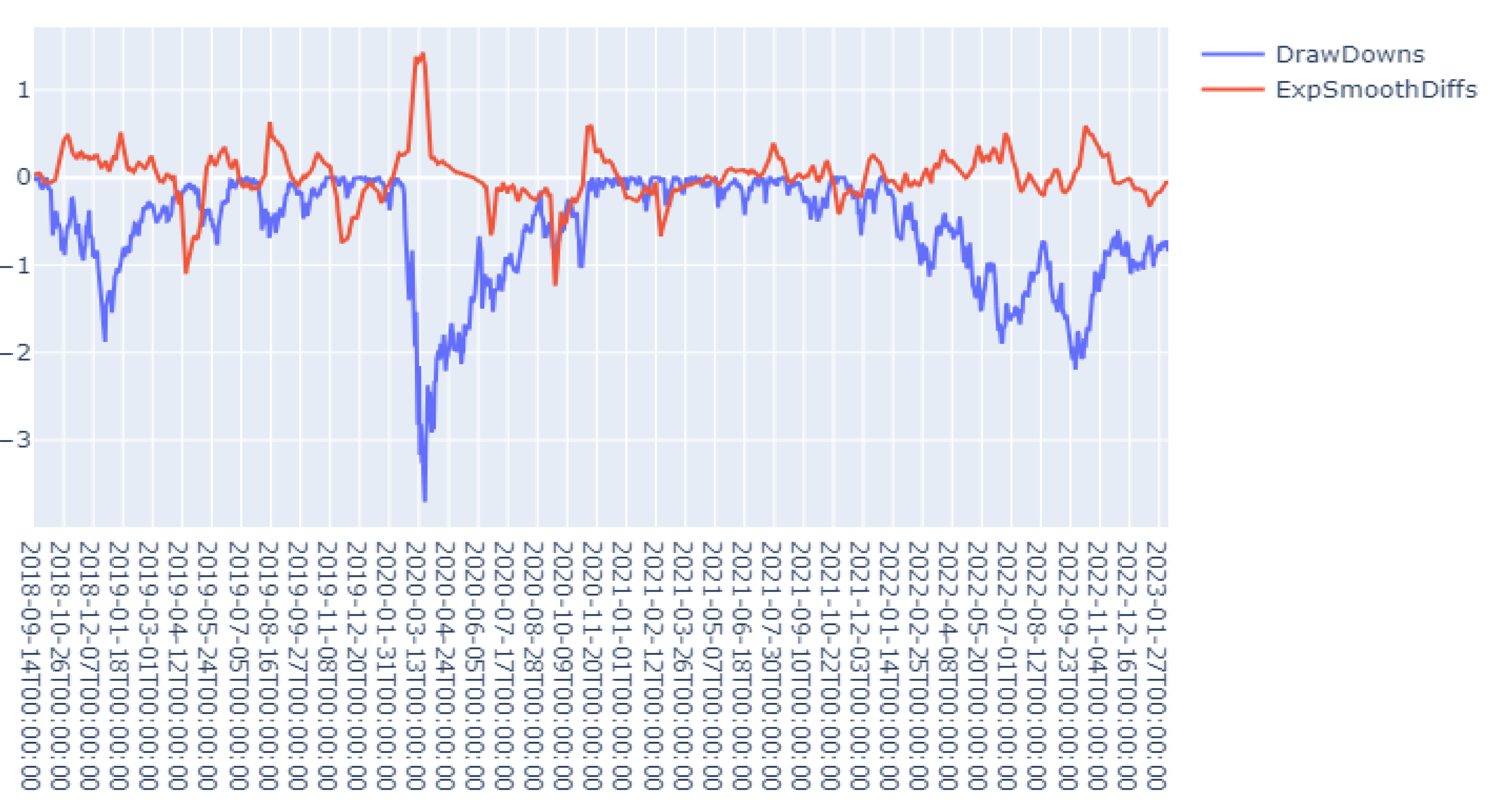
Suppose we choose indicator

I_{t}

from the above mentioned algebraic and topological properties. We set a back-ward time period

τ

and consider the new time series

d {(I)}_{t} : = I_{t} - I_{t - τ}

. This new indicator can help to capture how

I_{t}

evolves along with time which is usually more sensitive to the dynamical changes of the financial network. As such type of data is usually quite noisy, we also apply exponential decay to the new indicator time series

d {(I)}_{t}

in order to get its real trend. We applied this method to the 1st eigenvalue with

τ = 5

business days. Below is the picture to compare the new indicator at time

t - 3

with the drawdowns at time t:

Figure 2. Smoothed Difference of 1st Eigenvalue vs Drawdown.

4. Conclusions and Future Work

In this paper, we discussed how to construct a financial network, especially, we proposed the innovative network construction method based on PolyModel theory. This makes our proposed network not only captures the intrinsic correlations among different stocks but take the reactions of different stocks with respect to various outside factors as well. In the experiment, it shows that our methodology can capture or predict the major recession of the financial index.

In the present work, we are mainly working with statistical methods to analyze the constructed financial network. Along with the fast growth and development of modern machine learning techniques, more and more researchers have applied modern machine learning and deep learning methods in the financial field. Popular methods include long short term memory [9], transformer technique [6], etc. In the next work, we plan to apply these methods to make enhancement of the construction of the network, and to do better prediction of its structure change.

Another extremely active recent research area is large language model (LLM). There are many research on this topic, covering almost all its aspects. For our purpose and application, we hope to apply LLM to assist the construction, prediction and explanation of our financial network in an efficient and robust way. Fortunately, there have been researchers considering such questions: [10] for LLM’s performance and robustness, and [11] for LLM’s explanation power. We will apply these research result to enhance our study on the dynamic of financial network.

References

J.-P. Onnela, K. Kaski, and J. Kertsz. Clustering and information in correlation based financial networks. The European Physical Journal B - Condensed Matter, 38(2):353–362, Mar 2004. [CrossRef]
Romeil Sandhu, Tryphon Georgiou, and Allen Tannenbaum. Market fragility, systemic risk, and ricci curvature. arXiv preprint arXiv:1505.05182, 2015. arXiv:1505.05182, 2015.
Douglas Castilho, Tharsis T. P. Souza, Soong Moon Kang, João Gama, and André C. P. L. F. de Carvalho. Forecasting financial market structure from network features using machine learning. arXiv preprint arXiv: 2110.11751, 2021. arXiv:2110.11751, 2021.
Sameer Jain Xinfeng Zhou. Active Equity Management. Zhou, 2014. ISBN 9780692259283. URL https://books.google.com/books?id=CLEQnQAACAAJ.
Mauro Ursino, Giulia Ricci, and Elisa Magosso. Transfer entropy as a measure of brain connectivity: A critical analysis with the help of neural mass models. Frontiers in Computational Neuroscience, 14, 2020. ISSN 1662-5188. URL https://www.frontiersin.org/articles/10.3389/fncom.2020.00045. [CrossRef]
Siqiao Zhao, Zhikang Dong, Zeyu Cao, and Raphael Douady. Hedge fund portfolio construction using polymodel theory and itransformer, 2024. URL https://arxiv.org/abs/2408.03320.
Thomas Barrau and Raphael Douady. Artificial Intelligence for Financial Markets: The Polymodel Approach. Springer Nature, 2022.
Lisa R. Goldberg and Ola Mahmoud. Drawdown: From practice to theory and back again. arXiv preprint arXiv:1404.7493, 2016. arXiv:1404.7493, 2016.
Xiaojing Fan, Chunliang Tao, and Jianyu Zhao. Advanced stock price prediction with xlstm-based models: Improving long-term forecasting. Preprints, August 2024.
Xiaojing Fan and Chunliang Tao. Towards resilient and efficient llms: A comparative study of efficiency, performance, and adversarial robustness. arXiv preprint arXiv:2408.04585, 2024. arXiv:2408.04585.
Xinli Yu, Zheng Chen, Yuan Ling, Shujing Dong, Zongyi Liu, and Yanbin Lu. Temporal data meets llm – explainable financial time series forecasting, 2023. URL https://arxiv.org/abs/2306.11025.

Disclaimer/Publisher’s Note: The statements, opinions and data contained in all publications are solely those of the individual author(s) and contributor(s) and not of MDPI and/or the editor(s). MDPI and/or the editor(s) disclaim responsibility for any injury to people or property resulting from any ideas, methods, instructions or products referred to in the content.

© 2024 by the authors. Licensee MDPI, Basel, Switzerland. This article is an open access article distributed under the terms and conditions of the Creative Commons Attribution (CC BY) license (http://creativecommons.org/licenses/by/4.0/).

Copyright: This open access article is published under a Creative Commons CC BY 4.0 license, which permit the free download, distribution, and reuse, provided that the author and preprint are cited in any reuse.

MDPI Initiatives

Important Links

Choose an area of interest and we will send you notifications of new preprints at your preferred frequency.

Disclaimer

Financial Network Analysis Using Polymodel Theory

Abstract

1. Introduction

2. Methodology

2.1. Notations

2.2. PolyModel-Based Time Series Relationship

2.3. Financial Network Construction and Analysis

3. Experiment and Result

3.1. Data Description

3.2. Result and Analysis

4. Conclusions and Future Work

References

MDPI Initiatives

Important Links

Subscribe