1. Introduction
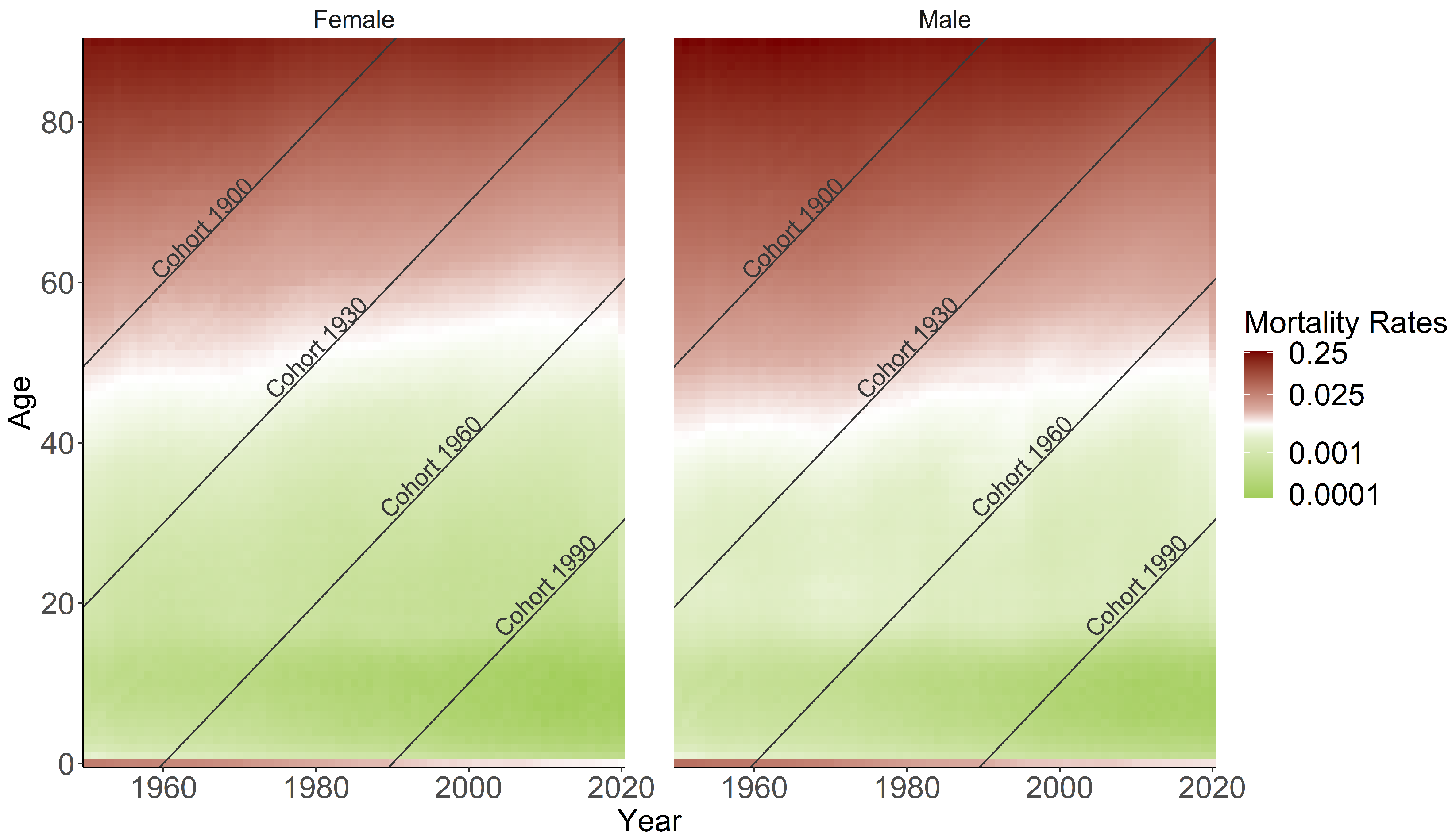
In recent decades, life expectancy in the developed world has shown a substantial increase, exemplified by a notable 56.7% reduction in the mortality rate of 80-year-old men in the USA from 1933 to 2019. This trend, reflecting societal advancements and improved healthcare systems, underscores the importance of accurately predicting mortality trends for informed decision-making by policymakers, pension schemes, insurers, and social security systems. The emergence of the COVID-19 pandemic has further underscored the need to understand its impact on mortality trends over the short to mid-term. Our study focuses on assessing the impact of COVID-19 on mortality trends, aiming to enhance existing mortality models while maintaining explainability.
The literature presents a diverse range of approaches to mortality modeling, from traditional stochastic models like those discussed by [
31], to modern methods such as the use of machine learning (ML) techniques. Recent studies have shown that methods like pure Gradient Boosting or Random Forests perform exceptionally well [
34], while others have explored hierarchical approaches with ML building upon simpler LC models [
30]. Furthermore, recent advancements include the application of neural networks to enhance mortality models, such as the Common-Age-Effect Model proposed by [
32], and the extension of LC models for multiple populations demonstrated by [
33]. Generalized Additive Models (GAMs), a well-established model class was first introduced by [
39], and has been applied in mortality context, [
38] describes a Bayesian APC model with an autoregressive prior on the age, period and cohort terms, also [
28] proposed the use of a bivariate spline function within a GAM to effectively capture two-dimensional cohort information. A similar model was applied by [
37] for projecting cancer incidence and mortality in Finland, [
36] for mortality in the UK and by [
35] for projecting breast cancer mortality in Spain. However, none of them is modeling and extrapolating GAM in APC framework with a tensor product in a multi-populational fashion. The literature on accounting for COVID in mortality projections is also growing, such as [
48] that uses stochastic Li and Lee model, [
50] that proposes parsimonious decomposition of the mortality surface on a polynomial basis with regularization and cross-validation, [
32] that quantifies the impact of the 2020 mortality shock by calibrating the Lee–Carter model. However, none of the aforementioned studies employ GAM in APC and evaluate scenarios post-pandemic.
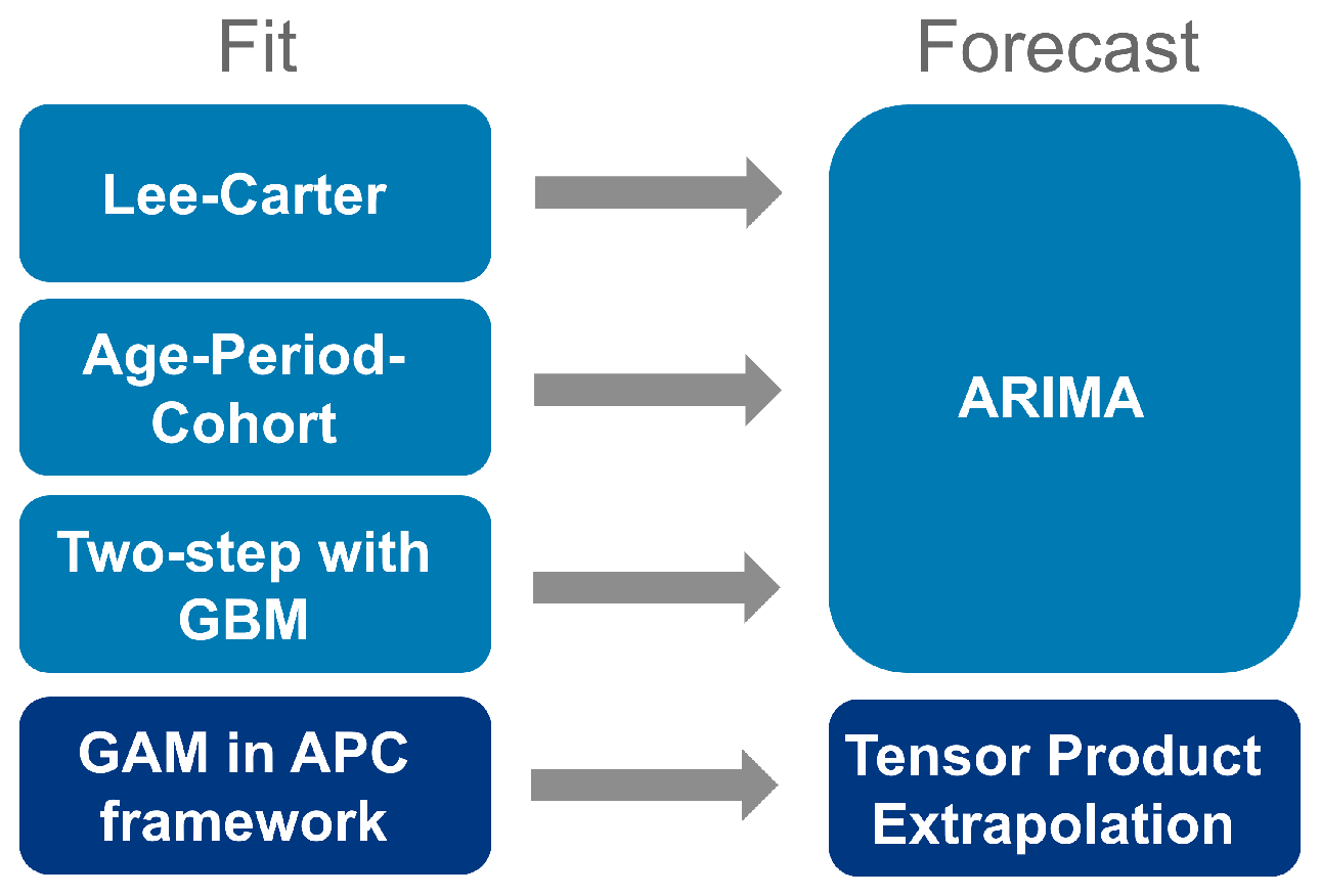
To compare with traditional stochastic mortality models LC [
31] and Age-Period-Cohort (APC) [
17], alongside contemporary ML methodology proposed by [
30], this study introduces a cross-country GAM within an APC framework, utilizing a smoothed second-order spline with penalty points. To our knowledge, this research is the first to integrate the GAM method into the APC framework in a multi-population context and employ it to extrapolate the impact of COVID-19 on future mortality trends. We examine Germany, Finland, the Netherlands, Italy (representing Europe), and the United States (representing North America) using data from the Human Mortality Database [
56]. We employ a cross-country approach, enabling the model to learn from multiple countries concurrently, thereby capturing both universal trends and country-specific variations in mortality patterns.
Our research makes three key contributions. First, we compare the predictive performance of four models, including traditional single-population and contemporary multi-populational models, for modeling and projecting future mortality rates for five countries. We find that the most promising approach is based on a GAM, where cohorts are represented as an interaction between age and period. This framework, adaptable for both aggregated and individual survival data, introduces a state-of-the-art method for the field of multi-populational cross-country mortality research. Secondly, we introduce partial APC plots as a novel graphical tool in mortality research, enabling the analysis of specific APC structures. This tool aids in communicating complex temporal patterns and highlights gender-specific and cross-country differences. Finally, we provide fresh insights into the factors driving the impact of the COVID-19 pandemic on mortality. Through analyzing age, period, and cohort associations in a multi-population context using a GAM within an APC framework, we extrapolate mortality rates into the future. Four scenarios, representing varying degrees of pandemic impact, are evaluated against observed mortality data post-pandemic to identify the most accurate scenario.
The practical implications of our findings are considerable. Our research demonstrates the efficacy of the GAM within the APC framework and its capacity to extrapolate mortality forecasts, accounting for the impact of the COVID-19 pandemic. This offers invaluable insights for policymakers and stakeholders, providing guidance in navigating the uncertainties brought about by the pandemic, with a particular emphasis on matters pertaining to life insurance and pension funds.
Our study follows a structured approach, beginning with an overview of the database and methodology. We then compare the predictive performance of benchmark methods across countries, offering insights into optimal trend forecasting techniques. Additionally, we conduct scenario analyses to evaluate the impact of COVID-19 on mortality trends. Finally, we conclude by summarizing our key findings and implications.
3. Results
This section begins with an evaluation of predictive performance, both in-sample and out-of-sample, for all four models.
Table 1 gives an overview of the different training and test sets used in the analysis. It should be noted that for the purposes of benchmarking, years up to and including 2019 are used, on the assumption that they are not affected by the impact of the COVID-19 pandemic. This approach eliminates any year-specific artefacts that might otherwise affect the assessment of the predictive performance of the models themselves. The single-populational models LC, APC, and GBM (based on LC in the first step) are limited to using data from Germany from 1990 onwards due to data inconsistencies before reunification. In order to maintain comparability across the tensor-product spanned by years and ages, it is necessary to ensure that the multi-population GAM is coherent. This is because GAM requires a joint coverage of years ‒ a prerequisite for coherent modelling. As a result, available years for all countries will be restricted to 1990-2015 to ensure sufficient training for capturing current effects on mortality rates and projecting them into the future for 2016-2019.
Focusing on in-sample RMSE for single-populational LC, APC, multi-populational GBM, and GAM models, we fit the training periods range from 1950 to 2010 for Finland, Italy, the Netherlands, and the US, and from 1990 to 2010 for Germany. GAM models are fitted from 1990 to 2015 for all countries. In-sample error is calculated within the same range as the model training period and reveals that the two-step approach with GBM and GAM in the APC framework exhibit superior performance over traditional stochastic mortality models LC and APC. There is no clear preference between GBM and GAM, both achieving strong reductions in RMSE compared to LC and APC for in-sample predictions.
Table A1 in
Appendix C provides a comprehensive analysis of the goodness-of-fit.
Table 2 presents the out-of-sample results for different models, indicating the forecasting quality across countries and genders. Out-of-sample RMSE is calculated based on forecast periods ranging from 2011 to 2019 for LC, APC, and GBM models, while GAM forecasts span from 2016 to 2019 for all countries.
Although different forecast methods are applied and different years are tested, RMSE serves as a comparable estimator for mean error. While GBM shows improved fit and forecast performance, GAM exhibits stronger improvement in forecast accuracy, especially for short-term forecasts within a few years. The GAM-based APC model achieves notable reductions not only in fit but also in forecast errors compared to the classical APC model, implying improved accuracy of mortality rate predictions. The choice of GAM for further analysis is justified based on its superior forecast performance.
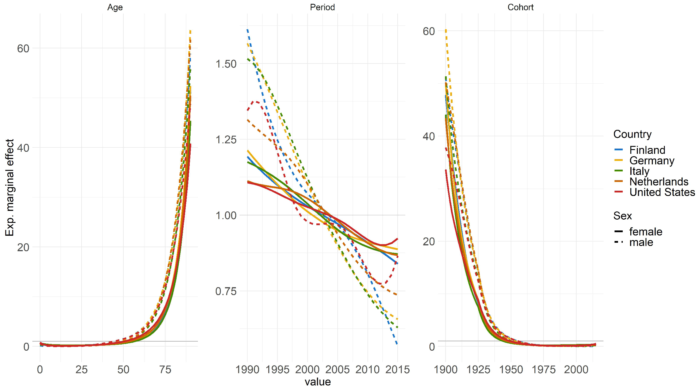
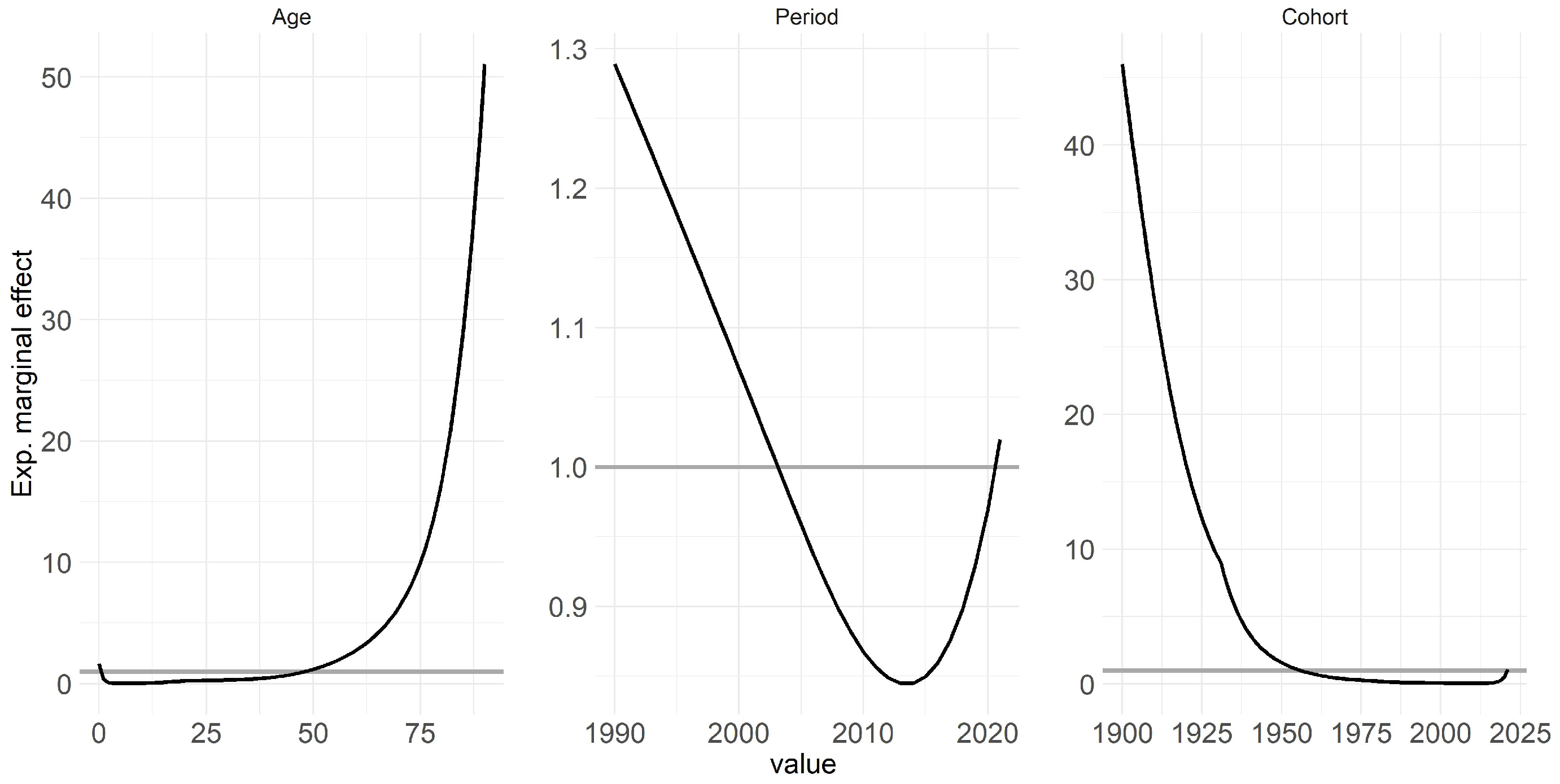
One key highlight of the GAM in APC framework is its multi-populational nature, enabling the interpretation of exponential marginal effects, with age, period, and cohort being the components analyzed further.
Figure 3 displays the effects of the model based on these components: Both age and cohort effects conform to expectations, thus higher ages correspond to higher mortality rates, while cohort effects reflect variations stemming from individuals’ unique experiences based on their birth year [
2,
3,
4]. Conversely, similar reverse effects are observable for age and cohort.
The period effect, which indicates the improvement of mortality over time and is influenced by external factors affecting all age groups equally at a given point in time, exhibits a notable increase leading up to 2020 [
1,
14]. However, the period effect notably spikes, particularly approaching 2020, signifying a strong influence of this year on mortality rates. Specifically, the strides made in improving mortality rates over preceding years or even decades appear to have been offset by the effect of COVID-19, resulting in a regression to levels observed around 2003.
Appendix C contains this figure stratified by countries and genders for more detailed interpretation.
Following the benchmarking of the four models, we delve into an analysis of the effects of each temporal component on mortality rates throughout the considered time period. Finally, based on GAM in APC frameworkwe assess the trend forecast into the future considering COVID-19 impact.
Even though the impact of COVID-19 is, fortunately, diminishing in the present time, its impact on historical (and future) data and the persisting uncertainties in the future cannot be overlooked. These factors necessitate continued attention for many years to come. It is important to note that the idea and methodology employed in this study extend beyond COVID-19 and encompass other events, especially those occurring at the edge of time series, which can present challenges for standard breakpoint analyses.
The scenarios depicted herein must be viewed in light of a meticulous plausibility assessment and the underlying assumptions. To validate the scenario-based findings, we engaged with epidemiological experts. This collaboration is paramount for ensuring the reliability and robustness of the analysis, especially given the complexities inherent in such events. Comparing our framework with expert opinions in the literature, as done by [
9], reveals a high level of agreement.
Four different scenarios are defined to provide insights into the potential future trajectories of mortality, taking into account various assumptions about the impact of COVID-19.
Table 3 summarizes the different training and test periods used in the scenario analysis, now considering also years after 2019.
Scenario 1: In this scenario, the assumption is made that COVID-19 will disappear in the future. The model is trained using data up to 2019 only, excluding the years 2020 and 2021. The predictions are then made for the years 2020-2025, assuming no long-term effects of COVID-19 on mortality. This approach treats COVID-19 as a special event that does not have any influence on mortality in the upcoming years. The model focuses on the underlying mortality trend without considering the impact of COVID-19 and thus without the covid-indicator.
Scenario 2: In Scenario 2, the expectation is that the full COVID-effect will persist in the future. The model is trained on mortality data up to and including 2021, encompassing years impacted by COVID-19. The indicator variable is incorporated, set to 0 for years before 2019 and 1 for 2020 and 2021. Predictions are then made for subsequent years, assuming remains set to 1 to indicate the ongoing presence of COVID-19. This scenario assumes that the COVID-related situation will continue similarly as it did until 2021, and that it will have a consistent effect on mortality over the coming years.
Scenario 3: In this scenario, the assumption is made that the COVID-effect will flatten over time. Similar to Scenario 2, the model is trained using mortality data up to and including 2021. However, in this case, the COVID-19 effect is assumed to decrease exponentially over time. The predictions take into account the diminishing impact of COVID-19 in the future, reflecting the belief that the effect of COVID-19 on health and mortality will slowly flatten out and eventually disappear after a few years. Therefore, the indicator takes exponentially decreasing values between 1 and 0 for each year.
Scenario 4: In Scenario 4, the focus is on adjusting for excess mortality associated with COVID-19. The years 2020 and 2021 are treated as outliers, but the excess mortality is explicitly considered. The model calculates the difference between the expected death counts and the actual mortality counts for these two years to account for the excess mortality. It is assumed that the excess mortality will not average out over the coming years and must be explicitly accounted for. The baseline mortality, representing the mortality trend without the influence of COVID-19, remains unchanged. This scenario allows for separate consideration of the excess mortality caused by COVID-19 while keeping the baseline mortality unchanged.
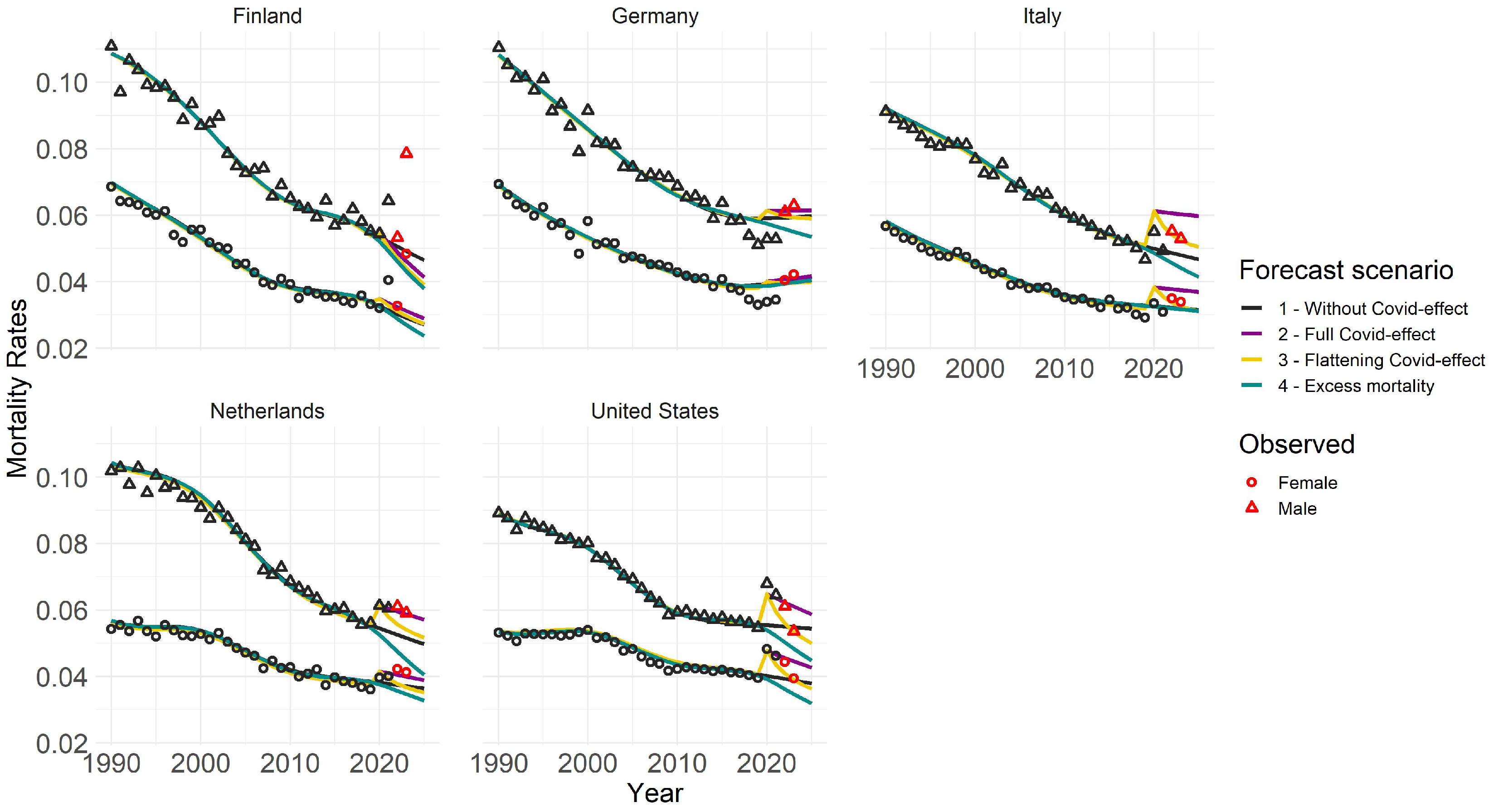
Figure 4 presents outcomes for four scenarios across various countries and genders, focusing on 80-year-olds. We chose age 80 for illustration, but the overall structure is similar for other ages, albeit with less intense COVID-19 effects for younger age groups. Notable high value outliers for Italy, the US, and the Netherlands in 2020 and 2021 indicate a pronounced impact of COVID-19. Different trend forecasts capture varying effects of COVID-19 on mortality rates. Scenario 1 represents a milder assumption, while Scenario 2 depicts a more severe projection. Future forecasts vary by country and age group, influenced by past behaviors and responses to the pandemic. Trend forecasts in different scenarios generally align with plausibility. Excluding 2020 and 2021 in Scenario 1 results in lower mortality rates, while adjusting for excess mortality in Scenario 4 leads to even lower rates, considering the population shift due to previous deaths. Scenario 2 with full COVID effect shows the highest mortality trend, particularly evident for older age groups. However, younger populations appear less affected. Scenario 3 starts similar to the Scenario 2 but gradually decreases over time. Different countries show distinct trends, likely influenced by COVID’s demographic and political impact. The Netherlands’ observed rates in years 2022 and 2023 align with the Scenario 2, whereas Italy and the US show patterns more consistent with the flattening effect. German scenarios show less differentiation, aligning closely with observations, while Finland’s forecast suggests lower mortality rates than observed.
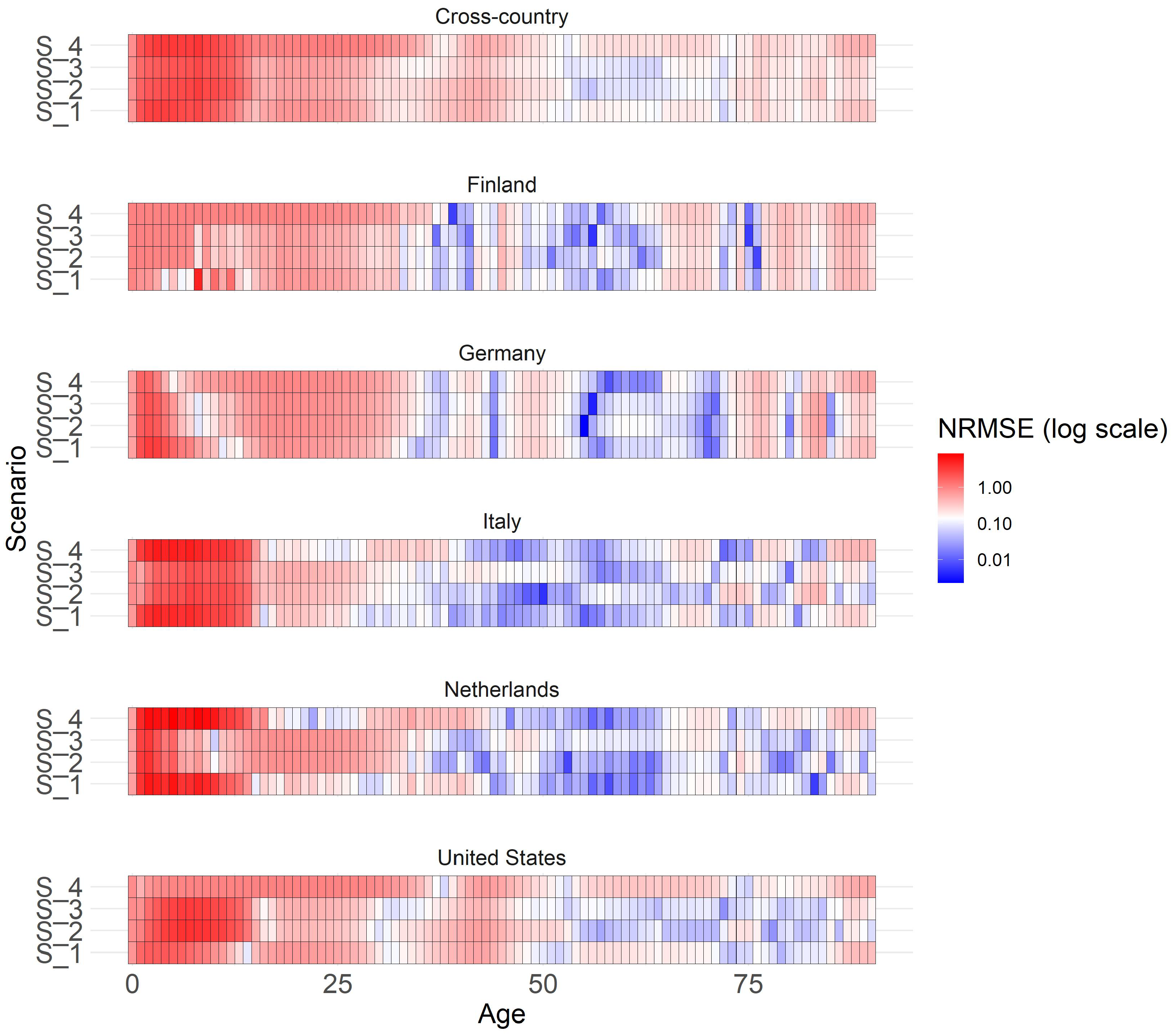
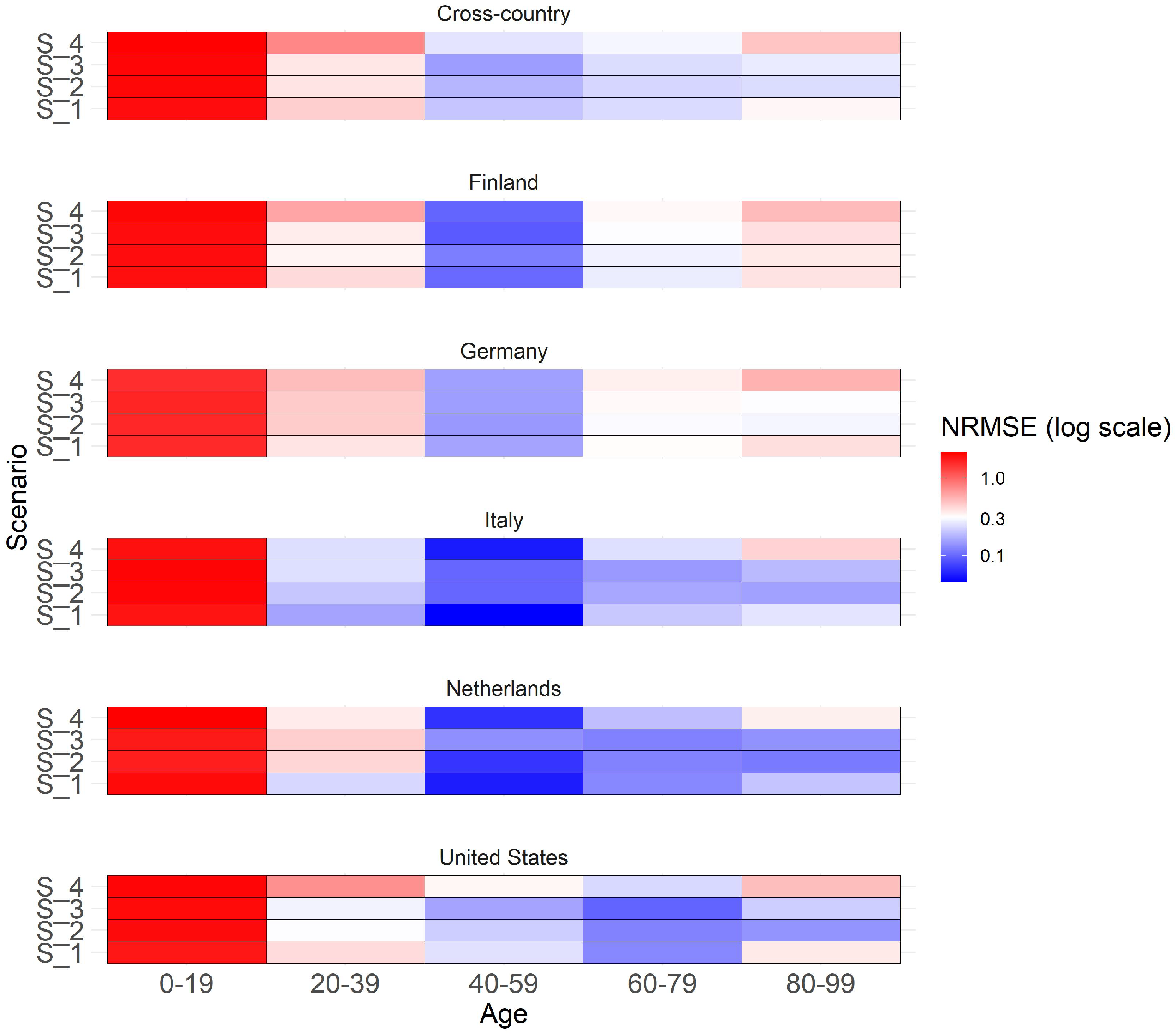
The heatmap (
Figure 5) illustrates both a cross-country and country-specific perspective on the y-axis, while age groups are delineated on the x-axis. Colors within the heatmap indicate the normalized RMSE (NRMSE) values for the years 2022 and 2023, when compared with the observed mortality rates from STMF and processed in accordance with
Appendix A.
NRMSE is calculated by dividing RMSE by the mean of observed mortality rates in a specific category with values ranging usually from 0 to 1. A value of 0 means perfect predictions, while 1 suggests predictions are as accurate as predicting the mean. Values above 1 often suggest that the model’s performance may not be optimal. We prioritize the analysis on males since previous findings suggest a more pronounced emphasis on the COVID effect for this gender, although the overall patterns for females exhibit similarity. For males in 20-year age brackets, the graph shows a generally good overall forecast accuracy, especially for ages over 20, as colors tend towards blue for middle and older ages, indicating smaller NRMSE values, closer to 0, suggesting better forecast accuracy. No clear scenario preference is evident in the cross-country view across all age groups. In general, Scenario 3 (flattening COVID effect) tends to perform well for middle-aged individuals and in addition also Scenario 4 (COVID full effect) for older ages. Substantial variations in scenario performance are observed across different countries and age groups. For younger age groups, Scenario 1 (no COVID effect) performs best in Italy and the Netherlands, where substantial COVID impact was observed. Middle-aged groups demonstrate similarly high performance across all scenarios. Older age groups show stronger scenario differences with a clear preference for Scenarios 2 and 3, indicating better fit. Scenarios do not perform well for those under 19, possibly due to the unique characteristics and weak impact of COVID in this age group.
Appendix C contains the same graph with individual ages instead of grouped age buckets for more detailed overview.
4. Conclusion
To summarize, this research work focused on addressing the challenge of capturing the mortalit-related extreme event at the edge of a time series, in particular, COVID-19 effect in future mortality forecasting.
The study applies the GAM in the APC framework with penalized smoothing second-order splines to forecast future mortality trends in a cross-country fashion. To compare the predictive performance against traditional stochastic mortality models and more contemporary approaches with GBM, the research considers data of Germany, Finland, the Netherlands, Italy, and the United States retrieved from HMD, supplemented with prepared data from STMF. The study defines four future scenarios to facilitate trend forecasting and provide insights into the potential impact of COVID-19 on mortality rates, spanning from mild to severe. To ensure a rigorous assessment, these scenarios and their underlying assumptions were thoroughly evaluated and discussed in collaboration with epidemiological experts. This approach including the content of scenarios aligns with existing literature and enhances the credibility of the forecast analysis [
9].
Overall, this work contributes to the existing literature by introducing traditional, enhanced and novel models, comparing different approaches, and providing insights into the future development of mortality rates, considering the impact of COVID-19 in a cross-country context. The specific contribution of the GAM approach with the APC framework in this research lies in its novel application for mortality trend forecasting, particularly incorporating the impact of COVID-19 in multi-populational cross-country fashion.
Despite the waning impact of COVID-19 at present, it is crucial to recognize the enduring importance of historical data and the persisting uncertainties that lie ahead. These factors emphasize the need for ongoing attention in the years to come. It is important to acknowledge that the concept and methodology utilized in this study extend beyond COVID-19, encompassing other events that occur at the fringes of time series data. Looking towards future research directions, the GAM with APC framework has a promising potential for expanding the feature set by the inclusion of socioeconomic status, income, education as additional factors, allowing for a more comprehensive understanding of mortality trends.
Appendix A. Data Preparation
This section discusses the methodology employed to enrich existing mortality data obtained from [
57], focusing on the number of deaths and population size for recent years absent in the [
56] dataset. The primary challenge addressed is the aggregation of data into rough age categories, while the study requires a metric age scale.
The methodology involves several steps. Firstly, weekly population sizes are derived from the mortality dataset, followed by extrapolation to annual levels. Using mortality rates and death counts, the weekly population size can be calculated. This weekly data is then aggregated to annual figures. Similarly, weekly death counts are summed to obtain annual totals. To construct annual death counts and populations for individual ages for the aforementioned years, specific procedures were applied, as described below. The methodology ensures that the derived data aligns with observed mortality patterns within each age group.
Once the weekly population is extrapolated to the annual level by multiplying with a factor of 52, the approach leverages cohort-wise population patterns from previous years (2015-2019) and assumes a similar age distribution for 2020-2023. The initial population course i.e. for 2020 is created by shifting the population size pattern of 2019 one year forward. This shift leads to an initial gap at age 0 in 2020, which is linearly extrapolated based on data from 2018 and 2019. The resulting population values are adjusted to match observed data within age groups.
A three-stage approach is employed to distribute death counts from grouped to metric age scale on an annual basis. Firstly, averaged weights for each age in each age bucket are computed based on data from the previous five years (2015-2019): . Secondly, these weights are applied to the averaged death counts in each age group to correct for deviations from the mean: . Finally, the corrected death counts are adjusted to ensure equal counts in both grouped and metric versions within each age group:
The resulting mortality rates are computed by dividing death counts by population size for each individual age and subpopulation. This enriched mortality data is used to impute the [
56] dataset for the years 2020-2023. The same procedure is applied across all subpopulations and missing years.
Appendix B. Details on Gradient Boosting Machine
Gradient Boosting is another form of an ensemble learner that is based on the weighted combination of weak predictive learners such as Decision Trees, usually outperforming Random Forest [
23]. The model is built stepwise and optimized by a differentiable loss function, minimizing the in-sample loss [
23]. It builds the model stepwise, like other boosting methods, and generalizes them by allowing optimization of any differentiable loss function. Whereas in bagging multiple samples of the original training dataset are used to fit a separate decision tree to each one independent of the others and to combine all trees into a single predictive model, boosting grows the trees sequentially, meaning the information gained from the previous trees is used to grow the current one. This helps to overcome the major issue of training a single large Decision Tree by possibly resulting in an overfitting problem. The gradient boosting algorithm instead learns by constructing a new model based on the previous one and adding the
base learner
:
The model is improved in such a way that the current residual will be used as an outcome to fit a new Decision Tree and to add this into the originally fitted function with the notion to update the residuals. So, the gradient boosting algorithm fits the new predictor to the residual errors made by the previous predictor. The shrinkage parameter
helps to run the process even slower allowing for more trees and more detailed enhancement of the residuals. All parameters of the Decision Trees undergo optimization through the training of Poisson boosted trees, with the objective of minimizing the negative log-likelihood associated with the Poisson distribution, serving as the designated loss function. Overall in contrary to the bagging methodology, each tree depends on the previous ones [
7]. Even though the gradient boosting keeps on minimizing the errors, this can cause overfitting in case of a lot of noise in the data and is computationally time and memory expensive, especially because trees are built sequentially (not in parallel as the Random Forest do). Due to the high flexibility, the gradient boosting algorithm also tends to be harder to tune than Random Forest [
23]. In this study, we specifically utilized LightGBM [
59] employing Microsoft’s library for implementing these models, which have demonstrated high accuracy in various scenarios [
58].
Appendix C. Additional Results
The analysis in
Table A1 highlights the superior in-sample predictive performance of the two-step GBM and GAM models within the APC framework over traditional LC and APC models, with no clear preference between GBM and GAM, across various training periods for different countries.
Table A1.
In-sample RMSE comparison for LC, APC, GBM, and GAM models. LC, APC, and GBM are fitted from 1950 to 2010 (Finland, Italy, Netherlands, US) and 1990 to 2010 (Germany). GAM is fitted from 1990 to 2015 for all countries.
Table A1.
In-sample RMSE comparison for LC, APC, GBM, and GAM models. LC, APC, and GBM are fitted from 1950 to 2010 (Finland, Italy, Netherlands, US) and 1990 to 2010 (Germany). GAM is fitted from 1990 to 2015 for all countries.
| Country |
Female |
|
Male |
| |
|
LC |
|
APC |
|
GBM |
|
GAM |
|
LC |
|
APC |
|
GBM |
|
GAM |
| FIN |
|
0.0045 |
|
0.0015 |
|
0.0035 |
|
0.0011 |
|
0.0072 |
|
0.0027 |
|
0.0066 |
|
0.0013 |
| DE |
|
0.0015 |
|
0.0022 |
|
0.0004 |
|
0.001 |
|
0.0021 |
|
0.0021 |
|
0.0007 |
|
0.001 |
| ITA |
|
0.0025 |
|
0.0021 |
|
0.001 |
|
0.001 |
|
0.0012 |
|
0.0025 |
|
0.0008 |
|
0.001 |
| NLD |
|
0.0019 |
|
0.0032 |
|
0.0014 |
|
0.001 |
|
0.0017 |
|
0.0015 |
|
0.0014 |
|
0.001 |
| US |
|
0.0014 |
|
0.0033 |
|
0.0005 |
|
0.0013 |
|
0.0017 |
|
0.0028 |
|
0.0004 |
|
0.0011 |
Figure A1.
Estimated marginal effects of age, period, and cohort on mortality rates, differentiated by countries and genders. The horizontal lines represent the level of no effect. The GAM model was fitted for the years 1990-2015 and ages 0-90.
Figure A1.
Estimated marginal effects of age, period, and cohort on mortality rates, differentiated by countries and genders. The horizontal lines represent the level of no effect. The GAM model was fitted for the years 1990-2015 and ages 0-90.
GAM enables the interpretation of exponential marginal effects, with age, period, and cohort being the components analyzed and differentiated by countries and gender. Notably, while the descending trend in period effect for women is relatively consistent and shallow across all countries, men exhibit a much steeper decline, indicating a stronger improvement in mortality rates over the years. There are noticeable increases in mortality rates for Italy and the US in recent years, particularly for US males, which may be associated with factors such as the opioid crisis.
Figure A2.
Heatmap showing the normalized RMSE of scenarios for extrapolated years 2022 and 2023 for males across different countries and individual ages.
Figure A2.
Heatmap showing the normalized RMSE of scenarios for extrapolated years 2022 and 2023 for males across different countries and individual ages.
The heatmap depicted in
Figure A2 offers a detailed examination on an individual age basis for assessing the scenario analysis across the years 2022 and 2023.
